A Tutorial on Diffusion Models (Part 1)
DDPM with Tensorflow2 implementation
Resources
- The Jupyter notebooks associated with this tutorial can be found here
- The slide can be found here: (Dinh’s revision).
- The lecture about Generative Models which includes VAE, GAN and Diffusion Models that I taught at VietAI is available here.
DDPM
When talking about diffusion models, we usually refer to three notable works including Sohl-Dickstein et al., 2015
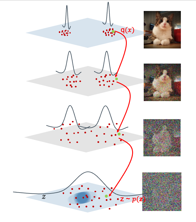
The general diffusion framework includes two processes: the forward diffusion process in which a random noise is added to an input image to destruct the image, and the backward (reverse) diffusion process in which the image is denoised by removing the noise added in the forward diffusion process to reconstruct the original image.
Forward Diffusion Process

In the DDPM model, the forward diffusion process is formulated as Markov chain with T steps such that at each time step \(t\), the image \(x_t\) is distributed according to a Gaussian distribution \(x_t \sim q(x_t \mid x_{t-1}) = \mathcal{N}(x_t \mid \mu_t, \sigma_t^2)\) with mean \(\mu_t=\sqrt{1-\beta_t} x_{t-1}\) and variance \(\sigma_t^2 = \beta_t I\), where \(0< \beta_t < 1\) is the diffusion coefficient at time step \(t\).
Intuitively, in the input space, data points are usually not uniformly distributed in the entire space, but they are usually concentrated in some regions with high density (as illustrated in the following figure). Therefore, the diffusion process can be seen as a process to spread out the data points in the input space, which is similar as the process of diffusion in physics. Analogy speaking, we can imagine that the entire possible input space is a room filled with air, and the data points are some heat sources in the room. The air molecules will move randomly (Brownian motion) in all directions and collide with neighboring molecules. As a result, the heat will be spread out from the high density regions to the low density regions. This process will continue until the temperature is uniform in the room (reaching the equilibrium state). Back to the forward diffusion process in DDPM, at the time step \(t\), the image \(x_{t-1}\) is added with some noise so that \(x_t \sim \mathcal{N}(x_t \mid \mu_t, \sigma_t^2)\) with the variance is a little bit larger than previous step (lower density). This process will continue until the image \(x_T\) is completely destroyed (reaching the equilibrium state).

How to sample \(x_t\). While it is possible to form a Gaussian distribution \(q(x_t \mid x_{t-1})\) and sample \(x_t\) from this distribution, it is computationally expensive. Scaling to the Markov chain with \(T\) steps, this is obviously not a nice solution. Instead, by using reparameterization trick, the authors proposed a more efficient way to sample \(x_t\) as follows:
\[x_t = \sqrt{1-\beta_t} x_{t-1} + \sqrt{\beta_t} \epsilon_t\]where \(\epsilon_t \sim \mathcal{N}(0, I)\) is a standard Gaussian noise. This simple trick not only allows us to sample \(x_t\) efficiently from \(q(x_t \mid x_{t-1})\), but magically also allows us to jump to any arbitrary time step \(t\) and sample \(x_t\) from that. Details of this trick can be found in the original paper. Basically, \(x_t \sim q(x_t \mid x_0) = \mathcal{N}(x_t; \sqrt{\bar{\alpha}_t} x_0, (1-\bar{\alpha}_t)I)\) where \(\bar{\alpha}_t = \prod_{i=1}^{t} (1-\beta_i)\).
Let’s define \(\alpha_t = 1 - \beta_t\), then \(\bar{\alpha}_t = \prod_{i=1}^{t} \alpha_i\). With \(\epsilon_t \sim \mathcal{N}(0, I) \; \forall t \in [1, 2, ..., T]\), we have:
\[x_t = \sqrt{\alpha_t} x_{t-1} + \sqrt{1-\alpha_t} \epsilon_t\] \[x_{t-1} = \sqrt{\alpha_{t-1}} x_{t-2} + \sqrt{1-\alpha_{t-1}} \epsilon_{t-1}\] \[...\] \[x_1 = \sqrt{\alpha_1} x_0 + \sqrt{1-\alpha_1} \epsilon_1\]Replacing \(x_{t-1}\) in the first equation with the second equation, we have:
\[x_t = \sqrt{\alpha_t} (\sqrt{\alpha_{t-1}} x_{t-2} + \sqrt{1-\alpha_{t-1}} \epsilon_{t-1}) + \sqrt{1-\alpha_t} \epsilon_t\] \[x_t = \sqrt{\alpha_t \alpha_{t-1}} x_{t-2} + \sqrt{\alpha_t (1-\alpha_{t-1})} \epsilon_{t-1} + \sqrt{1-\alpha_t} \epsilon_t\]As mentioned very briefly in the paper ![]() ). Applying the same reparemeterization trick, we can have:
). Applying the same reparemeterization trick, we can have:
where \(\epsilon \sim \mathcal{N}(0, I)\).
Finally, we have:
\[x_t = \sqrt{\bar{\alpha}_t} x_0 + \sqrt{1-\bar{\alpha}_t} \epsilon\]where \(\bar{\alpha}_t = \prod_{i=1}^{t} \alpha_i\). This allows us to jump to any arbitrary time step \(t\) and sample \(x_t\) from that.
Properties of the forward diffusion process:
- At any arbitrary time step \(t\), we have \(q(x_t \mid x_0) = \mathcal{N}(x_t; \sqrt{\bar{\alpha}_t} x_0, (1-\bar{\alpha}_t)I)\).
- \(\sqrt{\bar{\alpha}_t}\) is a bit smaller than \(\sqrt{\bar{\alpha}_{t-1}}\), while \((1-\bar{\alpha}_t)\) is a bit larger than \((1-\bar{\alpha}_{t-1})\). Which is similar as the process of diffusion in physics when the temperature is spread out from the high density regions \(\mathcal{N}(x_{t-1}; \sqrt{\bar{\alpha}_{t-1}} x_0, (1-\bar{\alpha}_{t-1})I)\) to the low density regions \(\mathcal{N}(x_t; \sqrt{\bar{\alpha}_t} x_0, (1-\bar{\alpha}_t)I)\).
- If T is large enough, \(\bar{\alpha}_t \approx 0\), therefore, \(q(x_T \mid x_0) \approx \mathcal{N}(x_t; 0, I)\) which is the equilibrium state of the diffusion process.
Backward Diffusion Process

In the backward process, the goal is to remove the noise added in the forward process to reconstruct the original image. The backward process is also formulated as Markov chain with T steps as illustrated in the above figure. At each time step \(t\), the denoised image \(x_{t-1}\) is distributed according a distribution \(q(x_{t-1} \mid x_t)\), which is approximated by \(p_\theta(x_{t-1} \mid x_t)\) parameterized by a neural network \(f_\theta\).
To learn the reverse process, we can minimize the variational bound on negative log likelihood as follows:
\[L = \mathbb{E}_q \left[ - \log \frac{p_\theta (x_{0:T})}{q(x_{1:T} \mid x_0)} \right]\] \[L = \mathbb{E}_q \left[ - \log p(x_T) - \sum_{t \geq 1} \log \frac{p_\theta (x_{t-1} \mid x_t)}{q (x_t \mid x_{t-1})} \right]\]As derived in Appendix A of the paper
The three terms in the above equation can be interpreted as follows:
- The \(L_{T} = \mathbb{E}_q \left[ D_{KL} \left( q(x_T \mid x_0) \| p(x_T) \right) \right]\) is to make the distribution in the equilibrium state \(q(x_T \mid x_0)\) close to the prior distribution \(p(x_T)\). In learning process, this term is usually ignored because it is a constant regarding to the model parameters \(\theta\).
- The \(L_{1:T-1} = \mathbb{E}_q \left[ \sum_{t \geq 1} D_{KL} \left( q(x_{t-1} \mid x_t, x_0) \| p_\theta (x_{t-1} \mid x_t) \right) \right]\) is to make the distribution in the backward process \(q(x_{t-1} \mid x_t, x_0)\) close to its approximation \(p_\theta (x_{t-1} \mid x_t)\).
- The \(L_{0} = \mathbb{E}_q \left[ - \log p_\theta (x_0 \mid x_1) \right]\) can be understood as the reconstruction loss to reconstruct the original image \(x_0\) from the denoised image \(x_1\). In learning model parameters \(\theta\), this term is also ignored.
Magic Simplification
So after all, the only term that we need to care about is the \(L_{1:T-1}\). However, simplifying the \(L_{1:T-1}\) is not easy (please refer the Lil’s tutorial for more details). High-level speaking, the authors showed that \(q(x_{t-1} \mid x_t, x_0)\) can be refactored as a Gaussian distribution \(\mathcal{N} (x_{t-1}; \tilde{\mu} (x_t, x_0), \tilde{\beta}_t I)\) with \(\tilde{\mu} (x_t, x_0) = \frac{1}{\sqrt{\alpha_t}} \left( x_t - \frac{1 - \alpha_t}{\sqrt{1 - \bar{\alpha}_t}} \epsilon_t \right)\) and \(\tilde{\beta}_t = \frac{1 - \bar{\alpha}_{t-1}}{1 - \bar{\alpha}_t}\).
It is a nice property that \(\tilde{\mu} (x_t, x_0)\) does not depend on \(x_0\), therefore, we can generate new images without knowing the original image \(x_0\) (obvious but important).
Because \(p_\theta (x_{t-1} \mid x_t)\) is also a Gaussian distribution \(\mathcal{N} (x_{t-1}; \mu_\theta(x_t, t), \beta_\theta(x_t, t) I)\). Therefore, by simplifying that the two Gaussian distribution have the same variance, the KL-divergence between \(q(x_{t-1} \mid x_t, x_0)\) and \(p_\theta (x_{t-1} \mid x_t)\) can be simplified as matching the two means \(\tilde{\mu} (x_t, x_0)\) and \(\mu_\theta(x_t, t)\) as follows:
\[L_{1:T-1} = \mathbb{E}_q \left[ \sum_{t \geq 1} \frac{1}{2 \sigma_t^2} \| \tilde{\mu} (x_t, x_0) - \mu_\theta(x_t, t) \|^2 \right]\]Since \(\tilde{\mu} (x_t, x_0) = \frac{1}{\sqrt{\alpha_t}} \left( x_t - \frac{1 - \alpha_t}{\sqrt{1 - \bar{\alpha}_t}} \epsilon_t \right)\), we can introduce a denoising network \(\epsilon_\theta (x_t, t)\) so that \(\mu_\theta(x_t, t)\) has the same form as \(\tilde{\mu} (x_t, x_0)\) as \(\mu_\theta (x_t, t) = \frac{1}{\sqrt{\alpha_t}} \left( x_t - \frac{1 - \alpha_t}{\sqrt{1 - \bar{\alpha}_t}} \epsilon_\theta (x_t, t) \right)\)
Finally, after all the magic, the objective function becomes a simple form of matching the predicted noise \(\epsilon_\theta (x_t, t)\) and the true noise \(\epsilon_t\) as follows:
\[L_{1:T-1} = \mathbb{E}_q \left[ \sum_{t \geq 1} \frac{ (1-\alpha_t)^2 }{2 \sigma_t^2 \alpha_t (1 - \bar{\alpha}_t) } \| \epsilon_\theta (x_t, t) - \epsilon_t \|^2 \right]\]To further simplifying and avoid expensive computation, we can uniformly sample time step \(t\) from \([1, 2, ..., T]\) and ignore scaling factor, we come to the final objective function:
\[L_{1:T-1} = \mathbb{E}_{x_0 \sim q(x_0), t \sim U \{1, T\}, \epsilon \sim \mathcal{N}(0, I)} \left[ \| \epsilon_\theta (x_t, t) - \epsilon \|^2 \right]\]where \(x_t = \sqrt{\bar{\alpha}_t} x_0 + \sqrt{1-\bar{\alpha}_t} \epsilon\) as in the forward diffusion process.
Generating New Images

It is worth to remind that \(x_{t-1}\) is sampled from \(\mathcal{N} (x_{t-1}; \tilde{\mu} (x_t, x_0), \tilde{\beta}_t I)\) with \(\tilde{\mu} (x_t, x_0) = \frac{1}{\sqrt{\alpha_t}} \left( x_t - \frac{1 - \alpha_t}{\sqrt{1 - \bar{\alpha}_t}} \epsilon_t \right)\) and \(\tilde{\beta}_t = \frac{1 - \bar{\alpha}_{t-1}}{1 - \bar{\alpha}_t}\). By using the reparameterization trick again, we can sample \(x_{t-1}\) as follows:
\[x_{t-1} = \tilde{\mu} (x_t, x_0) + \sqrt{\tilde{\beta}_t} z\]where \(z \sim \mathcal{N}(0, I)\). From now, we will call \(\sigma_t = \sqrt{\tilde{\beta}_t} = \sqrt{\frac{1 - \bar{\alpha}_{t-1}}{1 - \bar{\alpha}_t}}\)
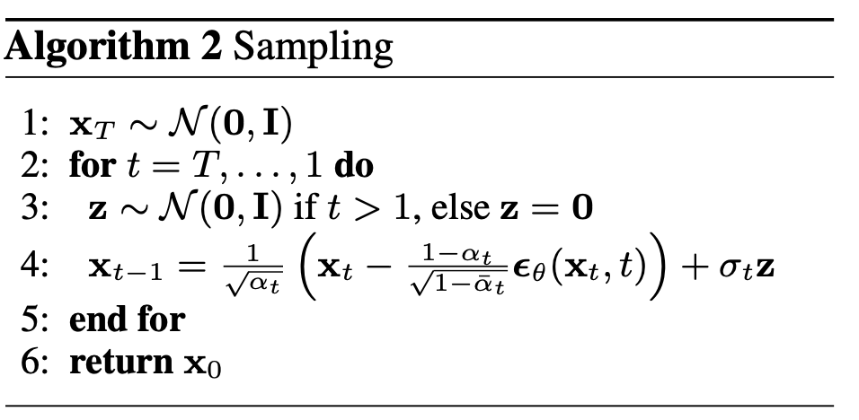
After training and obtaining the denoising network \(\epsilon_\theta (x_t, t)\), we can approximate \(\tilde{\mu} (x_t, x_0) \approx \mu_\theta(x_t, t) = \frac{1}{\sqrt{\alpha_t}} \left( x_t - \frac{1 - \alpha_t}{\sqrt{1 - \bar{\alpha}_t}} \epsilon_\theta (x_t, t) \right)\).
So, the final equation to sample \(x_{t-1}\) for us ![]() is:
is:
where \(z \sim \mathcal{N}(0, I)\).
Implementation
Here is the embedded Jupyter notebook.