A Tutorial on Diffusion Models (Part 2)
DDIM, Diffusion Inversion and Accelerating Inference
Resources
- The Jupyter notebooks associated with this tutorial can be found here.
- The first part of this tutorial can be found here.
- FastAI tutorial about DDIM can be found here.
DDIM
One of the main drawbacks of DDPM is that training process requires a large \(T\) to reach the equilibrium state. In inference, to obtain a sample \(x_0\), we need to run through \(T\) reverse steps, sequentially, which is very slow. To address this issue, Song et al.
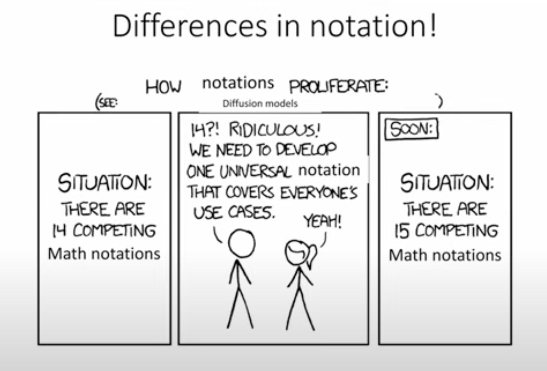
Change of Notation

| DDPM | DDIM | |
|---|---|---|
|
atomic param |
\(0 < \alpha_t < 1, \beta_t = 1 - \alpha_t\) | \(0 < \bar{\alpha}_t < 1, \beta_t = 1 - \bar{\alpha}_t\) |
| cummulative param | \(\bar{\alpha}_t = \prod_{i=1}^{t} \alpha_i\) | \(\alpha_t = \prod_{i=1}^{t} \bar{\alpha}_i\) |
| \(q(x_t \mid x_{t-1})\) | \(\mathcal{N} (x_t; \sqrt{\alpha_t} x_t, (1 - \alpha_t) I)\) | \(\mathcal{N} (x_t; \sqrt{\frac{\alpha_t}{\alpha_{t-1}}}x_{t-1}, (1 - \frac{\alpha_t}{\alpha_{t-1}})I)\) \(^{\star}\) |
| \(q(x_t \mid x_0)\) | \(\mathcal{N} (x_t; \sqrt{\bar{\alpha}_t} x_0, (1 - \bar{\alpha}_t) I)\) | \(\mathcal{N} (x_t; \sqrt{\alpha_t} x_0, (1 - \alpha_t) I)\) |
| (forward) sampling \(x_t\) | \(x_t = \sqrt{\bar{\alpha}_t} x_0 + \sqrt{1-\bar{\alpha}_t} \epsilon\) | \(x_t = \sqrt{\alpha_t} x_0 + \sqrt{1-\alpha_t} \epsilon\) |
| (reverse) sampling \(x_{t-1}\) | \(\frac{1}{\sqrt{\alpha_t}} \left( x_t - \frac{1 - \alpha_t}{\sqrt{1 - \bar{\alpha}_t}} \epsilon_\theta (x_t, t) \right) + \sigma_t z\) | \(\frac{1}{\sqrt{\bar{\alpha}_t}} \left( x_t - \frac{1 - \bar{\alpha}_t}{\sqrt{1 - \alpha_t}} \epsilon_\theta (x_t, t) \right) + \sigma_t z\) |
| \(\sigma_t\) | \(\frac{1 - \bar{\alpha}_{t-1}}{1 - \bar{\alpha}_t}\) | \(\frac{1 - \alpha_{t-1}}{1 - \alpha_t}\) |
\(^{\star}\) In the DDIM paper, the authors made a note that covariance matrix is ensured to have positive terms on its diagonal. The \(\alpha_{1:T} \in (0, 1]^T\) is a decreasing sequence, i.e., \(\alpha_{t+1} \leq \alpha_t\), \(\alpha_1 = 1\) and \(\alpha_T \approx 0\) where \(T \rightarrow \infty\).
With this in mind, I believe that the variable naming in the LDM implementation (which can be found here: https://github.com/Stability-AI/stablediffusion/blob/main/ldm/models/diffusion/ddpm.py cannot confuse you anymore ![]() .
.
    to_torch = partial(torch.tensor, dtype=torch.float32)

    self.register_buffer('betas', to_torch(betas))
    self.register_buffer('alphas_cumprod', to_torch(alphas_cumprod))
    self.register_buffer('alphas_cumprod_prev', to_torch(alphas_cumprod_prev))

    # calculations for diffusion q(x_t | x_{t-1}) and others
    self.register_buffer('sqrt_alphas_cumprod', to_torch(np.sqrt(alphas_cumprod)))
    self.register_buffer('sqrt_one_minus_alphas_cumprod', to_torch(np.sqrt(1. - alphas_cumprod)))
    self.register_buffer('log_one_minus_alphas_cumprod', to_torch(np.log(1. - alphas_cumprod)))
    self.register_buffer('sqrt_recip_alphas_cumprod', to_torch(np.sqrt(1. / alphas_cumprod)))
    self.register_buffer('sqrt_recipm1_alphas_cumprod', to_torch(np.sqrt(1. / alphas_cumprod - 1)))
Fortunately, in the implementation of DDIM, the authors keep the same notation of the DDPM implementation and introduce some new variables just for the DDIM model.
    # ddim sampling parameters
    ddim_sigmas, ddim_alphas, ddim_alphas_prev = make_ddim_sampling_parameters(alphacums=alphas_cumprod.cpu(),
                                                                                ddim_timesteps=self.ddim_timesteps,
                                                                                eta=ddim_eta,verbose=verbose)
    self.register_buffer('ddim_sigmas', ddim_sigmas)
    self.register_buffer('ddim_alphas', ddim_alphas)
    self.register_buffer('ddim_alphas_prev', ddim_alphas_prev)
    self.register_buffer('ddim_sqrt_one_minus_alphas', np.sqrt(1. - ddim_alphas))
    sigmas_for_original_sampling_steps = ddim_eta * torch.sqrt(
        (1 - self.alphas_cumprod_prev) / (1 - self.alphas_cumprod) * (
                    1 - self.alphas_cumprod / self.alphas_cumprod_prev))
Diffusion Inversion

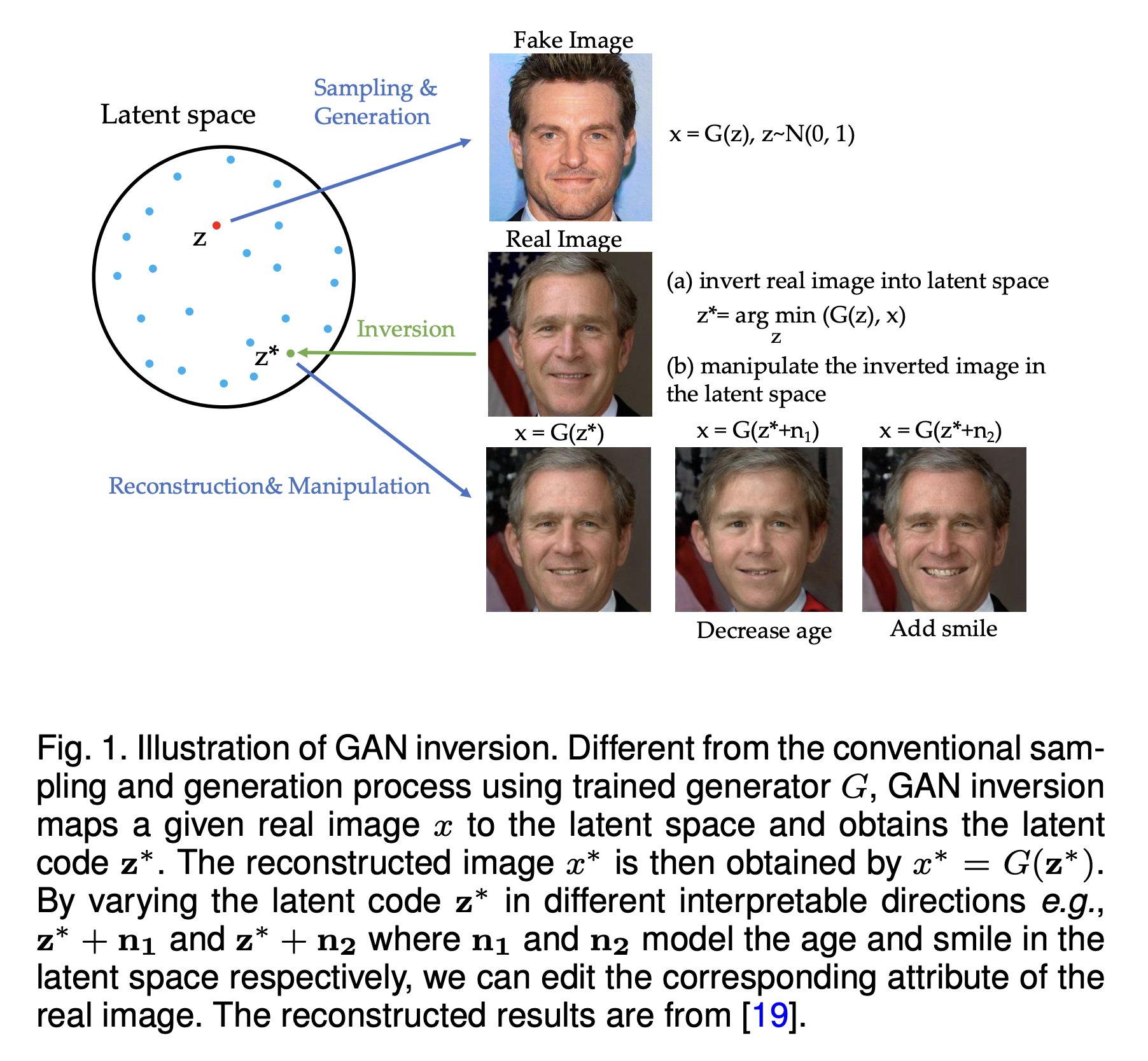
Generative inversion is a technique that allows us to invert the generation process. In other words, given a pre-trained generative model \(g_\theta(z)\) and an image \(x\) which can be either real image or generated one, we can find the noise \(z\) such that \(g_\theta(z)\) is close to \(x\). This technique was first proposed for GANs in Zhu et al. (2016)
Because requring the deterministic property: one noise \(z\) always generates the same image \(x\), this technique is not trivial to apply to other generative models such as VAEs or Flow-based models. For Diffusion Models, thanks to the deterministic property in DDIM, we can apply this technique to invert the diffusion process, i.e., given an image \(x_0\), we can find the noise \(x_T\) to reconstruct \(x_0\). And with the blooming of Diffusion Models in the last two years, we can see many cool applications of this technique such as Textual Inversion
In the DDPM framework, the forward diffusion process has a nice property that:
\[x_t = \sqrt{\bar{\alpha}_t} x_0 + \sqrt{1-\bar{\alpha}_t} \epsilon_t\]where \(x_0\) is the initial image, \(\epsilon_t \sim \mathcal{N}(0, I)\) is the noise at time \(t\). This property allows us to predict noisy version \(x_t\) of \(x_0\) at any arbitrary time \(t\). On the other hand, given \(\epsilon_t = \epsilon_\theta(x_t, t)\) is the predicted noise at time \(t\) by the denoising network \(\epsilon_\theta\) and \(x_t\), we can predict \(\tilde{x}_0\) as follows:
\[\tilde{x}_0 = \frac{x_t - \sqrt{1-\bar{\alpha}_t} \epsilon_\theta(x_t, t)}{\sqrt{\bar{\alpha}_t}}\]Now we consider the next step in the forward diffusion process:
\[x_{t+1} = \sqrt{\bar{\alpha}_{t+1}} x_0 + \sqrt{1 - \bar{\alpha}_{t+1}} \epsilon_{t+1}\]where \(\epsilon_{t+1} \sim \mathcal{N}(0, I)\) is the noise at time \(t+1\). If we replace the original \(x_0\) with the predicted \(\tilde{x}_0\) and assume that the diffusion process is large enough so that \(\epsilon_{t+1} \approx \epsilon_\theta(x_t, t)\), we can obtain the inverted diffusion process as follows:
\[x_{t+1} = \sqrt{\bar{\alpha}_{t+1}} \frac{x_t - \sqrt{1-\bar{\alpha}_t} \epsilon_\theta(x_t, t)}{\sqrt{\bar{\alpha}_t}} + \sqrt{1 - \bar{\alpha}_{t+1}} \epsilon_\theta(x_t, t)\]which now depends only on \(x_t\) and \(\epsilon_\theta(x_t, t)\). Repeating this process from \(t=0\) to \(t=T\), we can obtain the inverted code \(x_T\) that reconstructs \(x_0\) (again it works for DDIM model only).
Implementation
Jumping Prediction
In this demo, I will show you one of the applications of diffusion inversion - jumping prediction. The goal is to predict the initial image \(x_0\) from the image \(x_t\) at any arbitrary time \(t\) in the diffusion process. It can be done by using the following equation:
\[\tilde{x}_0 = \frac{x_t - \sqrt{1-\bar{\alpha}_t} \epsilon_\theta(x_t, t)}{\sqrt{\bar{\alpha}_t}}\]where \(\tilde{x}_0\) is the predicted image at time \(t=0\) given the image \(x_t\) at time \(t\) and the noise \(\epsilon_\theta(x_t, t)\).
Why care about this?
Standard Diffusion Model In the first part, I use the Guided-Diffusion by OpenAI as the codebase to demonstrate this technique (i.e., predicting \(x_0\) from \(x_t\)). The codebase is for the Diffusion Models Beat GANS on Image Synthesis paper. I have blogged about this paper and some important components of the codebase here.
The main function to predict \(x_0\) from \(x_t\) as follows:
    def pred_eps_and_x0_from_xstart_uncond(model_fn, diffusion, x_start, t, y=None):
        """
        the (uncondition/standard) $$\epsilon_\theta(x_t,t)$$
        the (uncondition/standard) $$\tilde{x}_0 = \frac{x_t - \sqrt{1 - \bar{\alpha}_t} \epsilon_\theta(x_t,t)}{\sqrt{\bar{\alpha}_t}}$$
        note 1: the _predict_xstart_from_eps() function does not have parameter, therefore, using auxiliary_diffusion or diffusion does not matter
        """
        assert y is not None
        B, C = x_start.shape[:2]
        assert t.shape == (B,)
        noise = th.randn_like(x_start)
        x_t = diffusion.q_sample(x_start, t, noise=noise)
        eps = model_fn(x_t, diffusion._scale_timesteps(t), y) # only this step has trainable parameter
        assert eps.shape == (B, C * 2, *x_start.shape[2:])
        eps, _ = th.split(eps, C, dim=1)

        x_0 = diffusion._predict_xstart_from_eps(x_t, t, eps)
        return eps, x_0
    def pred_eps_and_x0_from_xstart_cond(model_fn, diffusion, cond_fn, x_start, t, y=None):
        """
        the condition $$\hat{\epsilon}_{\theta}(x_t,t,y,\phi) = \epsilon_\theta(x_t,t) - \sqrt{1 - \bar{\alpha}_t} \nabla_{x_t} \log p_\phi (y \mid x_t)$$ as in classifier-guidance model
        the condition $$\tilde{x}_0 = \frac{x_t - \sqrt{1 - \bar{\alpha}_t} \hat{\epsilon}_{\theta}(x_t,t,y,\phi)}{\sqrt{\bar{\alpha}_t}}$$
        note 1: the _predict_xstart_from_eps() function does not have parameter, therefore, using auxiliary_diffusion or diffusion does not matter
        note 2: the classifier should be the ORIGINAL classifier, not the auxiliary classifier
        """
        assert y is not None
        B, C = x_start.shape[:2]
        assert t.shape == (B,)
        alpha_bar = _extract_into_tensor(diffusion.alphas_cumprod, t, x_start.shape)
        noise = th.randn_like(x_start)
        x_t = diffusion.q_sample(x_start, t, noise=noise)
        eps = model_fn(x_t, diffusion._scale_timesteps(t), y) # only this step has trainable parameter
        assert eps.shape == (B, C * 2, *x_start.shape[2:])
        eps, _ = th.split(eps, C, dim=1)
        grad = cond_fn(x_t, diffusion._scale_timesteps(t), y)
        eps = eps - (1 - alpha_bar).sqrt() * grad
        x_0 = diffusion._predict_xstart_from_eps(x_t, t, eps)
        return eps, x_0
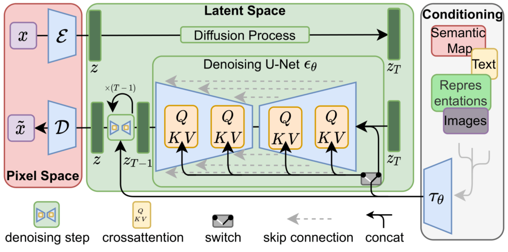
Latent Diffusion Model Unlike the previous codebase, the latent diffusion model has three main components: encoder \(\mathcal{E}\) and decoder \(\mathcal{D}\), U-Net \(\epsilon_\theta\), and the conditioning mechanism \(\tau\), in which the diffusion process is on the latent space instead of the image space.

Therefore, to make a prediction of \(x_0\) from \(x_t\) we need the following steps:
Step 1: Getting \(z_t\). There are two ways to obtain \(z_t\):
- Using forward process given \(x_0\) as \(z_t = \sqrt{\bar{\alpha}_t} z_0 + \sqrt{1-\bar{\alpha}_t} \epsilon_t\) where \(z_0 = \mathcal{E}(x_0)\) is the latent code of the input image \(x_0\), and \(\epsilon_t \sim \mathcal{N}(0, I)\) is the noise at time \(t\).
- Using the reverse process given \(z_T\) and a prompt \(c\) as \(z_{t-1} = \frac{1}{\sqrt{\alpha_t}} (z_{t+1} - \frac{1 - \alpha_t}{\sqrt{1-\bar{\alpha}_t}} \epsilon_\theta (z_{t+1}, t, \tau(c))) + \sigma_t \epsilon\) where \(\epsilon\) is the noise. It is important to note that we consider the conditional diffusion process, i.e., \(\epsilon_\theta (z_{t+1}, t, \tau(c))\) where \(\tau(c)\) is the embedding vector of the prompt \(c\).
Step 2: Predict the latent code \(z_0\) from \(z_t\) using a similar equation as in the standard diffusion model. However, again, we need to consider the conditional diffusion process.
\[\tilde{z}_0 = \frac{z_t - \sqrt{1-\bar{\alpha}_t} \epsilon_\theta(z_t, t, \tau(c))}{\sqrt{\bar{\alpha}_t}}\]Step 3: Using the decoder to obtain the image \(x_0\) from \(z_0\).
\[\tilde{x}_0 = \mathcal{D}(\tilde{z}_0)\]It is a worth noting that, in the inference process of the LDM (with diffusers) (which can be found in the generate-images.py) in each inference step, the U-Net outputs the unconditional noise \(\epsilon_u\) and the conditional noise \(\epsilon_c\). And the final noise \(\epsilon = \epsilon_u + \text{guidance_scale} (\epsilon_c - \epsilon_u)\) is used to sample the next latent code \(z_{t+1}\).
Notebooks
Here is the embedded Jupyter notebook. The result is really interesting. In this example, I use a prompt Image of cassette player to generate images with Stable Diffusion version 1.4 with DDIM and 100 steps. Each row shows the Predicted image \(\tilde{x}_0 = \mathcal{D}(\tilde{z}_0)\), Generated image using the current latent code \(\tilde{x}_t = \mathcal{D}(\tilde{z}_t)\), and Scaled Difference between two images \(\delta = \frac{\tilde{x}_0 - \tilde{x}_t}{\max (\tilde{x}_0 - \tilde{x}_t)}\), respectively.
We can see that, at early steps (i.e., \(t > 80\)) the two images look very noisy and do not show any sign of desired object in the prompt. However, if looking to the difference image (i.e., delta), we can still see some patterns of the object. It shows that the prediction technique works even at very early steps of the diffusion process. And, through the diffusion process, the difference becomes smaller and smaller and the two images nearly identical at the end of the process.