Tree-Ring Watermarks - Fingerprints for Diffusion Images that are Invisible and Robust
How to know whether an image is real or fake?
About the paper
- Published at NeurIPS 2023
- Affiliation: University of Maryland. Tom Goldstein’s group
- Link to the paper: https://arxiv.org/pdf/2305.20030.pdf
- Link to Github: https://github.com/YuxinWenRick/tree-ring-watermark
- Link to Yannic Kilcher’s video: https://youtu.be/WncUlZYpdq4?si=thX3fiKHS59SQ1IG
Side information: Tom is one of the most famous and active researchers in the field of Trustworthy Machine Learning, particulaly Adversarial Machine Learning.
His group has published several notable papers, such as Invisible Cloak
Summary:
- Problem setting: How to insert a watermark into a generated image such that the watermark is robust to the attack and invisible to the human eye?
- Approach: The authors proposed a simple yet effective watermarking framework for diffusion models which consits generation phase and detection phase. The method is based on the idea of diffusion inversion which allows us to invert the diffusion process. The key idea is to embed a watermark into the initial noise in frequency domain and then use the diffusion inversion to extract the watermark from the generated image in detection phase.
- Pros: The approach doesn’t require to change the weight of the diffusion model but just need to modify the input noise. Therefore, every user can have their own secret watermarking without changing the model.
- Cons: The method is evaluated under a quite weak black-box attack. This method is only applicable to DDIM (deterministic version of DDPM) and not applicable to other generative models such as VAEs or Flow-based models.
Follow-up ideas:
- How to fine-tune the foundation model (i.e., Stable Diffusion which does not have the watermark) to a new model with watermarking capability naturally? In this case, every generated output will have secret watermarking and from that we now can know whether an image is real or fake!
- How about stochastic diffusion model like DDPM?
After all, we still don’t know whether an image is real or fake ![]() .
.
Background
Watermarking
What is Watermarking? Watermarking is a technique to embed some information into a signal (image, audio, video, etc.) in a way that the signal is not changed much, but the information can be extracted later. The information can be used for many purposes, such as authentication, copyright.
Watermarking: Attack and Defense Game The watermarking process can be seen as an adversarial game between two parties: attacker and defender. The attacker tries to remove the watermark from the signal, while the defender tries to make the watermark robust to the attacker’s removal process. The game is illustrated in the following figure.
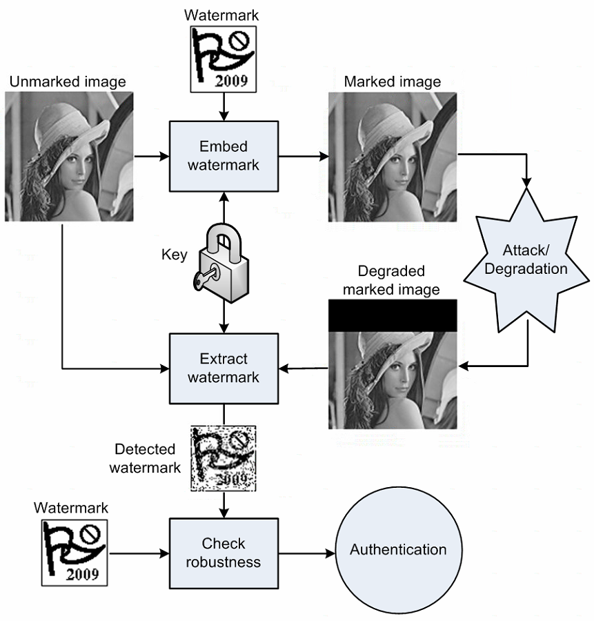
The defender has two main goals: (1) to make the watermark robust to the attacker’s removal process, and (2) to make the watermark invisible to the human eye. The first goal is measured by the robustness of the watermark, while the second goal is measured by the fidelity of the watermark. Similar as the trade-off between accuracy and robustness in the adversarial machine learning, the robustness and fidelity are usually conflicting, i.e., the more robust the watermark is, the more visible it is.
To extract the watermark, the defender needs a secret key and a secret decoder which are usually known only to the defender. There are two types of attack settings: white-box and black-box attacks depending on whether the attacker knows the secret key and decoder or not. Again, similar as the adversarial machine learning, the white-box attack is usually more powerful but less practical than the black-box attack.
Adaptive Attack is a special type of attack where the attacker knows everything about the defender, i.e., the secret key, decoder, and the defense algorithm and can adaptively change the attack strategy based on the defender’s strategy. This type of attack is usually the most powerful and the most difficult to defend (and almost impossible to defend in the adversarial machine learning). In this paper, the authors evaluated their method under non-adaptive white-box attack.
Why Watermarking in Generative Models? Originally, watermarking is to protect the ownership of the authors on their digital products. However, in the context of generative models, where a product is generated from a model with users’ input, the ownership is not clear. And when digging deeper, I found that copyright of AI art is complicated. Some important points that I got from this article WHO OWNS AI-GENERATED CONTENT? UNDERSTANDING OWNERSHIP, COPYRIGHTING, AND HOW THE LAW INTERPRETS AI-GENERATED ART
- According to (US) copyright law, only humans can be granted copyrights. If it’s created by AI, nobody can claim ownership of it or copyright it.
- But, if a person uses AI as a tool and gives very distinct/creative inputs in the process to create something, then the person can (again, as my understanding) claim ownership of the final product. For example, as mentioned in the arcticle,
graphic-novel artist Kris Kashtanova was granted copyright for their AI-generated comic book “Zarya of the Dawn” for the simple reason that there was human input in creating the entire comic book and its underlying storyline. The entire comic book was “AI-assisted” and not “AI-generated”, which is why it was eligible for copyright. - Specific to text-to-image models as Stable Diffusion, Dall-E, MidJourney, etc, the answer depends from case to case and if you care about the ownership, the first thing to do is read the
Terms and Conditonscarefully. In general, there are common points from these models:- User own all Assets the user create with the Services, to the extent possible under current law.
- However, user’s input (e.g., text prompt, input images) is granted to the company to use to improve and maintain their services.
- User is responsible for the content and ensuring that it does not violate any laws or intellectual property rights
Now, given the above points, back to the question: Why Watermarking in Generative Models?, I think the main purpose of the watermarking is to protect the ownership of the users on their generated products.
However, it is a much more interesting implication of watermarking in generative models than just authentication. If we can robustly and reliably detect a watermark in a generated image, we can know whether the image is real or fake, which is a very important problem in the field of Trustworthy Machine Learning.
What is DFT and why watermarking loves DFT?
Reference: https://vincmazet.github.io/bip/filtering/fourier.html and https://www.cs.unm.edu/~brayer/vision/fourier.html
As studied in the classical watermarking literature, the watermarking process is usually done in the frequency domain. Some important points about the frequency domain are (to my understanding):
- Modification in the frequency domain is more robust to image transformation such as rotation, translation, scaling, etc. than modification in the spatial domain (ref)
- Modification in the frequency domain is easier to make the watermark invisible to the human eye. DFT transformation converts an image to a phase and an amplitude. The amplitude represents the intensity of the different frequencies in the image while the phase represents the location of the frequencies. The human vision comprehends the shape of an object better than its intensity, therefore, the phase is more important than the amplitude. This is the reason why we can remove/add the watermark by modifying the amplitude while keeping the phase unchanged.
Diffusion Inversion
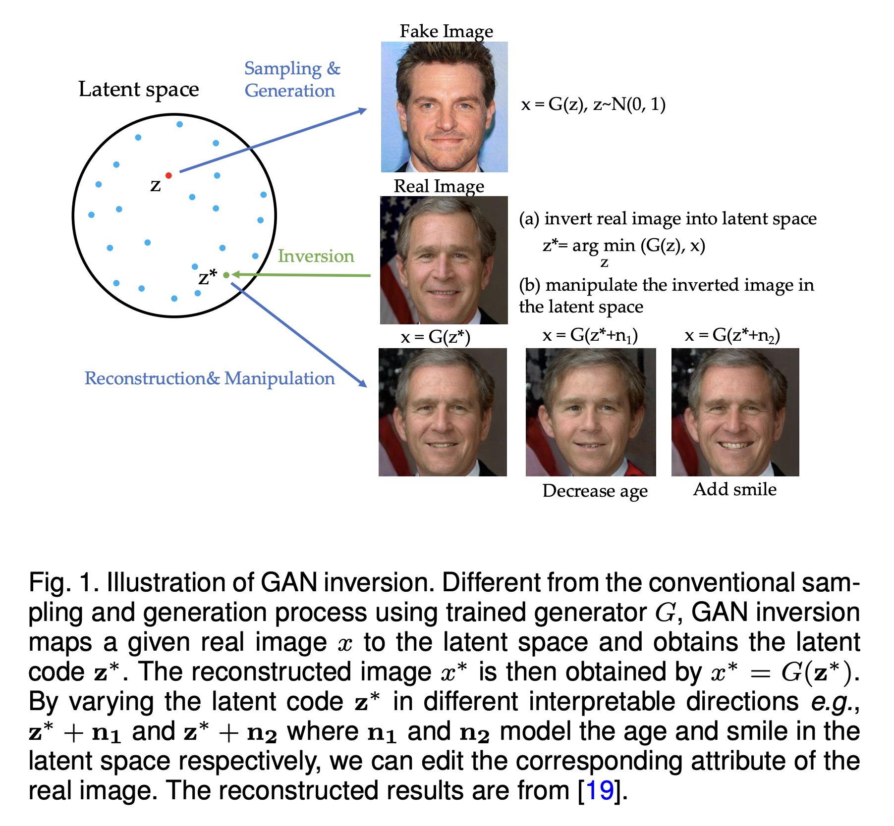
Generative inversion is a technique that allows us to invert the generation process. In other words, given a pre-trained generative model \(g_\theta(z)\) and an image \(x\) which can be either real image or generated one, we can find the noise \(z\) such that \(g_\theta(z)\) is close to \(x\). This technique was first proposed for GANs in Zhu et al. (2016)
Because requring the deterministic property: one noise \(z\) always generates the same image \(x\), this technique is not trivial to apply to other generative models such as VAEs or Flow-based models. For Diffusion Models, thanks to the deterministic property in DDIM, we can apply this technique to invert the diffusion process, i.e., given an image \(x_0\), we can find the noise \(x_T\) to reconstruct \(x_0\). And with the blooming of Diffusion Models in the last two years, we can see many cool applications of this technique such as Textual Inversion
In the DDPM framework, the forward diffusion process has a nice property that:
\[x_t = \sqrt{\bar{\alpha}_t} x_0 + \sqrt{1-\bar{\alpha}_t} \epsilon_t\]where \(x_0\) is the initial image, \(\epsilon_t \sim \mathcal{N}(0, I)\) is the noise at time \(t\). This property allows us to predict noisy version of \(x_0\) at any arbitrary time \(t\). On the other hand, given \(\epsilon_t = \epsilon_\theta(x_t, t)\) is the predicted noise at time \(t\) by the denoising network \(\epsilon_\theta\) and \(x_t\), we can predict \(\tilde{x_0}\) as follows:
Now we consider the next step in the forward diffusion process:
\[x_{t+1} = \sqrt{\bar{\alpha}_{t+1}} x_0 + \sqrt{1 - \bar{\alpha}_{t+1}} \epsilon_{t+1}\]where \(\epsilon_{t+1} \sim \mathcal{N}(0, I)\) is the noise at time \(t+1\). If we replace the original \(x_0\) with the predicted \(\tilde{x}_0\) and assume that the diffusion process is large enough so that \(\epsilon_{t+1} \approx \epsilon_\theta(x_t, t)\), we can obtain the inverted diffusion process as follows:
\[x_{t+1} = \sqrt{\bar{\alpha}_{t+1}} \frac{x_t - \sqrt{1-\bar{\alpha}_t} \epsilon_\theta(x_t, t)}{\sqrt{\bar{\alpha}_t}} + \sqrt{1 - \bar{\alpha}_{t+1}} \epsilon_\theta(x_t, t)\]which now depends only on \(x_t\) and \(\epsilon_\theta(x_t, t)\). Repeating this process from \(t=0\) to \(t=T\), we can obtain the inverted code \(x_T\) that reconstructs \(x_0\) (again it works for DDIM model only). This is the key technique used in this watermarking method.
Tree-Ring Watermark
Threat Model
In adversarial machine learning, a threat model is a description of capabilities and objectives of all parties in the attack and defense game. From that, we can narrow down the defense space and scope to this specific threat model (It is because in the real world, we cannot know every possible attack and defend against it). In this paper, the authors considered the following threat model:
- Model owner (generative phase): The generative model owner generates an image \(x\) with a secret watermark \(k\). The constraint is that the watermarking algorithm should have a negligible effect on the generation process, so that quality is maintained and watermarking leaves no visible trace.
- Attacker or Forger (attack phase): The attacker tries to remove the watermark from the generated image \(x\) to get \(x'\) (and then can claim his ownership on \(x'\), etc.). The attacker uses data augmentations only and knows nothing about the watermarking algorithm and the generative model (a quite weak black-box attack).
- Model owner (detection phase): The model owner tries to detect the watermark in the image \(x'\) to know whether it was modified from the original image \(x\) or not. The model owner knows nothing about the attack including its techniques and hyper-parameters.
Watermarking Process
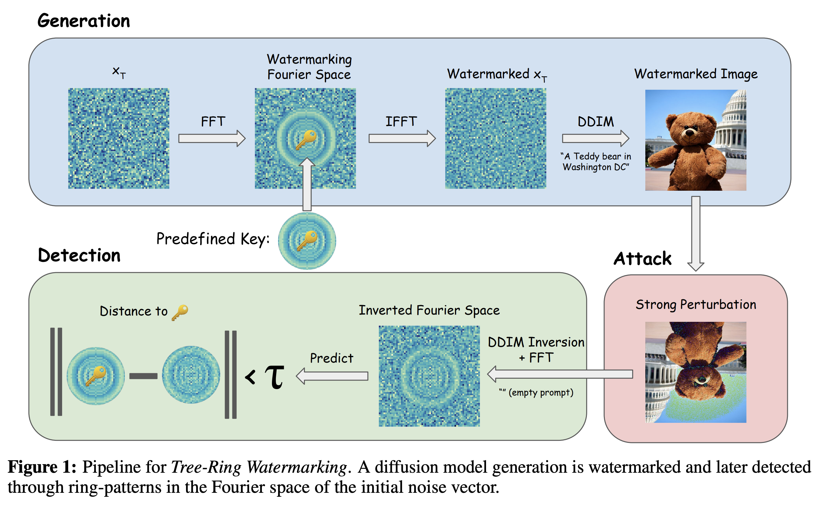
The watermarking process is illustrated in the above figure. The watermarking process consists of two main steps: watermark embedding and watermark detection.
In the watermark embedding step, an initial Gaussian noise \(x_T\) is first converted to the frequency domain using DFT \(\mathcal{F}\). Then, a pre-defined watermark \(k\) is embedded into the frequency domain of \(x_T\) by a simple binary masking operation. The watermarked noise \(x_T^k\) is then converted back to the time domain using inverse DFT \(\mathcal{IF}\). Finally, the watermarked noise \(x_T^k\) is used to generate the watermarked image \(x_0^k\) (now call \(x\)) using the standard DDIM model (again not stochastic one like DDPM).
In the watermark detection, the transformed image \(x'=\mathcal{A}(x_0^k)\) is first inverted to obtain the approximated noise \(x'_T\) using the DDIM inversion. Then, the watermark \(k'\) is extracted from the frequency domain of \(x'_T\) using the same binary masking operation as in the watermark embedding step. Finally, the extracted watermark \(k'\) is compared with the original watermark \(k\) to determine whether the image \(x'\) is from the original image \(x\) or not.
The simple process can be describe as follows:
Watermark Embedding
Input: initial noise \(x_T\), secret key \(k\), mask \(M\), DDIM model \(\mathcal{D}\)
\(x_T^f = \mathcal{F}(x_T)\)
\(x_T^k = Masking(x_T^f, k, M)\)
\(x_0^k = \mathcal{D}(\mathcal{IF}(x_T^k))\)
Output: watermarked image \(x_0^k\) or \(x\)
Watermark Detection
Input: transformed image \(x'\), secret key \(k\), mask \(M\), DDIM inversion \(\mathcal{D}^I\)
\(x'_T = \mathcal{D}^I (x')\)
\({x'}_T^f = \mathcal{F}(x'_T)\)
\(k' = UnMasking({x'}_T^f, k, M)\)
calculate distance \(d(k, k')\) between \(k'\) and \(k\)
Output: \(d(k, k')\)
As described in the paper, the masking opearation will produce output:
\[x_{i,T}^k \sim \left\{ \begin{array}{ c l } k_i & \quad \textrm{if } i \in M \\ \mathcal{N} (0,1) & \quad \textrm{otherwise} \end{array} \right.\]where \(k_i\) is the \(i\)-th element of the key \(k\), \(M\) is the mask. Note that the Fourier transform of a Gaussian noise array is also distributed as Gaussian noise. The distance function is the L1 distance \(d(k, k') = \frac{1}{\mid M \mid} \sum_{i \in M} \mid k_i - k'_i \mid\).
Constructing the key
As mentioned in the paper, choosing the key pattern \(k\) (as similar the binary mask \(M\)) strongly effects the robustness and visibility of the watermark. The authors proposed to use a tree-ring pattern which is a circular mask with radius \(r\) centered on the low frequency modes as the key pattern. This pattern brings several benefits such as invariant to rotation, translation, and dilation (which was studied in classical watermarking literature). The authors proposed three variants of the tree-ring pattern:
- Tree-ring Zero: all elements in the tree-ring pattern are zero.
- Tree-ring Rands: all elements in the tree-ring pattern are randomly sampled from \(\mathcal{N}(0,1)\).
- Tree-ring Rings: multiple rings with different radiuses.
Why ring pattern?
How to detect the watermark?
Given an image \(x'\) and from the watermark detection process, we can obtain \(k'\) which is the extracted pattern from \(x'\). Now, how we can decide whether \(k'\) is the same as the original pattern \(k\) or not?
To do that, the authors defined a null hypothesis \(H_0\) and find the P-value of the null hypothesis. The null hypothesis is defined as follows:
\[H_0: k' \sim \mathcal{N}(0, \sigma^2 I)\]Here, the variance \(\sigma^2\) is unknown and be estimated from each image as \(\sigma^2 = \frac{1}{\mid M \mid} \sum_{i \in M} \mid k'_i \mid^2\).
What is Null Hypothesis?
Null hypothesis is the claim that no relationship exists between two sets of data or variables being analyzed. For example, in the context of watermarking, the null hypothesis is a statement that the extracted pattern \(k'\) is just a random noise and not related to the original pattern \(k\). On the other hand, the alternative hypothesis is a statement that the extracted pattern \(k'\) is related to the original pattern \(k\).
What is P-value?
The P-value is the probability of obtaining results as extreme as the observed results of a statistical hypothesis test, assuming that the null hypothesis is correct. The smaller the P-value, the stronger the evidence against the null hypothesis. The P-value is calculated from the null hypothesis and the observed data using a statistical test. For example, in the context of watermarking, the P-value is the probability of obtaining the extracted pattern \(k'\) from the null hypothesis \(H_0\).
The P-value is calculated as follows:
\[p = Pr \left( \chi^2_{\mid M \mid, \lambda} \leq \eta \mid H_0 \right) = \Phi_{\chi^2} (z)\]where \(\chi^2_{\mid M \mid, \lambda}\) is the chi-squared distribution with \(\mid M \mid\) degrees of freedom and non-centrality parameter \(\lambda\), \(\eta = \frac{1}{\sigma^2} \sum_{i \in M} \mid k_i - k'_i \mid^2\), \(z = \frac{\eta - \lambda}{\sqrt{2 \lambda}}\), and \(\Phi_{\chi^2}\) is the cumulative distribution function of the chi-squared distribution.
From that, an image is considered as a forgery if \(p < \alpha\) where \(\alpha\) is a pre-defined threshold (too small \(\alpha\) will lead to many false positives, while too large \(\alpha\) will lead to many false negatives).
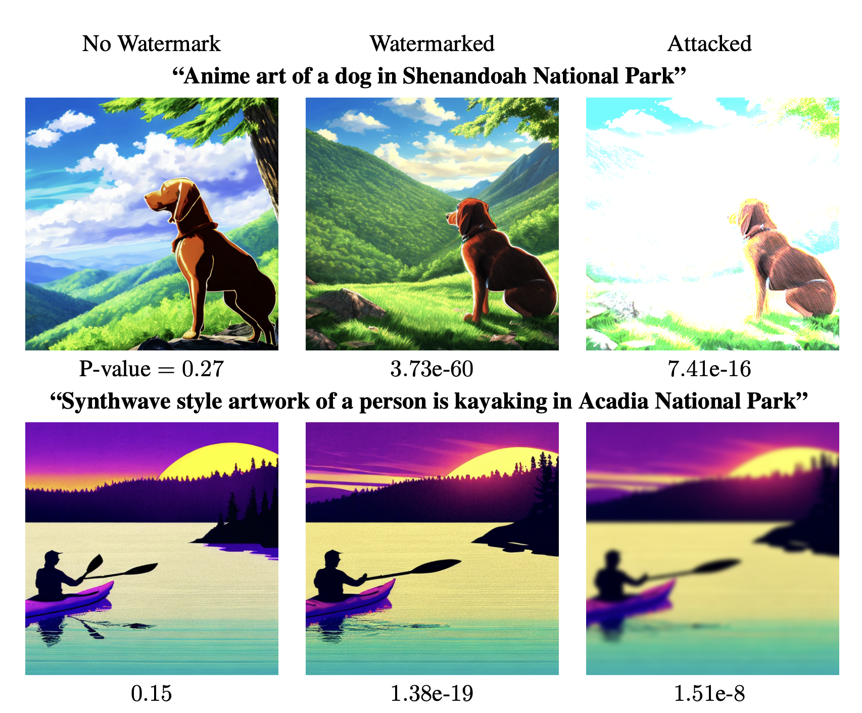
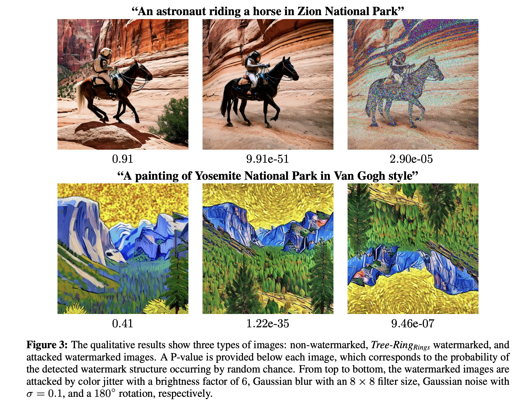
The figure above shows the P-value of the null hypothesis in three different settings including (1) without watermark, (2) with watermark, and (3) with watermark and attack. As we can see, the P-value of image with watermark is much lower than that of image without watermark, and the P-value in the last setting is extremely low, which indicates that the watermark is robust to the attack. The authors also provided a more quantitative analysis as Table 1 in the paper.
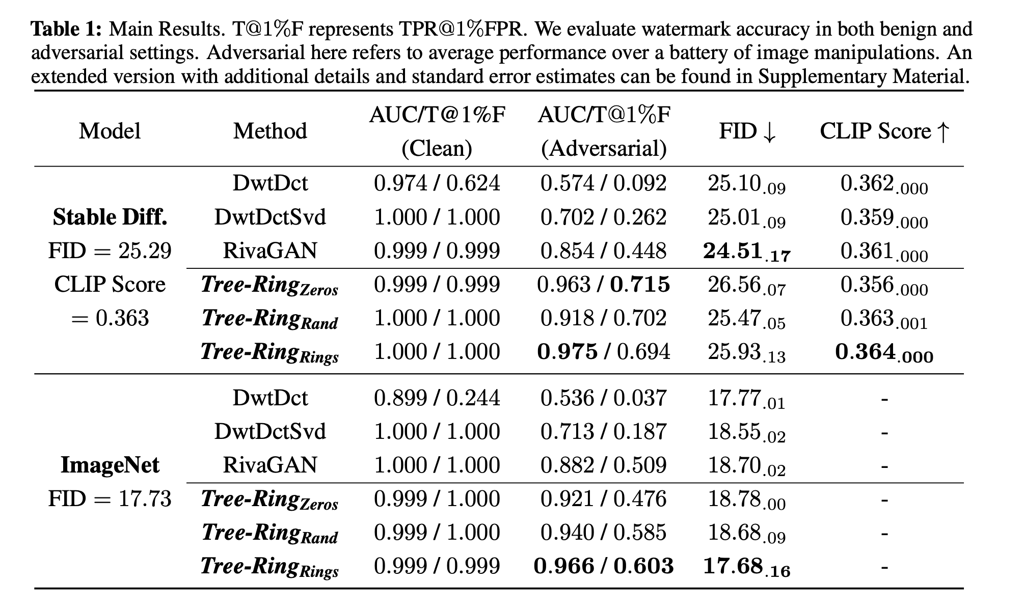
The metric was used to measure the performance is AUC/TPR@1%FPR which is the area under the ROC curve (AUC) or the true positive rate (TPR) at 1% false positive rate (FPR). The authors also used FID score to measure the quality of the generated images and CLIP score to measure the semantic similarity between the generated images and the prompts.
That’s all for the paper! There are still many experiments and analysis in the paper, but the post is already too long. Further details can be found in the paper.
Summary
Summary:
- Problem setting: How to insert a watermark into a generated image such that the watermark is robust to the attack and invisible to the human eye?
- Approach: The authors proposed a simple yet effective watermarking framework for diffusion models which consits generation phase and detection phase. The method is based on the idea of diffusion inversion which allows us to invert the diffusion process. The key idea is to embed a watermark into the initial noise in frequency domain and then use the diffusion inversion to extract the watermark from the generated image in detection phase.
- Pros: The approach doesn’t require to change the weight of the diffusion model but just need to modify the input noise. Therefore, every user can have their own secret watermarking without changing the model.
- Cons: The method is evaluated under a quite weak black-box attack. This method is only applicable to DDIM (deterministic version of DDPM) and not applicable to other generative models such as VAEs or Flow-based models.
Follow-up ideas:
- How to fine-tune the foundation model (i.e., Stable Diffusion which does not have the watermark) to a new model with watermarking capability naturally? In this case, every generated output will have secret watermarking and from that we now can know whether an image is real or fake!
- How about stochastic diffusion model like DDPM?