Foundations of Machine Learning
Most common machine learning interview questions
What is logistic regression?
Logistic regression is a statistical model that uses a logistic function to model the probability of a binary response based on one or more predictor variables. It is used for binary classification problems.
Mathematically, the logistic function is defined as:
\[P(Y=1|X) = \text{sigmoid} (W X + b)\]Where:
-
$$P(Y=1 X)$$ is the probability of the response variable Y being 1 given the input features X. - \(\text{sigmoid} (z) = \frac{1}{1 + e^{-z}}\) is the sigmoid function, which maps any real-valued number to the range [0, 1].
- \(W\) is the weight matrix and \(b\) is the bias vector. \(X\) has dimension \(n \times m\), where \(n\) is the number of features and \(m\) is the number of instances. \(W\) has dimension \(1 \times n\) and \(b\) has dimension \(1 \times m\).
What is the difference between supervised and unsupervised learning?
Supervised learning is a type of machine learning where the model is trained on a labeled dataset, meaning that the input data is paired with the correct output. The model learns to make predictions based on this labeled data. Unsupervised learning, on the other hand, is a type of machine learning where the model is trained on an unlabeled dataset, meaning that the input data is not paired with the correct output. The model learns to find patterns and structure in the data without explicit guidance.
What is overfitting and how can it be prevented?
Overfitting occurs when a model learns the training data too well, to the point that it performs poorly on new, unseen data. Overfitting can be prevented by using techniques such as cross-validation, regularization, and early stopping.
What is the bias-variance tradeoff?
The bias-variance tradeoff is a fundamental concept in machine learning that refers to the balance between bias and variance in a model. Bias refers to the error introduced by approximating a real-world problem with a simplified model, while variance refers to the error introduced by the model’s sensitivity to small fluctuations in the training data. The tradeoff arises because reducing bias typically increases variance, and vice versa.
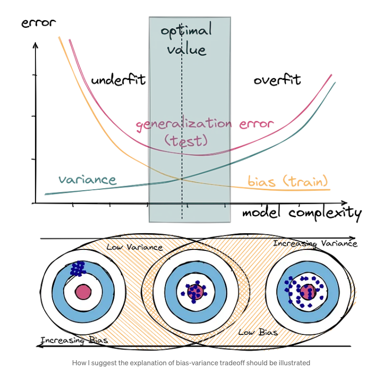
It is worth noting that in the image above, the variance is the spread of the model’s predictions around the mean, not the error on the validation set as we usually see in DL tutorials. The generalization error is the sum of the bias, variance, and irreducible error.
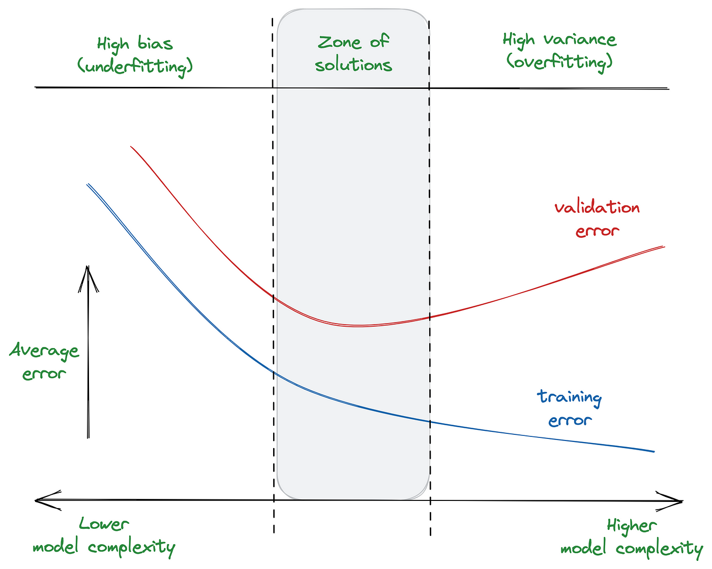
Mathematically, the generalization error can be decomposed into three components:
\[\text{Generalization error} = \text{Bias}^2 + \text{Variance} + \text{Irreducible error}\] \[\text{Bias} = \mathbb{E}[\hat{f}(x)] - f(x)\] \[\text{Variance} = \mathbb{E}[\hat{f}(x) - \mathbb{E}[\hat{f}(x)]]^2\]Reference: https://medium.com/@ivanreznikov/stop-using-the-same-image-in-bias-variance-trade-off-explanation-691997a94a54
What is the difference between classification and regression?
Classification is a type of supervised learning where the goal is to predict a discrete class label, such as “spam” or “not spam.” Regression, on the other hand, is a type of supervised learning where the goal is to predict a continuous value, such as a person’s age or the price of a house.
What is the difference between precision and recall?
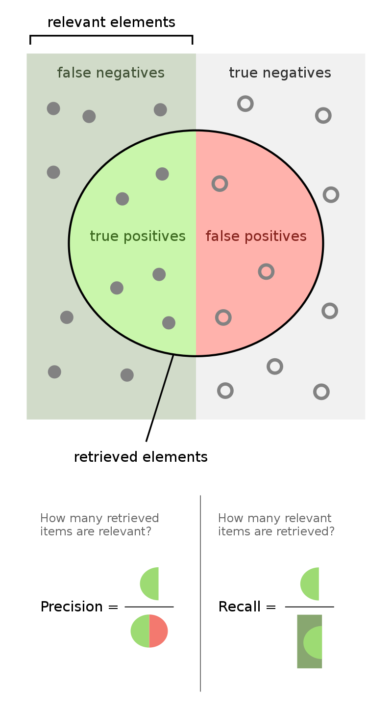
Precision is the ratio of true positive predictions to the total number of positive predictions, while recall is the ratio of true positive predictions to the total number of actual positive instances. Precision measures the accuracy of the positive predictions, while recall measures the ability of the model to find all the positive instances.
What is ROC curve?
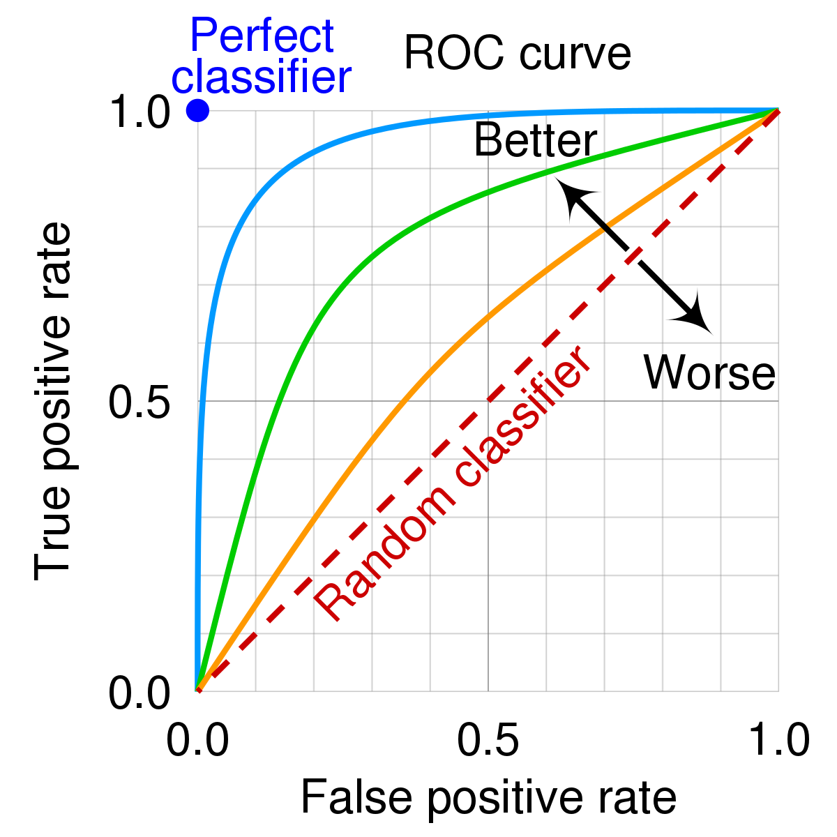
The ROC curve is a graphical representation of the tradeoff between the true positive rate (TPR) and the false positive rate (FPR) for a binary classification model. It is used to evaluate the performance of the model and to choose the optimal threshold for making predictions. Each point of the ROC curve represents a different threshold, and the area under the curve (AUC) is a measure of the model’s performance. The optimal threshold is the one that maximizes the TPR and minimizes the FPR. The best model is the one that has the highest AUC.
What is the difference between bagging and boosting?
Bagging and boosting are two ensemble learning techniques that combine multiple models to improve the overall performance. Bagging, or bootstrap aggregating, involves training multiple models on different subsets of the training data and then combining their predictions. Boosting, on the other hand, involves training multiple models sequentially, with each model focusing on the instances that were misclassified by the previous models. The main difference between bagging and boosting is the way the models are combined and the focus of each model.
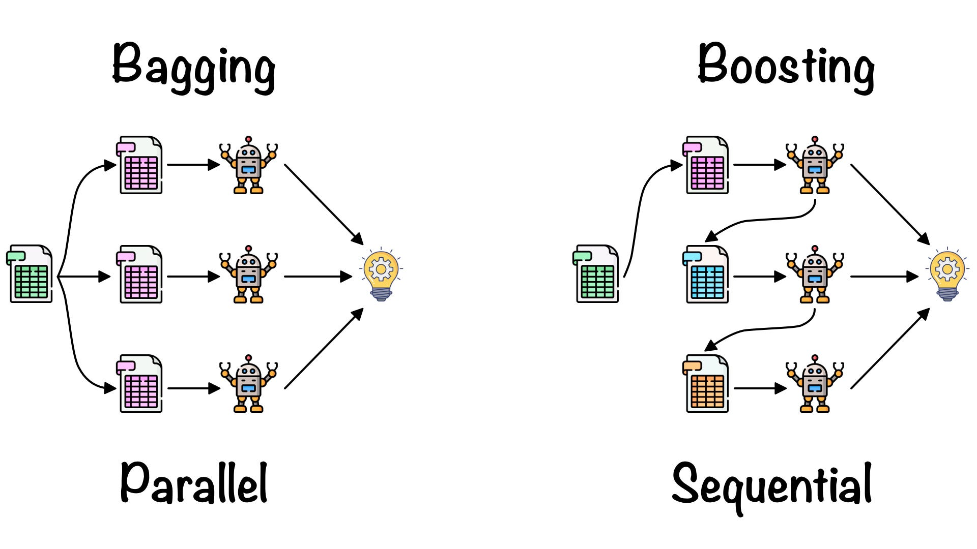
Reference: https://towardsdatascience.com/ensemble-learning-bagging-boosting-3098079e5422
What is the difference between a generative model and a discriminative model?
A generative model is a type of model that learns the joint probability distribution of the input features and the output labels, while a discriminative model is a type of model that learns the conditional probability distribution of the output labels given the input features. In other words, a generative model learns to generate new data, while a discriminative model learns to discriminate between different classes.
Mathematical explanation:
- Generative model: \(P(X, Y)\) where \(X\) is the input features and \(Y\) is the output labels. \(P(X, Y)\) is the joint probability distribution of X and Y.
-
Discriminative model: $$P(Y X)\(where\)X\(is the input features and\)Y\(is the output labels.\)P(Y X)$$ is the conditional probability distribution of Y given X. - Example: Naive Bayes is a generative model, while logistic regression is a discriminative model.
What is the difference between L1 and L2 regularization?
L1 and L2 regularization are two common techniques used to prevent overfitting in machine learning models. L1 regularization adds a penalty to the model’s loss function based on the absolute value of the model’s weights, while L2 regularization adds a penalty based on the squared value of the model’s weights. The main difference between L1 and L2 regularization is the type of penalty they impose on the model’s weights and the effect on the model’s sparsity.
L1 regularization:
- Adds a penalty based on the absolute value of the model’s weights.
- Encourages sparsity in the model’s weights, meaning that many of the weights will be set to zero.
- Useful for feature selection and reducing the number of features in the model.
- Example: Lasso regression.
-
Loss function: $$\mathcal{L}(\theta) + \lambda \sum_{i=1}^{n} \theta_i $$ - Gradient: \(\nabla_{\theta} \mathcal{L}(\theta) + \lambda \text{sign}(\theta)\)
- Update rule: \(\theta_{t+1} = \theta_t - \alpha \nabla_{\theta} \mathcal{L}(\theta) - \alpha \lambda \text{sign}(\theta)\)
L2 regularization:
- Adds a penalty based on the squared value of the model’s weights.
- Encourages small weights in the model, but does not force them to be exactly zero.
- Useful for preventing overfitting and improving the generalization of the model.
- Example: Ridge regression.
- Loss function: \(\mathcal{L}(\theta) + \lambda \sum_{i=1}^{n} \theta_i^2\)
- Gradient: \(\nabla_{\theta} \mathcal{L}(\theta) + 2 \lambda \theta\)
- Update rule: \(\theta_{t+1} = \theta_t - \alpha \nabla_{\theta} \mathcal{L}(\theta) - \alpha 2 \lambda \theta\)
- Note: The update rule for L2 regularization is also known as weight decay.
What is the difference between a hyperparameter and a parameter?
A hyperparameter is a configuration setting for a machine learning model that is set before the model is trained, while a parameter is a variable that is learned by the model during training. Hyperparameters are used to control the learning process and the structure of the model, while parameters are used to make predictions based on the input data.
Examples of hyperparameters:
- Learning rate
- Number of hidden layers
- Number of neurons in each layer
- Regularization strength
- Batch size
What is non-parametric machine learning?
Non-parametric machine learning refers to a class of machine learning models that do not make strong assumptions about the functional form of the underlying data distribution. Instead of estimating a fixed number of parameters, non-parametric models use the data to determine the number of parameters needed to represent the data. Non-parametric models are often more flexible and can capture complex patterns in the data, but they may require more data and computational resources.
On the other hand, parametric machine learning refers to a class of machine learning models that make strong assumptions about the functional form of the underlying data distribution. “A learning model that summarizes data with a set of parameters of fixed size (independent of the number of training examples) is called a parametric model. No matter how much data you throw at a parametric model, it won’t change its mind about how many parameters it needs.” (Artificial Intelligence: A Modern Approach, page 737).
Examples of non-parametric machine learning models:
- k-nearest neighbors (KNN)
- Decision trees
- Support vector machines (SVM)
Examples of parametric machine learning models:
- Linear regression
- Neural networks
What is k-nearest neighbors (KNN)?
K-nearest neighbors (KNN) is a simple and intuitive machine learning algorithm that is used for both classification and regression tasks. In KNN, the output of a new instance is predicted based on the majority class of its k-nearest neighbors. The distance between instances is typically measured using Euclidean distance, but other distance metrics can also be used.
Pseudocode for KNN:
- For each instance in the training data, calculate the distance between the new instance and the training instance.
- Select the k-nearest neighbors based on the distance metric.
- For classification tasks, predict the majority class of the k-nearest neighbors. For regression tasks, predict the average value of the k-nearest neighbors.
- Return the predicted output.
The K-nearest neighbor classification performance can often be significantly improved through (supervised) metric learning.
What is k-means clustering?
K-means clustering is a popular unsupervised machine learning algorithm that is used to partition a dataset into k clusters. The algorithm works by iteratively assigning instances to the nearest cluster center and updating the cluster centers based on the mean of the instances in each cluster. The goal of k-means clustering is to minimize the sum of squared distances between instances and their respective cluster centers.
Pseudocode for k-means clustering:
- Initialize k cluster centers randomly or using a heuristic.
- Assign each instance to the nearest cluster center.
- Update the cluster centers based on the mean of the instances in each cluster.
- Repeat steps 2 and 3 until convergence.
- Return the final cluster assignments and cluster centers.
K-means clustering is sensitive to the initial cluster centers and can converge to a local minimum. To mitigate this issue, the algorithm is often run multiple times with different initializations, and the best clustering is selected based on a predefined criterion.
Applications of k-means clustering include customer segmentation, image compression, and anomaly detection.
What is Bayes’ theorem?
Bayes’ theorem is a fundamental concept in probability theory that describes the relationship between conditional probabilities. It is named after the Reverend Thomas Bayes, who first formulated the theorem. Bayes’ theorem is used to update the probability of an event based on new evidence or information.
Mathematically, Bayes’ theorem is expressed as:
\[P(A|B) = \frac{P(B|A)P(A)}{P(B)}\]Where:
-
$$P(A B)$$ is the probability of event A given event B, also known as the posterior probability. This is the probability of event A after considering new evidence. -
$$P(B A)$$ is the probability of event B given event A, also known as the likelihood. This is the probability of event B given that event A has occurred. - \(P(A)\) is the prior probability of event A, which is the probability of event A before considering any new evidence. This is the initial belief about the probability of event A.
- \(P(B)\) is the prior probability of event B, also known as the marginal likelihood.
What is the Naive Bayes classifier?
The Naive Bayes classifier is a simple and efficient machine learning algorithm that is based on Bayes’ theorem and the assumption of conditional independence between features. Despite its simplicity, the Naive Bayes classifier is often used as a baseline model for text classification and other tasks.
The Naive Bayes classifier is particularly well-suited for text classification tasks, such as spam detection and sentiment analysis, where the input features are typically word frequencies or presence/absence of words.
Mathematically, the Naive Bayes classifier predicts the class label of an instance based on the maximum a posteriori (MAP) estimation:
\[\hat{y} = \underset{y \in \mathcal{Y}}{\text{argmax}} P(y|X)\]Where:
- \(\hat{y}\) is the predicted class label.
- \(\mathcal{Y}\) is the set of possible class labels.
- \(X\) is the input features.
-
$$P(y X)\(is the posterior probability of class label y given the input features X. The posterior probability\)P(y X)\(is calculated using Bayes' theorem and the assumption of conditional independence, i.e.,\)P(y X) = \frac{P(X y)P(y)}{P(X)}\(. The denominator\)P(X)$$ is constant for all class labels and can be ignored for the purpose of classification.
What is Type I and Type II error?
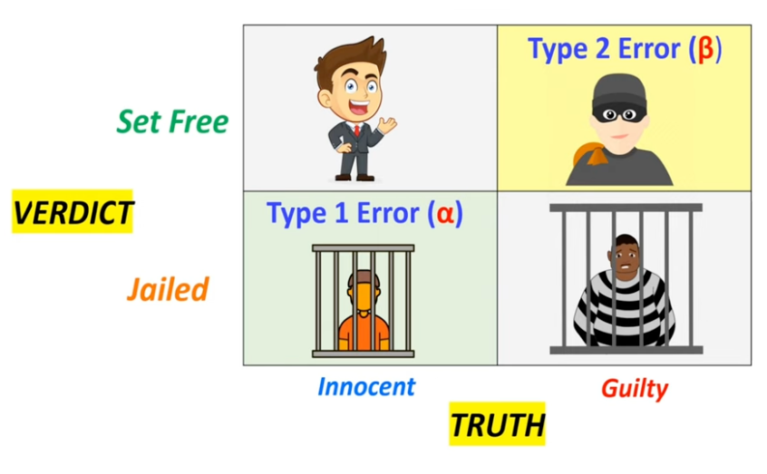
Null hypothesis (H0) is a statement that there is no relationship between two measured phenomena, or no association among groups. It is the default assumption that there is no effect or no difference. The alternative hypothesis (H1) is the statement that there is a relationship between two measured phenomena, or an association among groups. It is the opposite of the null hypothesis.
In the example of Innocent and Guilty, the null hypothesis is “Innocent” and the alternative hypothesis is “Guilty”. Type I error is the incorrect rejection of the null hypothesis (false positive), while Type II error is the failure to reject the null hypothesis when it is false (false negative).