Lesson Learned from NeurIPS 2023 Machine Unlearning Challenge
About the challenge
- Challenge page: https://www.kaggle.com/competitions/neurips-2023-machine-unlearning/overview, https://unlearning-challenge.github.io/
- Motivation of machine unlearning:
- Large models tend to memorize details of their training set and can be exploited to recover private information about individuals, i.e., by using membership inference attacks (Shokri et al., 2017) or model inversion attacks (Fredrikson et al., 2015).
- \(\rightarrow\) Privacy concerns arise when big tech companies collect and store large amounts of data about individuals (e.g., face images, voice recordings, search history, etc.) and train machine learning models on this data then release these models to the public, for example, StabilityAI’s Stable Diffusion models, Google’s Gemma, etc.
- \(\rightarrow\) Goverments and organizations (e.g., the European Union) have introduced regulations to protect individuals’ privacy rights (e.g., individuals have the “right to be forgotten” under the EU’s General Data Protection Regulation (Mantelero, 2013) or Canada’s Personal Information Protection and Electronic Documents Act)
- \(\rightarrow\) Machine learning developers like Google, OpenAI must ensure their models meet these requirements, i.e., they must be able to “unlearn” certain data from their models to comply with these regulations. These removal requests can be made by individuals or organizations and can be made at any time after the model has been trained and deployed.
- \(\rightarrow\) Retraining the model from scratch is very expensive and sometimes infeasible due to the entanglement of the data in the vast training set, for example, finding all Harry Potter references in a trillion tokens.
\(\rightarrow\) The need for machine unlearning algorithms that can remove specific data from a model without significantly affecting its performance on the remaining data


Task and Data
The challenge centers on the scenario in which an age predictor is built from face image data and, after training, a certain number of images must be forgotten to protect the privacy or rights of the individuals concerned.

Some teminologies/settings in the challenge (More details can be found in the challenge whitepaper)
- Original Model: A pre-trained model that predicts the age of a person from a face image. This is a discriminator/classifier model that takes an image as input and outputs a probability distribution over age classes.
- Train set \(D\): A set of face images with associated age labels used to train the model.
- Forget set \(S \subseteq D\): A set of face images with associated age labels that must be forgotten.
- Retain set: The set of face images with associated age labels that must be retained. This is the train set exclude the forget set \(D \ S\).
- Secret Model: The model that is trained on the retain set only. This is the model that the unlearning algorithm must produce/match.
- Goal: The unlearning algorithm must produce a model that is indistinguishable from the model trained without the forget set.
Define Machine Unlearning
For a fixed dataset \(D\), forget set \(S \subseteq D\), and a randomized learning algorithm \(A\), an unlearning algorithm \(U\) is \((\epsilon, \delta)\)-unlearning with respect to \((D, S, A)\) if for all regions \(R \subseteq \mathcal{R}\), we have that
\[Pr[A(D \setminus S) \in R] \leq e^{\epsilon} Pr[U(A(D),S,D) \in R] + \delta\]and
\[Pr[U(A(D),S,D) \in R] \leq e^{\epsilon} Pr[A(D \setminus S) \in R] + \delta\]where \(\mathcal{R}\) is the output space of the learning algorithm \(A\), for example, if using a neural network, \(\mathcal{R}\) is the space of all possible weight configurations of the network, and \(R\) is a region in this space.
\(A(D), A(D \setminus S)\) are the outputs of the learning algorithm \(A\) on the datasets \(D\) and \(D \setminus S\) (the “retain set”), respectively. \(U(A(D), S, D)\) is the output of the unlearning algorithm \(U\) on the model trained on \(D\), given access to the forget set \(S\) and the train set \(D\).
Intuitively, when \(\epsilon\) and \(\delta\) are small (i.e., \(e^{\epsilon} \approx 1 + \epsilon\) and \(\delta \approx 0\)), the unlearning algorithm \(U\) is indistinguishable from the learning algorithm \(A\) when the forget set \(S\) is removed from the train set \(D\).
Side note: The above definition is a bit different from the standard definition of differential privacy (DP). Please refer to the challenge whitepaper for more details.
Define the Evaluation Metric
The advantage of the above definition is that it is agnostic the output space of the learning algorithm \(A\) while not specifying the type of learning algorithm. This allows the definition to be applied to a wide range of learning algorithms, including discriminative models, generative models. However, this also makes it difficult to define a specific evaluation metric for the unlearning algorithm. For example, in the case of neural network, it is nearly impossible to compare the weights of the neural network before and after unlearning directly. In Differential Privacy literature, to evaluate the effectiveness of a DP algorithm, we make use of a membership inference attack, which can inspect the model output and determine whether a specific sample (i.e., \(S\)) was used in the training set or not. As defined above, the DP’s performance can be quantified by the \(\epsilon\) and \(\delta\) parameters, i.e., the smaller the \(\epsilon\) and \(\delta\), the better the DP algorithm.
DP can be interpreted as a hypothesis test with the null hypothesis that \(A\) was trained on \(D\) and the alternative hypothesis that A was trained on \(D \setminus S\). False positives (type-I errors) occur when the null hypothesis is true, but is rejected, while false negatives (type-II errors) occur when the alternative hypothesis is true, but is rejected. In Kairouz et al. (2015), the authors proposed an estimation of \(\epsilon\) at a fixed \(\delta\) as follows:
\[\hat{\epsilon} = \max \left\{ \log \frac{1 - \delta - \hat{\text{FPR}}}{\hat{\text{FNR}}}, \log \frac{1 - \delta - \hat{\text{FNR}}}{\hat{\text{FPR}}} \right\}\]where \(\hat{\text{FPR}}\) and \(\hat{\text{FNR}}\) are the false positive rate and false negative rate of the membership inference attack, respectively. The FPR and FNR can be estimated by repeating unlearning and retraining, then testing whether their outputs can be distinguished for each fixed forget example \(s=(x,y)\). In the unlearning test, the two hypotheses are unlearned versus retrained without the forget set. Let \(t_i^U=h(U_i(x))\) and \(t_i^R=h(R_i(x))\) be the scalar outputs from \(N\) runs of each procedure. The released evaluator uses \(h(M(x))=\log[p_M(y\mid x)/(1-p_M(y\mid x))]\), with numerical stabilization. For a decision rule \(g\), choose the convention \(g(t)=1\) meaning “retrained.” Then
The evaluator searches single- and double-threshold rules and retains the largest estimated \(\epsilon_s\) among the tested attacks, using \(\delta=10^{-5}\). The implementation can reverse which distribution receives the positive label; exchanging the two labels exchanges FPR and FNR without changing the symmetric \(\hat\epsilon\) formula above. These error rates are estimated across model runs for one fixed example, then per-example forgetting scores are aggregated. They are not obtained by mixing different forget examples into one confusion matrix. The competition used 512 unlearning runs from the same original checkpoint and 512 retrained models. Small estimated errors indicate distinguishability; large errors under the tested attacks remain empirical evidence rather than a certified guarantee. Official metric implementation, organizer protocol
The final evaluation metric as follow:
\[\mathcal{F}(\hat{\epsilon}) \times \frac{\text{RA}^{U}}{\text{RA}^{R}} \times \frac{\text{TA}^{U}}{\text{TA}^{R}}\]where \(\mathcal{F}(\hat{\epsilon})\) is a function of \(\hat{\epsilon}\) that rewards small values of \(\hat{\epsilon}\), \(\text{RA}, \text{TA}\) are the accuracy of the model on the retain set and holdout test set, respectively. The superscripts \(U, R\) denote the model produced by the unlearning algorithm and the secret model trained on the retain set, respectively. Intuitively, the above formula adjusts the forgetting quality F based on utility, by penalizing an unlearning algorithm if either its retain or test (average) accuracy is smaller than the corresponding average accuracy of retraining.
Winning solutions
Fanchuan is the winner on the final private leaderboard. The author’s write-up still has the title “2nd place solution”, while Kaggle identifies it as the first-place entry. These labels should not be confused with the public leaderboard used during development. The organizers explain that prizes used the final private leaderboard, obtained by evaluating submissions on a fresh dataset split. Their subsequent experiments used another split and a more extensive evaluation, so the ranking in those experiments is not the competition ranking. Official leaderboard, organizer report, Appendix A.3
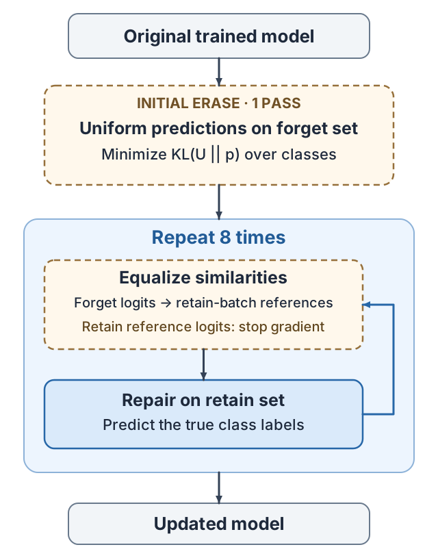
Fanchuan’s method starts with the trained model and changes its weights in two stages: one pass that makes predictions on forget examples more uniform, followed by eight cycles alternating a forget objective and ordinary supervised learning on the retain set. It is an example of erase and repair: deliberately disrupt the behavior associated with the forget set, then recover useful prediction behavior from retained data. The equations below follow the released notebook, including its loss signs and KL argument order.
First stage: weaken class-specific predictions on the forget set
Let \(z_\theta(x)\in\mathbb{R}^{C}\) be the classifier’s logits, \(p_\theta(x)=\operatorname{softmax}(z_\theta(x))\) its class probabilities, and \(u_c=1/C\) a uniform target over the \(C\) classes. Starting from the original parameters, the first stage minimizes
where \(B_F\) is a minibatch from the forget set. The ground-truth labels of these examples are not needed for this update. Instead, all classes receive equal target probability.
The direction of the gradient makes the mechanism concrete. For one example, the derivative with respect to logit \(z_c\) is \(p_c-1/C\). Gradient descent reduces logits whose probabilities exceed the uniform target and raises those below it. For a ten-class prediction with \(p_c=0.9\), that component contributes a positive gradient of \(0.8\); the update pushes its logit downward.
The notebook implements \(D_{\mathrm{KL}}(u\|p)\), because PyTorch receives log model probabilities as its first argument and uniform target probabilities as its second. This matters: \(D_{\mathrm{KL}}(p\|u)\) has the same uniform optimum but different gradients. The helper’s name, kl_loss_sym, also does not make the implemented loss symmetric. Winner’s notebook
Uniform predictions are an intermediate intervention, not the definition of successful unlearning. A model retrained without a particular face can still predict its age correctly from other faces. Making every forget example maximally uncertain could itself make the updated model distinguishable from retraining.
Second stage: alternate similarity equalization and retain training
The forget round draws a forget minibatch \(B_F\) and a retain minibatch \(B_R\). It computes the two sets of logits with the same current model, then stops gradients through the retain logits. Write
where \(\operatorname{sg}\) means stop-gradient and the notebook uses \(\tau=1.15\). For each forget example, \(q_{i,:}\) is a distribution over the retain examples in that minibatch, not over age classes. The implemented loss is
This is uniform-target cross-entropy over a row of similarities. Its gradient with respect to \(a_{ij}\) is \((q_{ij}-1/\lvert B_R\rvert)/\lvert B_F\rvert\). The update therefore reduces unusually strong associations and raises unusually weak ones. At the optimum, each retain example receives equal probability within that row.
That interpretation is more precise than saying “push forget examples away from everything.” Softmax is unchanged if the same constant is added to every similarity in a row, so this loss does not directly constrain their common absolute value. Nor does it select a positive pair as standard contrastive learning would. The code uses raw output logits, with no cosine normalization or separate feature encoder. Stopping the retain branch prevents this loss from backpropagating through those reference computations; the shared model’s parameters still change through the forget branch. Winner’s implementation
The retain round then makes a full pass over the retained examples using their true labels:
This repairs accuracy affected by the preceding forget round. Repeating the pair of operations lets the method revisit the forgetting objective after retained-data learning changes the same weights. There is no retrained oracle inside the algorithm: the secret model is used by the evaluator, not as a training target.
Pseudocode and implementation details
The following pseudocode preserves the objective and update order. It omits device transfers, logging, and checkpoint packaging; loaders are shuffled, and batches contain images and age-group labels as in the challenge notebook.
import torch
import torch.nn.functional as F

def fanchuan_unlearn(model, forget_loader, retain_loader):
    # Rebuild retain loaders with batch size 256 and independent shuffling.
    retain_train = shuffled_loader(retain_loader.dataset, batch_size=256)
    retain_refs = shuffled_loader(retain_loader.dataset, batch_size=256)

    # Separate optimizer objects retain separate momentum histories.
    initial_opt = torch.optim.SGD(model.parameters(), lr=0.005, momentum=0.9)
    forget_opt = torch.optim.SGD(model.parameters(), lr=3e-4, momentum=0.9)
    retain_opt = torch.optim.SGD(
        model.parameters(), lr=0.004, momentum=0.9, weight_decay=0.01
    )
    schedule = torch.optim.lr_scheduler.CosineAnnealingLR(
        forget_opt, T_max=8 * len(forget_loader), eta_min=1e-6
    )

    def update(optimizer, loss):
        optimizer.zero_grad()
        loss.backward()
        optimizer.step()

    model.train()
    for batch in forget_loader:  # Initial stage: one pass.
        logits = model(batch["image"])
        uniform = torch.full_like(logits, 1 / logits.shape[-1])
        loss = F.kl_div(F.log_softmax(logits, dim=-1),
                        uniform, reduction="batchmean")
        update(initial_opt, loss)

    for _ in range(8):
        # zip follows the released code: stop when either loader ends.
        for forgotten, retained in zip(forget_loader, retain_refs):
            z_forget = model(forgotten["image"])
            z_retain = model(retained["image"]).detach()
            similarities = z_forget @ z_retain.T / 1.15
            loss = -F.log_softmax(similarities, dim=-1).mean()
            update(forget_opt, loss)
            schedule.step()

        for retained in retain_train:
            logits = model(retained["image"])
            loss = F.cross_entropy(logits, retained["age_group"])
            update(retain_opt, loss)
    return model
All three SGD optimizers use momentum \(0.9\). The initial and similarity stages have zero weight decay; the retain stage uses \(0.01\). Its learning rate is \(0.001\times256/64=0.004\) in the released recipe. The cosine schedule advances after each similarity update, not after each retain epoch. Keeping separate optimizers also keeps their momentum buffers separate; merging the losses into one optimizer would change the recipe. These are competition settings rather than universal defaults. Released code
The author’s write-up reports that adding cosine annealing to forget rounds improved the public score from \(0.084\) to \(0.091\). This is a development observation, not an isolated, repeated ablation or the final winning score. The larger retain batch enabled eight repair epochs within the available runtime. The competition required producing 512 unlearned checkpoints within eight hours, so runtime constrained how much repair could be performed. Author’s write-up, competition setup
What the other leading solutions and later evaluation teach us
The organizers’ June 2024 retrospective, published after this post’s original date, places Fanchuan alongside other leading methods. They share the erase/repair pattern but implement it differently:
| Entry | Erase operation | Repair operation |
|---|---|---|
| Fanchuan | Uniform class targets, then equalized forget-to-retain similarities | Cross-entropy on retain labels between forget rounds |
| Kookmin | Reinitialize convolutional parameters with the lowest 30% gradient magnitudes under its selection objective | Retain training, with smaller gradient multipliers for unchanged parameters |
| Seif | Perturb convolutional weights with Gaussian noise | Retain training with a batch-dependent weighting rule |
| Sebastian | Replace 99% of convolutional/linear weights selected by small magnitude | Retain cross-entropy plus a penalty matching the original model’s prediction entropy |
These are distinct submissions; weight reinitialization, parameter noise, and entropy matching should not be attributed to Fanchuan. Organizer method descriptions
The retrospective’s comparison separates forgetting quality from the utility-adjusted score. It shows why a strong forgetting score can coexist with substantial loss of useful behavior.


Sebastian achieved the strongest forgetting score in that experiment but paid a larger utility penalty after replacing most weights. Fanchuan was more sensitive to whether repeated unlearning runs started from one original checkpoint or different independently trained checkpoints. The cheaper single-checkpoint setup used during the competition underestimated its forgetting score in the report’s comparison. On FEMNIST, transferring the same hyperparameters or only lightly tuning them did not preserve all of the competition methods’ advantages. These observations support evaluating utility, initialization sensitivity, and transfer separately rather than treating a single rank as a universal recommendation. Retrospective experiments
A winning score is empirical evidence, not a deletion certificate
The evaluator compares distributions of a scalar statistic—the log-odds of the correct-class probability—across unlearned and retrained models, separately for each forget example. It searches single- and double-threshold attacks, estimates an \(\epsilon\) from their errors, then aggregates scores across examples. This is stronger evidence than simply checking that forget-set accuracy fell: matching the retrained model’s accuracy can still leave distinguishable confidence distributions. Official evaluation code
The formal definition earlier in this post quantifies over all measurable regions of model outputs. A finite collection of attacks on one scalar statistic cannot establish that requirement. Small empirical \(\hat\epsilon\) values mean those tested attacks failed to distinguish the sampled distributions strongly; they do not supply a certified upper bound on every possible attack. Finite samples, threshold selection, averaging across easy and difficult forget examples, and the chosen data split all affect the result. Fanchuan’s contribution is a concrete, efficient recipe that performed well under the challenge’s empirical protocol. Its success motivates careful reuse and further evaluation, rather than a claim that every trace of a subject has been provably removed. Evaluation framework and limitations
References
Enjoy Reading This Article?
Here are some more articles you might like to read next: