Kolmogorov-Arnold Network (KAN)
Resources:
- [1] KAN Paper
- [2] KAN Github
- [3] Awesome KAN(Kolmogorov-Arnold Network)
- [4] Philosophical thoughts on Kolmogorov-Arnold Networks by Ziming Liu
- [5] Kolmogorov-Arnold Networks (KAN) Promising Alternative to Multi-Layer Perceptron? by DigitalOcean
- [6] KAN or MLP: A Fairer Comparison
MLP vs KAN

Limitations of MLP:
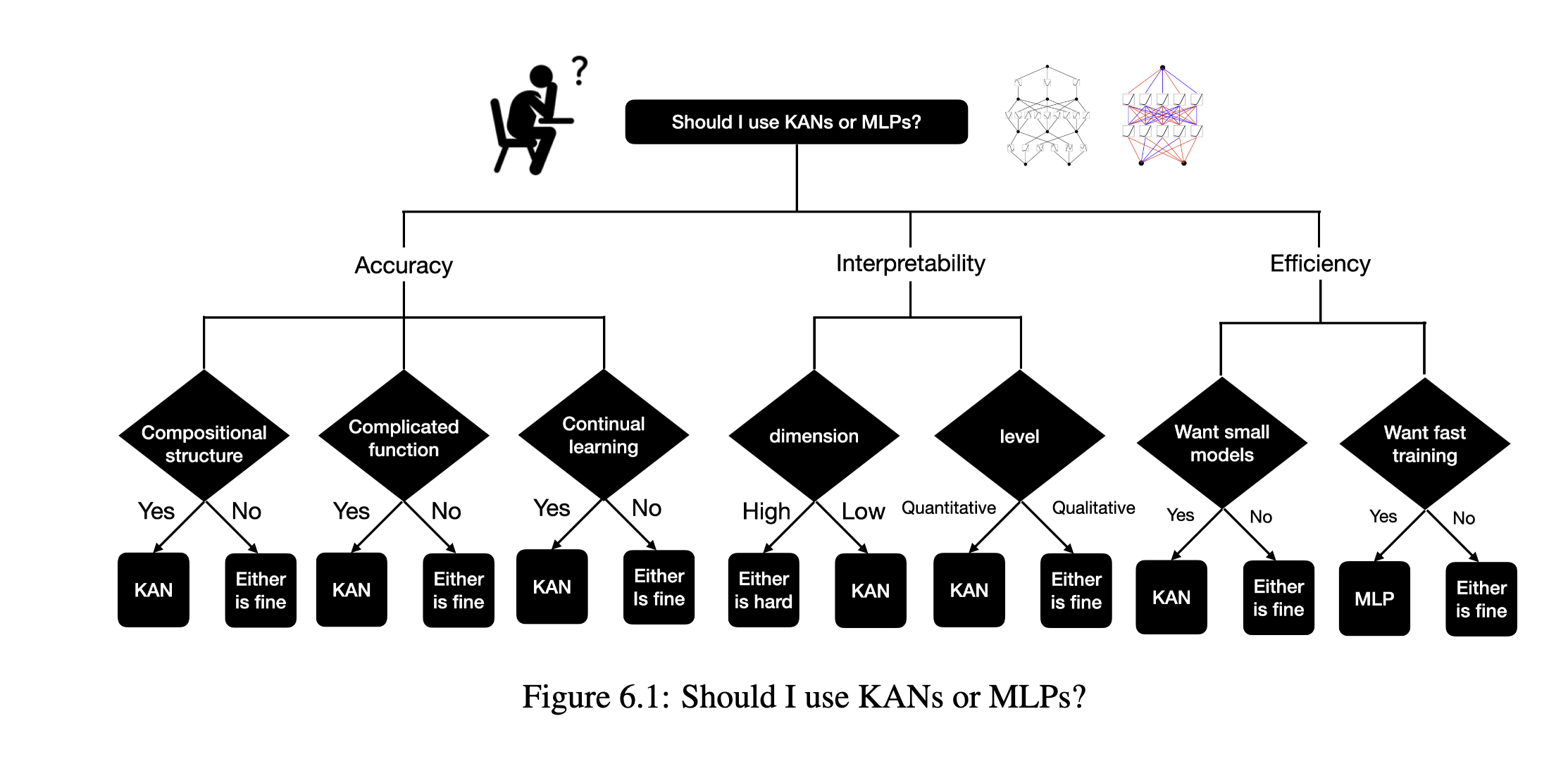
- Interpretability: MLPs are often considered “black boxes” due to their complex internal workings, making it difficult to understand how they arrive at their predictions.
- Curse of Dimensionality: MLPs can struggle with high-dimensional data, as the number of parameters required to capture complex relationships grows exponentially with the input dimension.
- Local Optimization: MLPs rely on gradient-based optimization algorithms, which can get stuck in local minima, potentially leading to suboptimal solutions.
- Catastrophic Forgetting: MLPs can be prone to catastrophic forgetting, where learning new information can overwrite previously learned knowledge, hindering their ability to perform continual learning.
Advantages of KAN over MLP:
- Interpretability: KANs are more interpretable than MLPs due to their structure and the use of learnable activation functions. The absence of linear weight matrices and the explicit representation of univariate functions make it easier to understand how KANs arrive at their predictions.
- Neural Scaling Laws: KANs exhibit faster neural scaling laws than MLPs, meaning that their performance improves more rapidly with increasing model size. This faster scaling can lead to significant gains in accuracy by simply scaling up the model.
- Continual Learning: KANs can naturally perform continual learning without catastrophic forgetting, unlike MLPs. This ability stems from the locality of spline basis functions, which allows KANs to update knowledge in specific regions without affecting previously learned information.
Limitations of KAN:
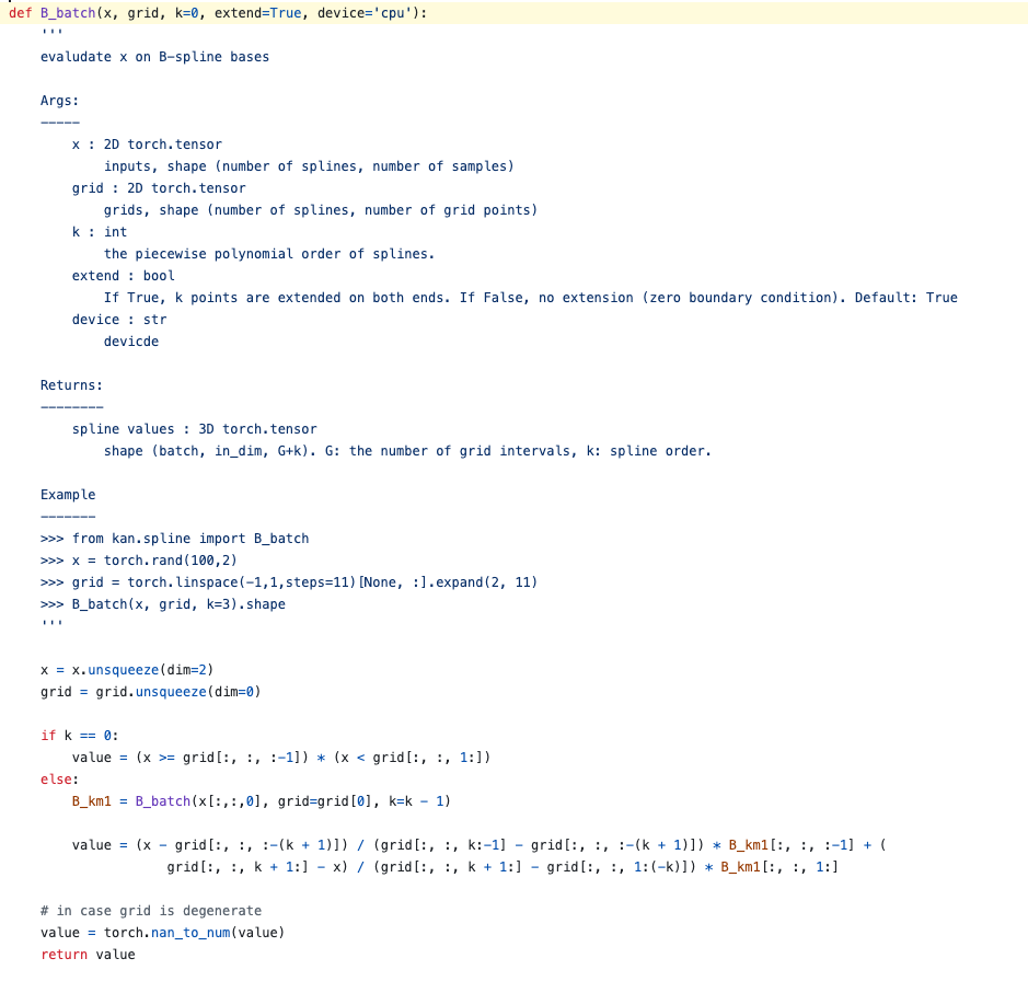
- Computational Efficiency: KANs can be computationally more expensive to train than MLPs due to the complexity of learning and evaluating spline functions. The current implementation of this spline function can be found here, which requires recursive computation of a higher-order spline from lower-order splines. This process does not leverage the parallelization of modern GPUs.
- Theoretical Limitations: The Kolmogorov-Arnold Representation Theorem (KAT) primarily applies to single layer KANs, and therefore the multi-layer KANs are not guaranteed to be able to represent any continuous function. For example, the input of the activation function should be bounded, which is not trivial for multi-layer KANs.

KAN or MLP: A Fairer Comparison
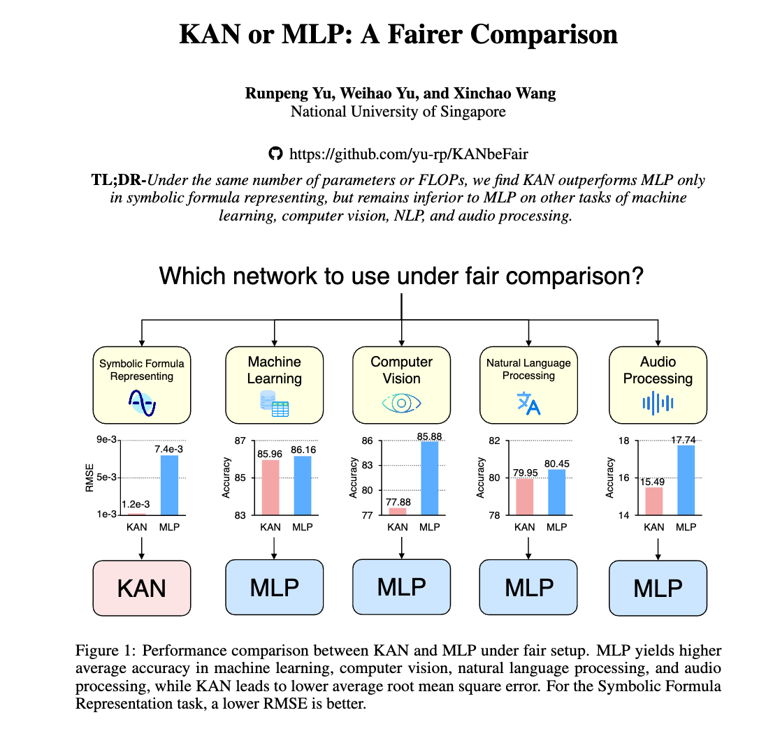
Paper [6] provides a fairer comparison between KAN and MLP by considering the same number of parameters and FLOPs to make sure that the computational complexity is the same. The tasks for comparison are also more comprehensive, including tasks in ML, CV, NLP and symbolic formula representation.

The key findings are follows, which somewhat contradict to the observation in the original KAN paper [1].
- Symbolic Formula Representation: KANs outperform MLPs when approximating symbolic formulas.
- Other Tasks: MLPs generally outperform KANs on other tasks, including machine learning, computer vision, natural language processing, and audio processing.
- Impact of B-spline Activation: KANs’ advantage in symbolic formula representation comes from their use of B-spline activation functions. When MLPs use B-spline activation functions, their performance on symbolic formula representation matches or exceeds that of KANs. However, B-spline activation functions do not significantly improve MLPs’ performance on other tasks.
- Continual Learning: KANs do not outperform MLPs in continual learning tasks. In a standard class-incremental continual learning setting, KANs forget old tasks more quickly than MLPs.
KAN
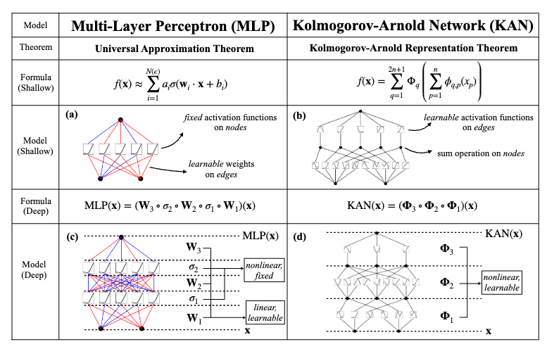
Before we dive into the KAN, let’s first understand the two definitions “edge” and “node” in MLP and KAN. Given a MLP with \(n\) input nodes and \(m\) output nodes, the MLP can be represented as a directed acyclic graph (DAG) as follows:

Mathematically, the node \(y_i\) of the output (hidden) layer can be represented as \(y_i = \sigma \left( \sum_{j=1}^{n} w_{i,j} x_j\right)\) where \(x_j\) is the input node, \(w_{i,j}\) is the weight. We ignore the bias term for simplicity. The connection between the input nodes \(x_j\) and the output node \(y_i\) is called an edge, which is scaled by the learnable weight \(w_{i,j}\). After applying the sum operation over all the edges, the output node \(y_i = \sigma \left( \sum_{j=1}^{n} w_{i,j} x_j \right)\) is obtained by applying the non-linear activation function \(\sigma\) on the weighted sum. Note that the activation function \(\sigma\) is pointwise applied and not learnable.
For the Kolmogorov-Arnold Network (KAN), it is based on the Kolmogorov-Arnold Representation Theorem (KAT). KAT states that any continuous function can be represented as a sum of a trigonometric polynomial and a spline function. More specifically, the multivariate continuous function \(f: [0,1]^n \rightarrow \mathbb{R}\) can be represented as:
\[f(x) = f(x_1, x_2, \cdots, x_n) = \sum_{q=0}^{2n+1} \Phi_q \left( \sum_{p=1}^{n} \phi_{q,p}(x_p) \right)\]where \(\phi_{q,}:[0,1] \rightarrow \mathbb{R}\) are the learnable activation functions over edges, and the \(\Phi_q\) is the learnable activation function over output nodes.
In KAN, the edge connection between the input nodes \(x_p\) and the output node \(y_q\) is applied by the learnable activation function \(\phi_{q,p}\). After applying the sum operation over all the edges, the output node \(y_q = \Phi_q \left( \sum_{p=1}^{n} \phi_{q,p}(x_p) \right)\) is obtained by applying another learnable activation function \(\Phi_q\).

So compared to MLP, while the process from input nodes to output nodes is quite similar (one output node connected to all the input nodes), and the activation function on edges \(\phi_{q,p}\) is also parameterized similar to \(w_{i,j}\) in MLP, the main difference lies in the activation function on output nodes \(\Phi_q\) that is learnable in KAN.
Implementation of KAN
Residual Activation Function
Beside the spline function, the activation function also includes a basis function \(b(x)\) which gets the signal directly from the input nodes (without going through any weight matrix).
\[\phi(x) = w_b b(x) + w_s \text{spline}(x)\]where \(w_b\) and \(w_s\) are the learnable weights. the basis function \(b(x) = \text{silu}(x) = x / (1 + e^{-x})\).
The most complicated part is the spline function, which is parameterized as a linear combination of B-splines such as:
\[\text{spline}(x) = \sum_{i=1} c_i B_i(x)\]where \(B_i(x)\) is the \(i\)-th B-spline and \(c_i\) is the learnablecoefficient.
B-spline
B-splines are essentially curves made up of polynomial segments, each with a specified level of smoothness. Picture each segment as a small curve, where multiple control points influence the shape. Unlike simpler spline curves, which rely on only two control points per segment, B-splines use more, leading to smoother and more adaptable curves.
The magic of B-splines lies in their local impact. Adjusting one control point affects only the nearby section of the curve, leaving the rest undisturbed. This property offers remarkable advantages, especially in maintaining smoothness and facilitating differentiability, which is crucial for effective backpropagation during training (From [4]).

Mathematically, B-splines can be constructed by means of the Cox-de Boor recursion formula (Wikipedia), starting with the B-spline basis function of order 0. We start with the B-splines of degree \(p = 0\), i.e. piecewise constant polynomials:
\[B_{i,0}(t) := \begin{cases} 1 & \text{if } t_i \leq t < t_{i+1}, \\ 0 & \text{otherwise.} \end{cases}\]The higher \((p + 1)\)-degree B-splines are defined by recursion:
\[B_{i,p}(t) := \frac{t - t_i}{t_{i+p} - t_i} B_{i,p-1}(t) + \frac{t_{i+p+1} - t}{t_{i+p+1} - t_{i+1}} B_{i+1,p-1}(t).\]The implementation of the B-spline can be found here.

Computational Expensiveness: Because of the recursive computation of the B-spline, the computational complexity is much higher than that of MLP.
Grid Extension
The grid extension in KAN is the process of refining the spline function by adding more knots, so that the spline function can have a higher resolution, fit the data better. It can be done by using higher-order B-splines, which is calculated by the lower-order B-splines (therefore, it is called extension).
Philosophical thoughts on KAN by Kan’s author
I found the philosophical thoughts on KAN by the author here very interesting and helpful to understand the KAN and its difference with MLP. I just quote the part that I think is most relevant to the KAN here.
Reductionism vs. Holism While MLPs are more aligned with holism, KANs are more aligned with reductionism. The design principle of MLPs is “more is different”. In an MLP, each neuron is simple because it has fixed activation functions. However, what matters is the complicated connection patterns among neurons. The magical power of MLPs performing a task is an emergent behavior which is attributed to collective contribution from all neurons. By contrast, in a KAN, each activation function is complicated because it has learnable functions. By sparsification and pruning, we hope the computation graph to be simple. In summary, MLPs have simple ‘atoms’ but complicated ways to combine these atoms; KANs have complicated (diverse) ‘atoms’ but simple ways to combine these atoms. In this sense, MLPs’ expressive power comes from the complicated connection patterns (fully-connected structure), which give rise to emergent bahavior (holism). In contrast, KANs’ expressive power comes from the complexity of fundamental units (learnable activation functions), but the way to decompose whole network to units is simple (reductionsim)
Attention Mechanism
Because of the spline function \(\text{spline}(x)\), which is a linear combination of B-splines with different level of smoothness/resolution of the input \(x\), each resolution is weighted by the learnable coefficient \(c_i\), this mechanism can be regarded as a soft self attention mechanism, where the output attends to different parts of the input with different resolutions.
Enjoy Reading This Article?
Here are some more articles you might like to read next: