Stanford CS231N | Spring 2025 | Lecture 2- Image Classification with Linear Classifiers
- Course session overview: image classification and path toward neural networks
- Syllabus context and immediate lecture goals
- Definition of the image classification task
- Images as numerical tensors and basic image representation
- Semantic gap and sensitivity to viewpoint changes
- Illumination effects on pixel values
- Additional imaging challenges: background, scale, resolution, occlusion, deformation, intraclass variation and context
- Limitations of hand-crafted rule-based recognition pipelines
- Datadriven three-step procedure for supervised classification
- Overview of two exemplar datadriven classifiers: nearest neighbor and linear classifiers
- K-nearest neighbor training and prediction conceptual overview
- Distance functions for nearest neighbor and L1 definition
- Practical implementation notes: vectorized distance computation
- Image storage formats and pixel quantization rationale
- Computational complexity of k-NN: O(1) training and O(n) prediction
- Geometric visualization of one-nearest-neighbor partitions (Voronoi regions)
- Robustness via k and tie/ambiguity regions as targets for data collection
- Manhattan (L1) versus Euclidean (L2) distance geometry
- Effect of distance metric on decision boundaries and feature representation
- Hyperparameters in k-NN and general model selection
- Validation, testing, and cross-validation for hyperparameter tuning
- Introduction to the CIFAR-10 dataset and k-NN qualitative results
- Empirical k selection on CIFAR-10 and baseline accuracy
- Failure modes of pixel-wise distances and translation sensitivity
- Transition to linear classifiers as parametric models
- Parameterization of linear classifiers: weight matrix and bias
- Linear models as foundational components of neural networks
- Simplified 2×2 image example to illustrate linear scoring
- Visual templates and geometric decision boundaries for linear classifiers
- Limitations of linear separability
- Role of a loss function and optimization objective
- Softmax transformation: converting logits to class probabilities
- Negative log-likelihood (softmax loss) and relation to logistic regression
- Information-theoretic interpretations: KL divergence and cross-entropy
Course session overview: image classification and path toward neural networks

This lecture focuses on image classification and places the material on a clear path toward neural and convolutional neural network methods.
It begins with linear classifiers and will later connect these building blocks to deeper architectures.
- The pedagogical arc moves from basic data-driven methods toward components used in modern deep learning.
- The lecture sets expectations for algorithmic and conceptual foundations that will be extended in later sessions.
Framing note: linear classifiers are presented as an early building block that will be expanded into more complex models in subsequent lectures. The content builds on the previous session and covers foundations relevant to CS231N.
Syllabus context and immediate lecture goals
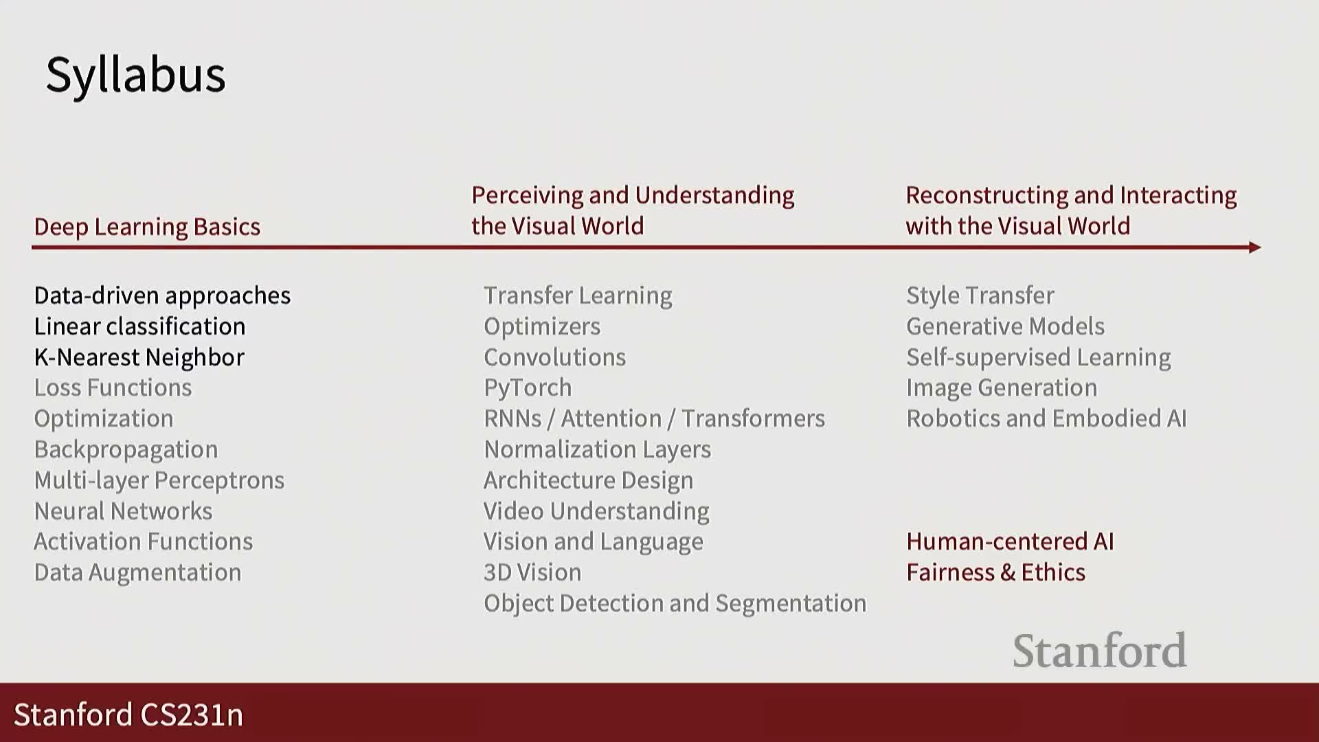
This section places the lecture in the course syllabus and clarifies immediate learning objectives.
- Core aims today: data-driven approaches, linear classification, and k-nearest-neighbor (k-NN) methods.
- Course-wide themes enumerated:
-
Deep learning basics
-
Perceiving and understanding the visual world
-
Reconstructing and interacting with the visual world
-
Deep learning basics
Context: image classification recurs across the quarter as a core benchmark task. Today’s goals emphasize comparing simple nonparametric approaches with parametric linear models to build intuition for later deep-learning topics.
Definition of the image classification task
Image classification: assign one label from a predefined vocabulary to an input image.
- Labels come from a fixed set (e.g., dog, cat, truck, plane) and are selected for each input image.
- Humans perform this mapping effortlessly, but converting raw pixel data into semantic labels is a nontrivial algorithmic problem.
Why it matters: this canonical task motivates the development of systematic algorithms and benchmark evaluations, and it provides repeatable examples to illustrate algorithmic behavior across the course.
Images as numerical tensors and basic image representation

Images are formalized as numerical arrays—specifically tensors with height, width, and channel dimensions.
- Colored images are typically represented as H × W × 3 tensors for RGB images.
- Typical pixel values are integers in the 0–255 range for 8-bit channels; an example resolution might be 32 × 32 × 3 to illustrate dimensionality.
Implication: representing images as raw numbers exposes a semantic gap between human perception and machine input, motivating the need for features or learned mappings to bridge that gap. The simplicity of storing pixels belies the recognition challenges that follow.
Semantic gap and sensitivity to viewpoint changes
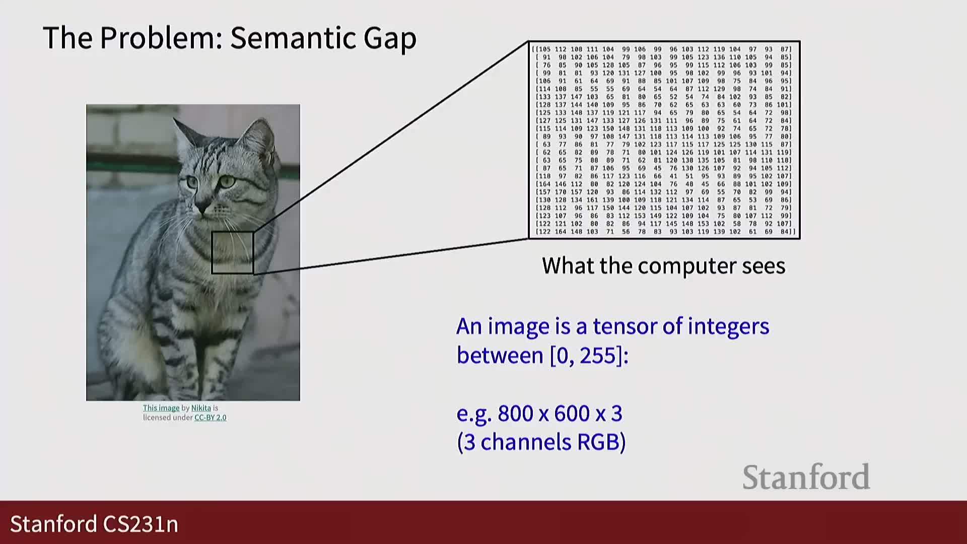
There is a large semantic gap between human perception and raw pixel data; camera motion illustrates this clearly.
- Small viewpoint changes (pan/shift) can produce completely different pixel arrays for the same object.
- Even tiny translations alter many or all pixel values in a high-dimensional image tensor, so naive pixel matching fails to capture object identity invariances.
Conclusion: viewpoint variation is a fundamental source of variability that recognition systems must handle via feature design or learning to achieve geometric robustness.
Illumination effects on pixel values
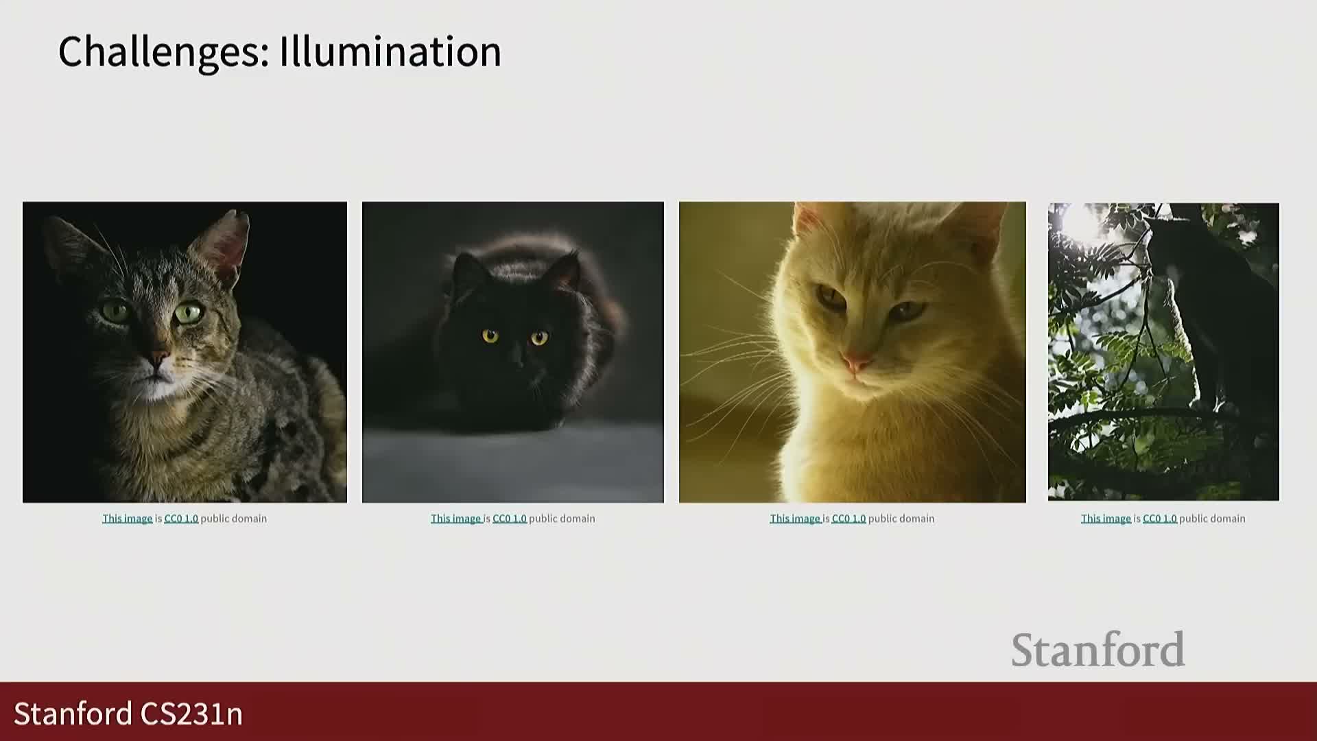
Illumination variation is a major challenge in image recognition.
- Observed RGB values depend on surface reflectance, material properties, and lighting conditions.
- The same object photographed under different lighting can yield drastically different pixel values despite unchanged semantic labels.
This variability motivates the use of invariant features, normalization, data augmentation, and learned models that reduce sensitivity to lighting changes.
Additional imaging challenges: background, scale, resolution, occlusion, deformation, intraclass variation and context
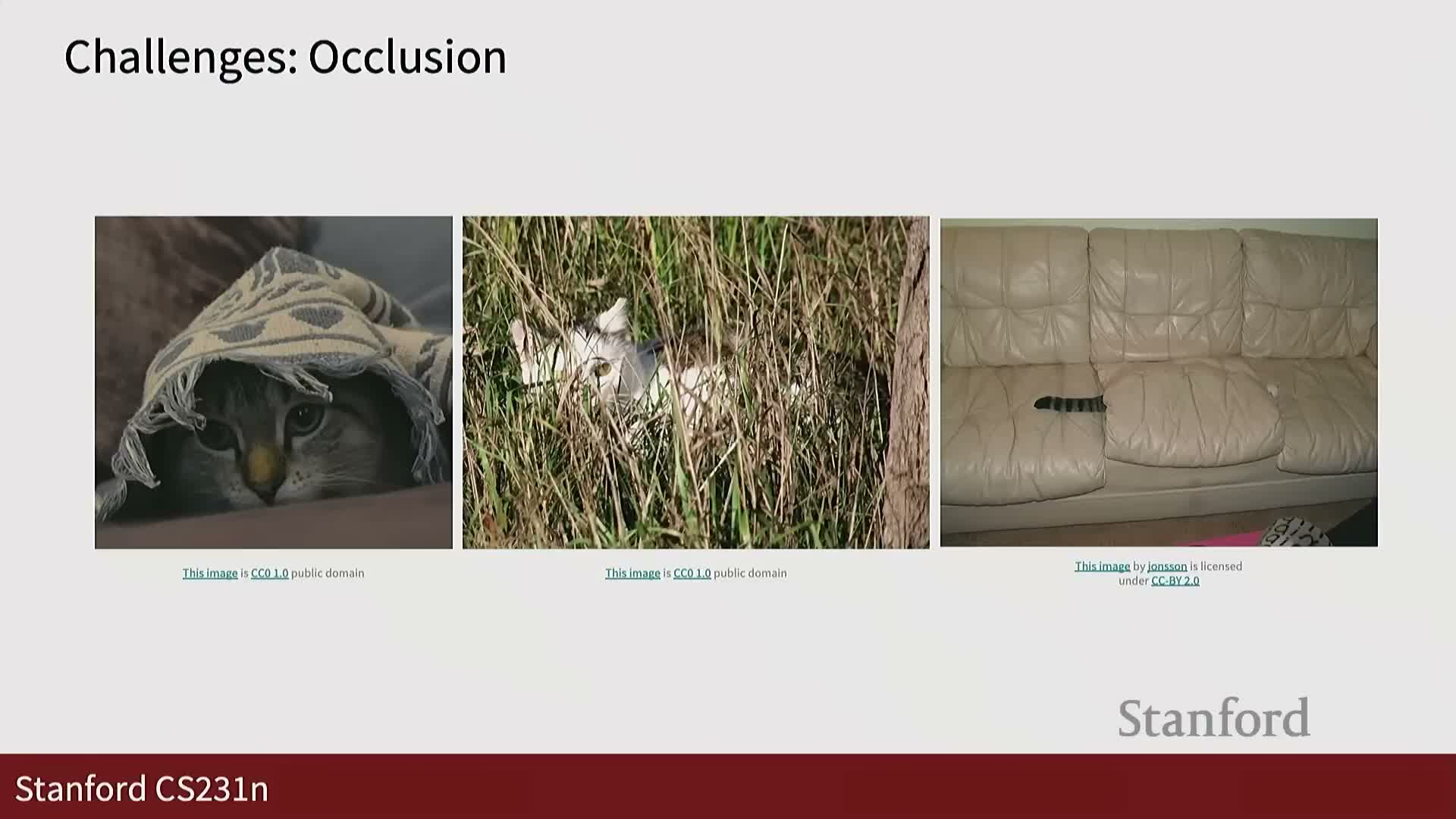
Recognition challenges are broad and numerous. Key factors include:
-
Background clutter that confuses object boundaries
-
Scale changes (zoom) and varying resolution
-
Occlusion and severe partial visibility
-
Object deformation and wide intra-class variation (size, color, breed)
- The importance of contextual cues (e.g., living room vs. street) for disambiguation
These factors change pixel values or visible object parts. Humans use context and prior knowledge to resolve ambiguities; machines must learn similar strategies, which is why learning-based approaches are preferred over brittle rule-based systems.
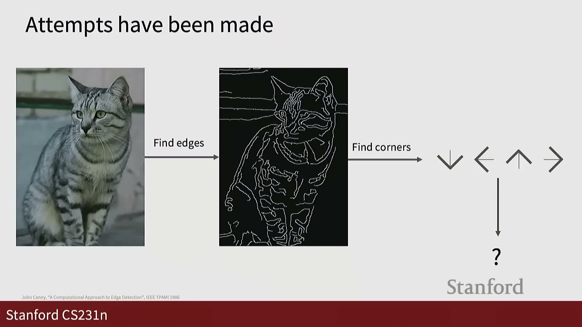
Limitations of hand-crafted rule-based recognition pipelines
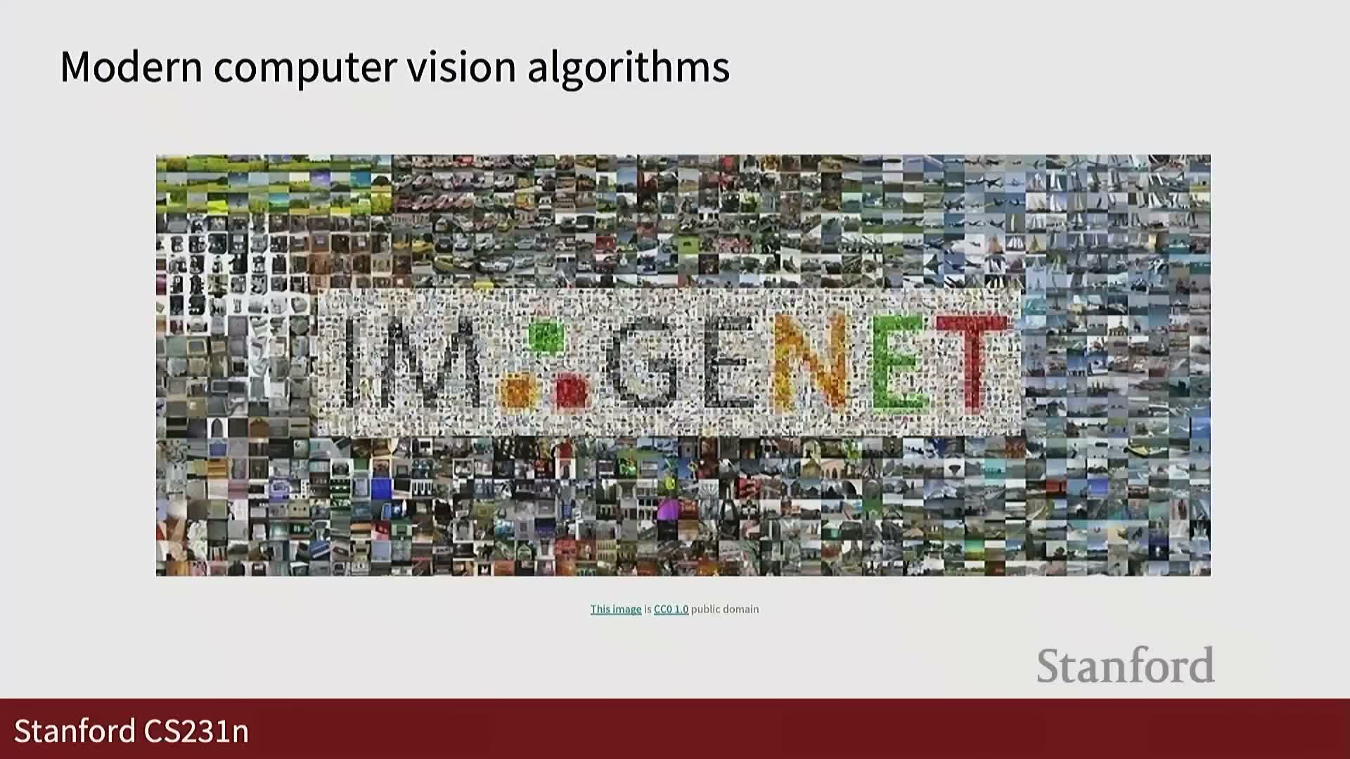
Historically, researchers handcrafted algorithms—edge detectors, corner statistics, and rule-based feature pipelines—to solve recognition tasks.
- Such explicit logic is labor-intensive and does not generalize well across object classes and varied imaging conditions.
- Designing rules for every class and scenario is hard to scale to large, natural image collections.
This motivates the shift to data-driven machine learning approaches that learn mappings from data rather than relying on manually engineered decision procedures.
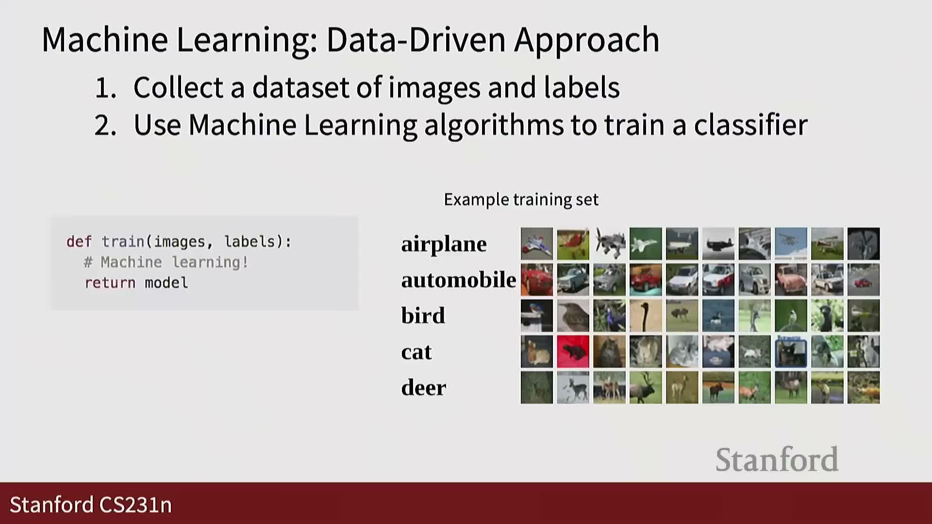
Datadriven three-step procedure for supervised classification
The standard data-driven pipeline for supervised image classification has three stages:
-
Collect labeled datasets that provide empirical examples.
-
Train a model that maps images to labels by fitting parameters to the labeled data.
-
Evaluate the trained model on held-out images using a prediction function to assess generalization.
Notes: datasets are the empirical basis for learning, training fits a parameterized function to associate inputs with labels, and evaluation measures performance on unseen data. Historical data-collection methods vary, but modern curated benchmarks are widely available and drive algorithmic choices.
Overview of two exemplar datadriven classifiers: nearest neighbor and linear classifiers
Two representative methods are introduced as pedagogical anchors:
-
Nearest neighbor (k-NN): a nonparametric, memory-based method that emphasizes distance metrics and design trade-offs.
-
Linear classifiers: parametric models with learned weights that introduce parameter estimation and optimization.
Role: k-NN builds intuition about similarity and hyperparameters, while linear models lay the groundwork for more complex neural architectures. Both are complementary educational examples.
K-nearest neighbor training and prediction conceptual overview

The k-nearest neighbor (k-NN) pattern is simple and transparent.
- The training function memorizes labeled examples—no parametric fitting occurs.
- The predict function computes a distance measure between a query and all stored training points, then assigns labels based on the most similar examples.
Strengths and limits: k-NN’s transparency is pedagogically useful, but the need to compare to all stored samples at test time makes it computationally expensive in practice.
Distance functions for nearest neighbor and L1 definition
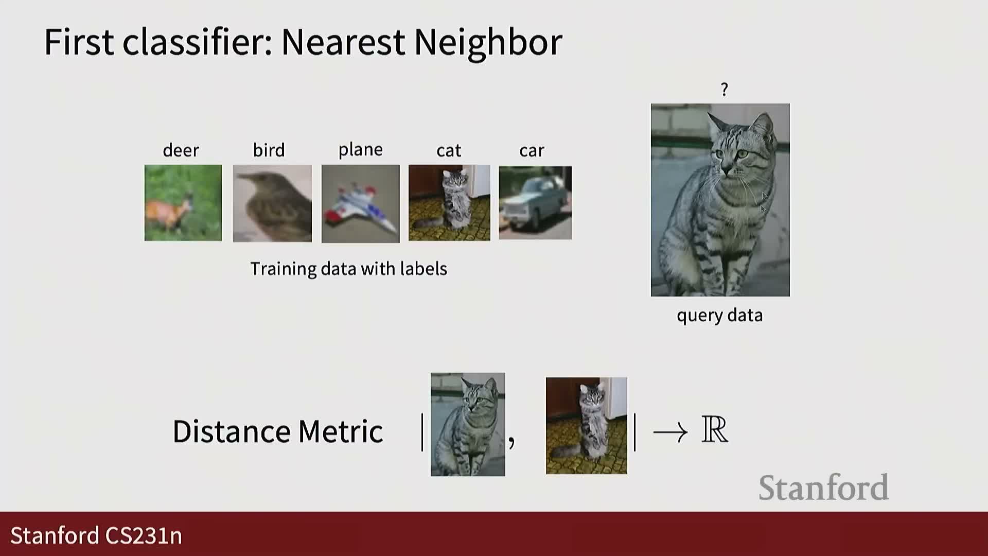
A distance function is central to k-NN. One common choice is the L1 distance (Manhattan distance).
-
L1 distance computes the sum of absolute pixel-wise differences between two images: element-wise absolute differences followed by summation across pixels and channels.
- L1 is simple, interpretable, and often effective—its choice strongly influences k-NN performance.
Choosing an appropriate distance metric is therefore critical for meaningful similarity comparisons.
Practical implementation notes: vectorized distance computation
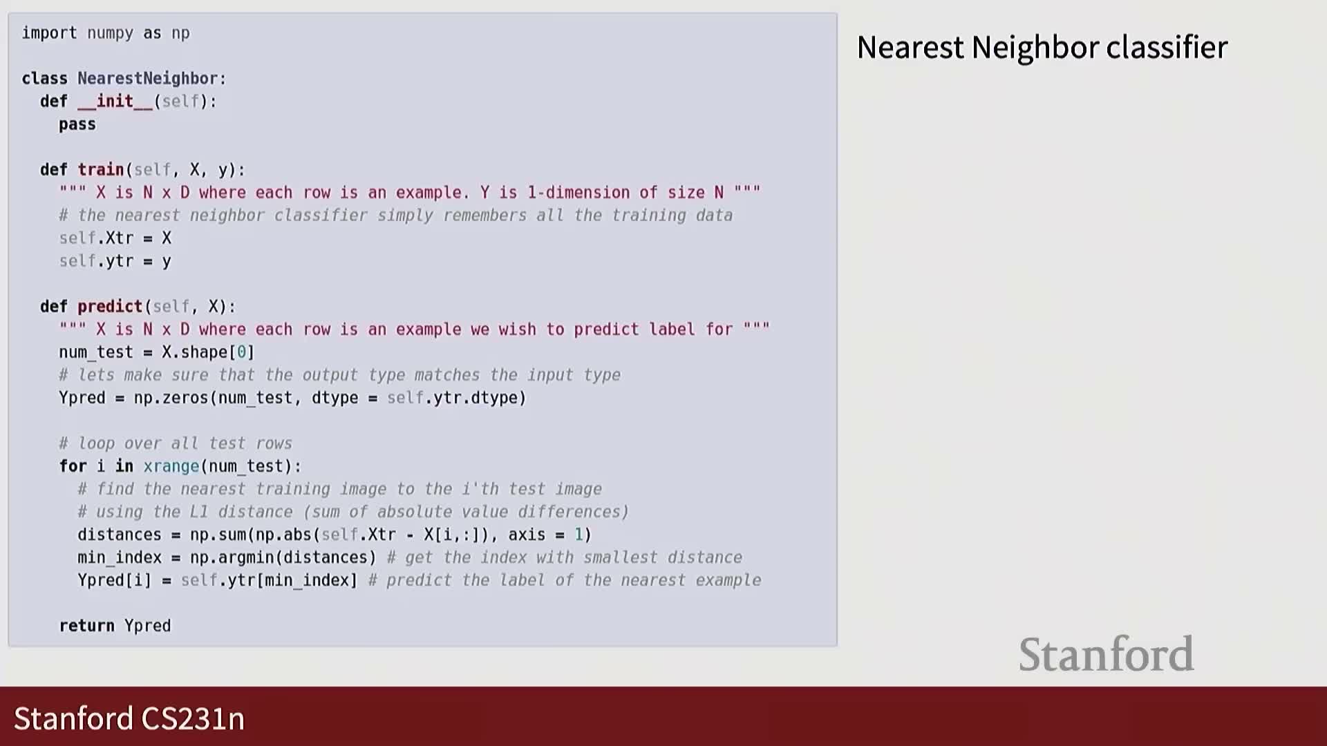
Practical k-NN prediction is implemented efficiently using vectorized numerical libraries (e.g., NumPy). Typical implementation steps:
-
Compute distances between each test sample and all training samples (vectorized pairwise computation).
-
Select the minimum (or k smallest) distances per test sample.
-
Return the corresponding training labels (e.g., via majority vote for k>1).
Notes: training is just memory storage. Efficient implementations leverage broadcasting and vectorized reductions to avoid Python loops, but prediction complexity still scales with the number of stored samples.
Image storage formats and pixel quantization rationale

Typical RGB pixel values range from 0–255 because of common 24-bit color image standards.
- Each color channel (R, G, B) uses 8 bits, yielding integer values in 0–255.
- Some formats add an alpha channel (occasionally 32-bit), but 24-bit RGB is the ubiquitous standard.
Practical implications: file format and quantization influence preprocessing decisions such as normalization and datatype conversion for machine learning pipelines.
Computational complexity of k-NN: O(1) training and O(n) prediction
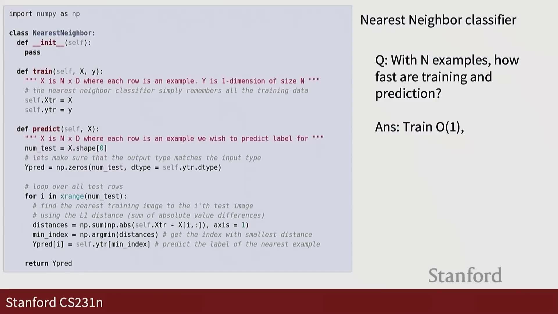
Algorithmic complexity analysis of k-NN (big-O notation):
-
Training time: O(1) per stored example—training merely stores the dataset.
-
Prediction time: O(n) per test sample, where n is the number of training examples, because distances to all stored examples must be computed.
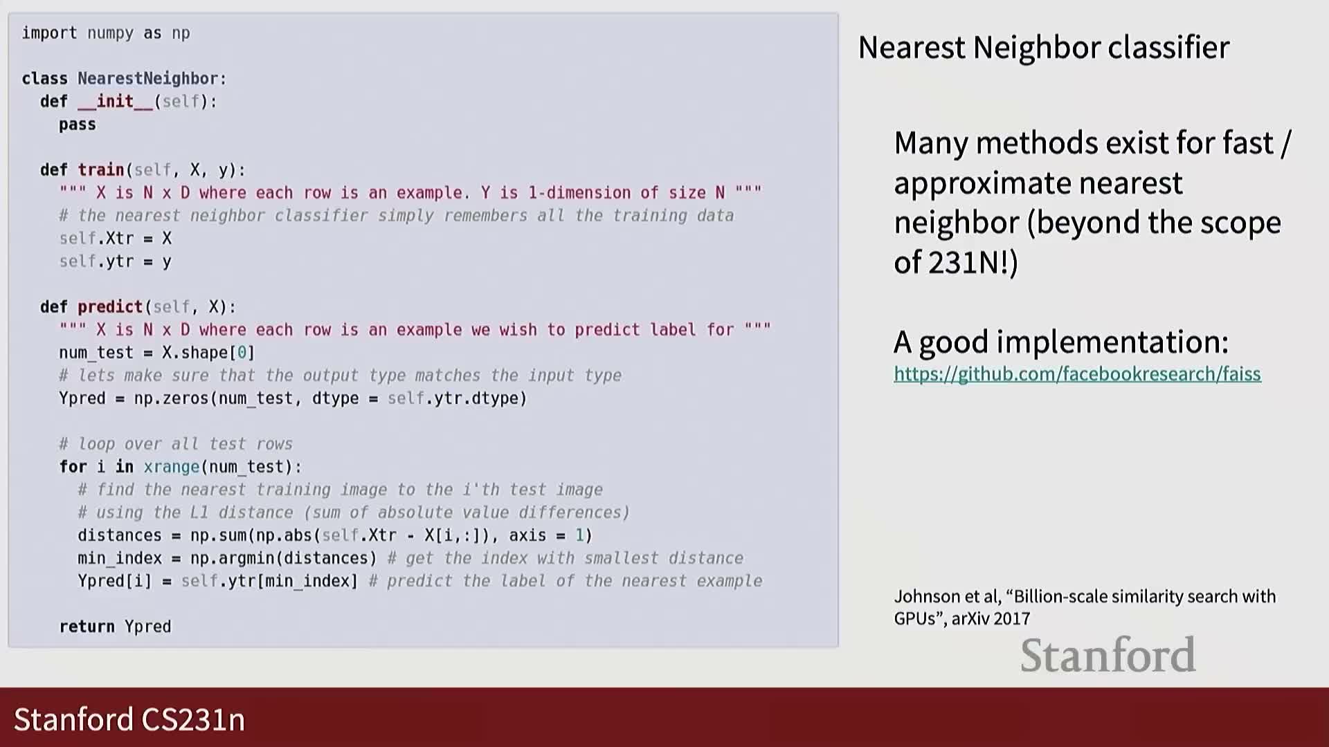
Consequence: exhaustive comparison at inference scales poorly for large datasets, motivating classifiers that trade higher offline training cost for faster online inference. Scalable k-NN variants exist but are beyond this lecture’s scope.
Geometric visualization of one-nearest-neighbor partitions (Voronoi regions)
A one-nearest-neighbor classifier partitions feature space into Voronoi cells.
- Each region is assigned the label of its nearest training point.
- Decision boundaries are determined by the loci of points equidistant to neighboring training samples.
Visualization intuition: sparse or noisy training points create anomalous regions, which highlights robustness issues and the discrete sample-driven nature of k-NN boundaries.
Robustness via k and tie/ambiguity regions as targets for data collection
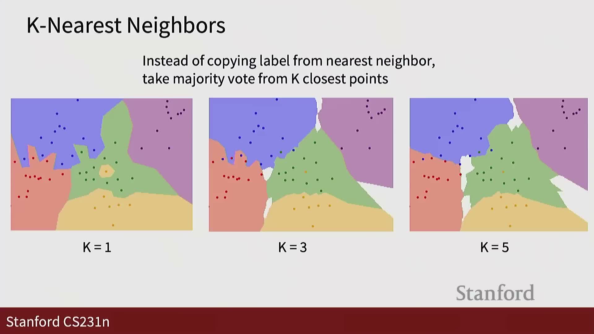
Increasing k introduces voting and reduces sensitivity to individual noisy samples.
- With k>1, labels are assigned by majority vote among nearest neighbors, which mitigates outlier-induced misclassification.
- However, larger k can create ambiguous regions where votes tie or remain inconclusive—these reveal areas where additional data would be most helpful.
Practical takeaway: k-NN with k>1 smooths decisions but highlights local uncertainty useful for targeted data collection.
Manhattan (L1) versus Euclidean (L2) distance geometry
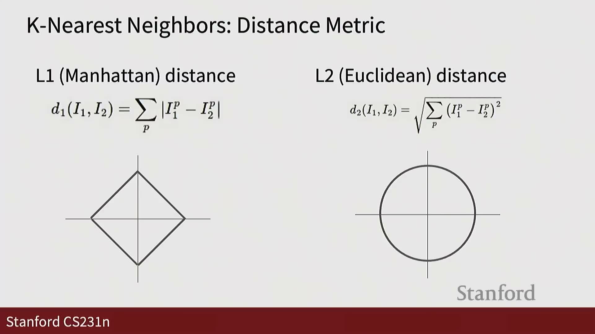
Geometric comparison of L1 and L2 distances:
-
L1 contours (equidistance) form axis-aligned diamond/square shapes.
-
L2 contours are isotropic circles (radial symmetry).
Implications: L1 preserves axis-aligned feature information and is sensitive to feature orientations, while L2 is invariant to orthonormal rotations and often preferable when features are arbitrary numeric embeddings. The metric choice affects decision boundaries and should match feature semantics.
Effect of distance metric on decision boundaries and feature representation
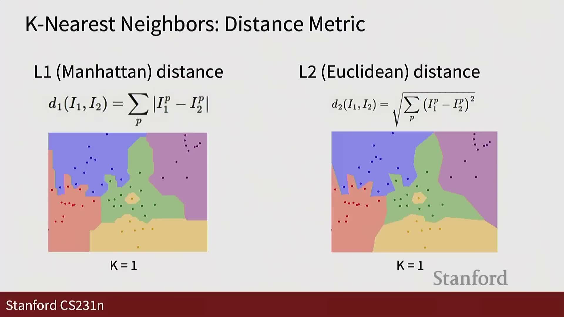
Visualization insight: L1 and L2 yield different partition boundaries in 2D feature space.
-
L1 tends to produce axis-aligned boundaries and can change substantially with feature rotation.
-
L2 yields smoother, radial boundaries and is invariant under orthonormal rotations.
Advice: experiment with both metrics and with feature representations; interactive visual tools help explore these effects and build intuition about metric-feature interactions.
Hyperparameters in k-NN and general model selection
Hyperparameters are design choices not learned during standard training (e.g., k, distance function).
- Their optimal values depend on dataset characteristics.
- Naive strategies are problematic:
- Tuning on training data leads to overfitting (e.g., k=1 memorizes training).
- Tuning on the test set leaks information and invalidates evaluation.
- Tuning on training data leads to overfitting (e.g., k=1 memorizes training).
Solution: use a separate validation set or cross-validation to estimate generalization performance for hyperparameter selection.
Validation, testing, and cross-validation for hyperparameter tuning
A robust hyperparameter selection workflow:
-
Reserve a validation set distinct from training and test sets. Tune hyperparameters on validation performance.
-
Evaluate final performance once on a held-out test set to report generalization.
- For smaller problems, use k-fold cross-validation on the training set to reduce variance: partition training data into folds, cycle which fold serves as validation, and aggregate results.
Practical note: cross-validation is computationally expensive for large-scale deep learning, where single validation splits and practitioner intuition are often used instead.
Introduction to the CIFAR-10 dataset and k-NN qualitative results
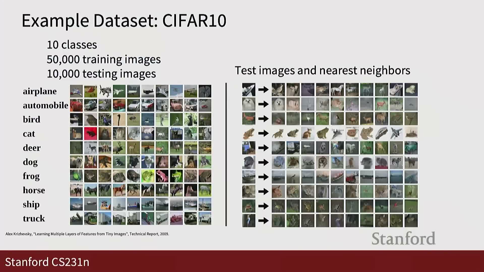
The CIFAR-10 dataset is introduced as a standard 10-class benchmark used in assignments.
- Example experiments show nearest-neighbor retrievals where top-k neighbors are visualized for query test images.
- Retrieving neighbors offers intuition about what the classifier deems similar and reveals systematic failure modes when similarity is computed by pixel distances.
Positioning: CIFAR-10 provides a concrete demonstration of k-NN behavior on a small but realistic vision dataset.
Empirical k selection on CIFAR-10 and baseline accuracy
Empirical result on CIFAR-10 (five-fold validation):
- Best validation accuracy found near k ≈ 7, with accuracy around 28%.
- This substantially outperforms random guessing (10%) but leaves considerable room for improvement.
Interpretation: the validation curve over k quantifies the bias–variance trade-off in neighbor voting and motivates stronger features and learned models to reach modern performance levels.
Failure modes of pixel-wise distances and translation sensitivity
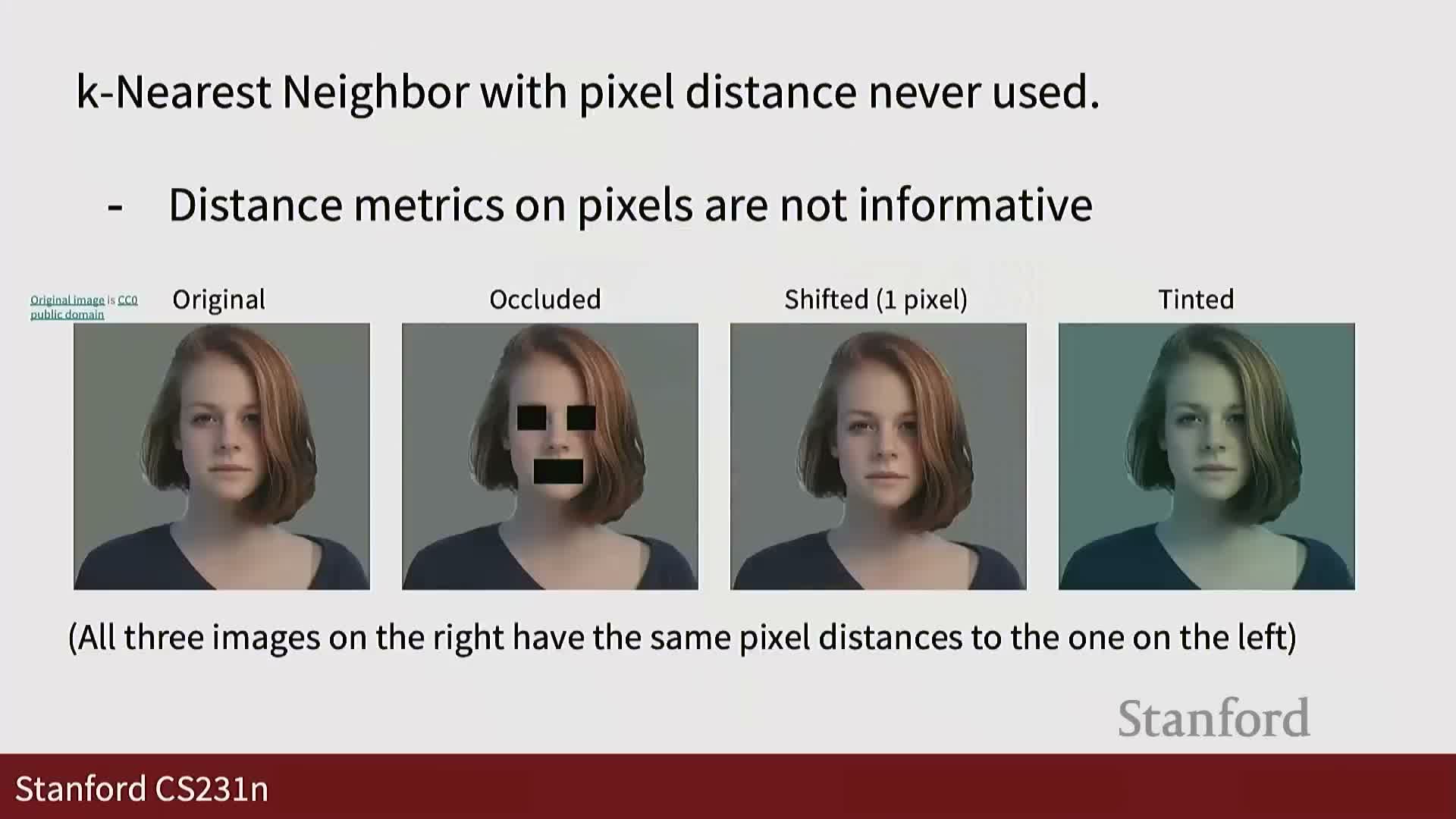
Concrete failure modes of pixel-based similarity:
- Pixel-wise distances can retrieve perceptually dissimilar images and are highly sensitive to small translations, color changes, or occlusions.
- Small geometric shifts (even one-pixel translations) can produce the same distance as radical semantic changes.
Conclusion: pixel-level similarity is a poor proxy for semantic similarity and motivates representation learning and feature extraction that are invariant to irrelevant transformations.
Transition to linear classifiers as parametric models
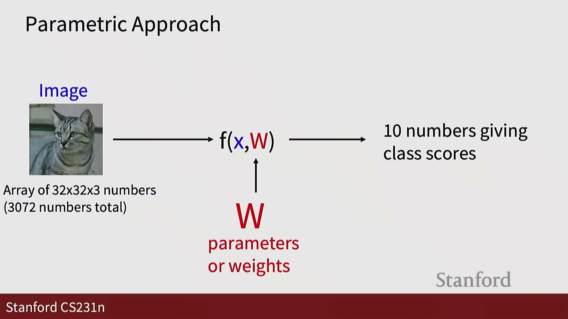
Transition to parametric linear classifiers:
- Linear classifiers learn a parameter matrix W (and often a bias b) to map input vectors directly to per-class scores.
- These learned linear maps are essential building blocks for deep learning architectures and can be converted into probabilistic outputs for downstream loss functions.
This sets up the following exposition on parameterization, geometric interpretations, and optimization to fit W to training data.
Parameterization of linear classifiers: weight matrix and bias
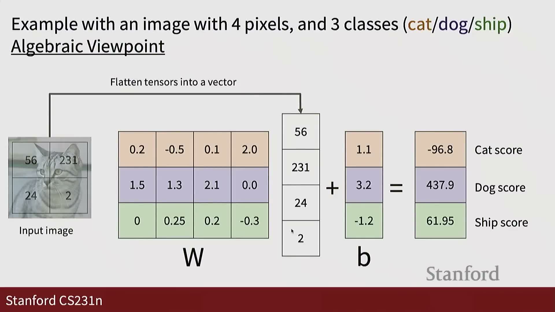
Algebraic formulation of a linear classifier:
- Flatten a high-dimensional input image into a vector x (e.g., 32 × 32 × 3 → D features).
- Compute class scores with a weight matrix W and optional bias b, producing a C-dimensional score vector for C classes.
- Dimensions: W is C × D; each row of W is a linear template or scoring function for one class.
Role of bias: b provides score offsets independent of input magnitude, increasing decision-boundary flexibility.
Linear models as foundational components of neural networks
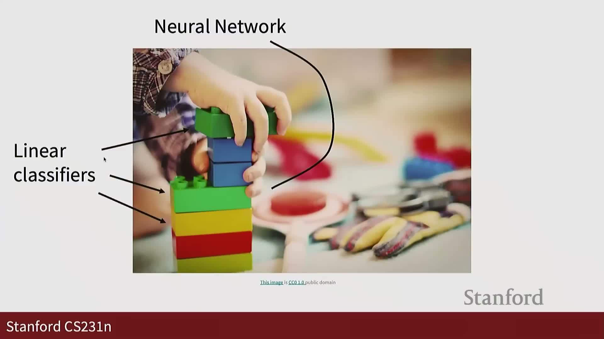
Linear functions are the ubiquitous basic unit in neural network architectures.
- Stacked linear layers without nonlinearity remain equivalent to a single linear transform.
- When combined with nonlinear activation functions, linear layers become powerful building blocks for deep models capable of complex representations.
Understanding linear classifiers is therefore essential background for later material on multilayer networks and convolutional architectures.
Simplified 2×2 image example to illustrate linear scoring
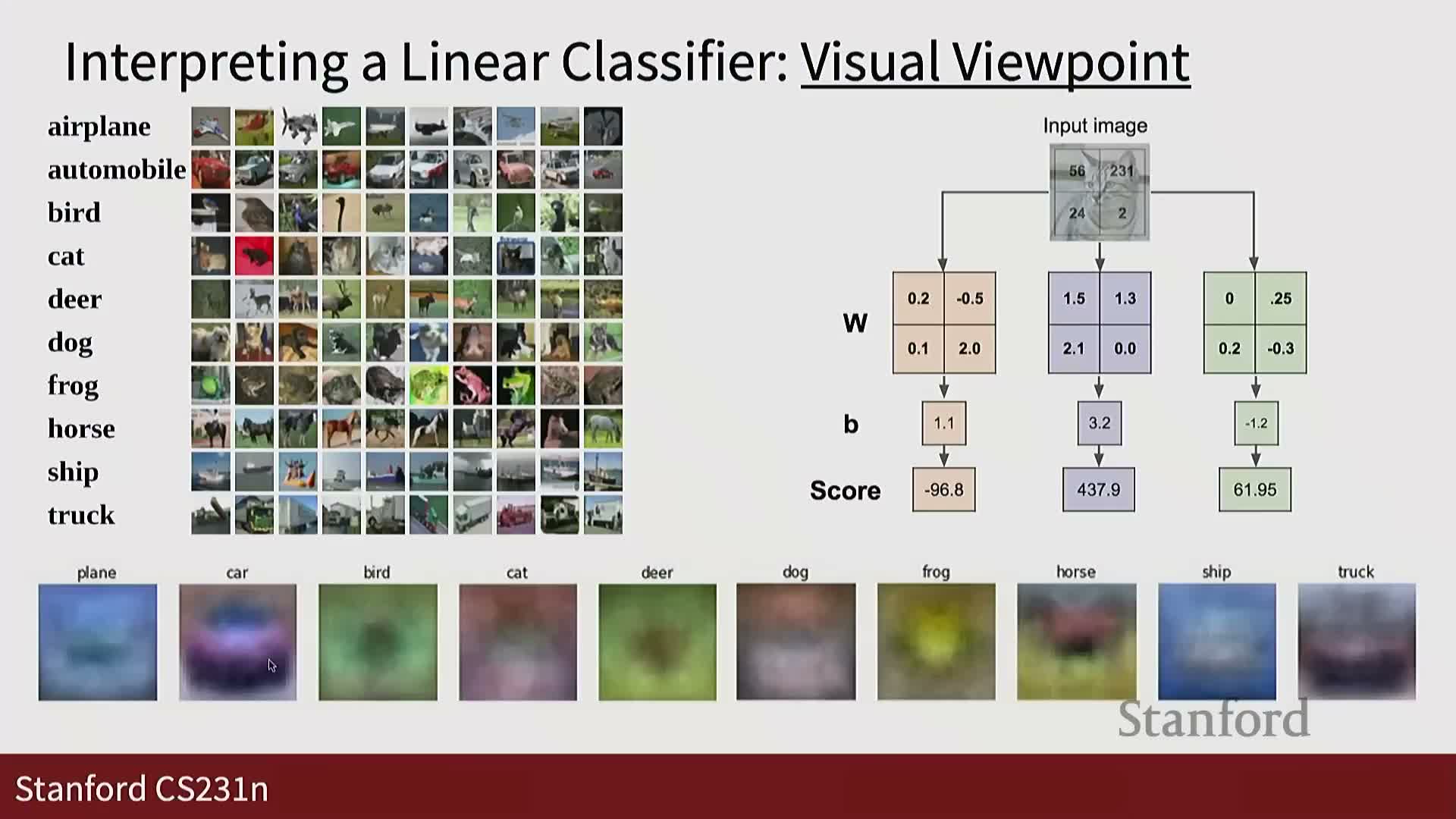
A concrete toy example: a 2×2 image flattened into a 4-dimensional input vector mapped to a 3-class output.
- The linear scoring function computes class scores by matrix multiplication and bias addition.
- Each row of W, reshaped, can be interpreted as a class-specific template over the 2×2 pixels.
This simplified setting aids intuition about parameter roles, score interpretation, and geometric behavior of linear classifiers.
Visual templates and geometric decision boundaries for linear classifiers
Two complementary perspectives on linear classifiers:
-
Template view: each learned row of W can be reshaped into an image-like filter that looks like a class prototype or template.
-
Geometric view: classifiers partition feature space with hyperplanes; the bias shifts hyperplanes away from the origin.
Both perspectives illuminate different aspects of model behavior—templates help interpret pixel-level patterns, while geometry clarifies how classes are separated in high-dimensional space.
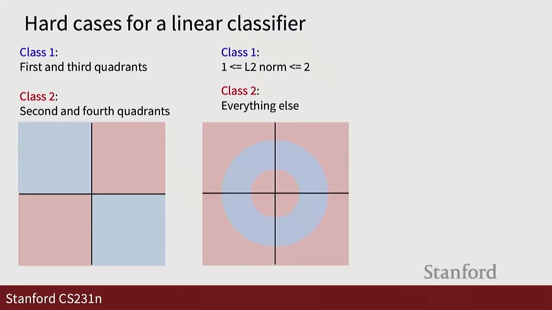
Limitations of linear separability
Limitations of linear classifiers:
- They cannot solve XOR-like configurations or multi-modal class distributions requiring non-linear separation.
- Examples include classes occupying multiple disconnected regions or one class enclosing another—no single affine separator can partition such spaces correctly.
Motivation: these failures demonstrate the need for nonlinear transformations or multi-layer architectures to model complex decision boundaries.
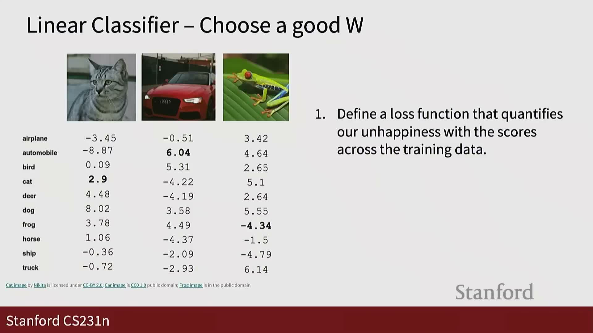
Role of a loss function and optimization objective
Introduce the concept of a loss (objective) function:
- A loss quantifies classifier error on labeled training examples.
-
Optimization adjusts weights W to minimize this loss, providing the training signal needed to learn from data.
This sets the stage for introducing the softmax classifier and cross-entropy loss as principled choices for multiclass problems; optimization algorithms to minimize these losses are discussed in later lectures.
Softmax transformation: converting logits to class probabilities

The softmax function maps raw class scores (logits) to a probability distribution over classes.
- Mechanism: exponentiate logits (ensures positive outputs) and normalize by their sum (ensures unit total probability).
- Result: bounded, interpretable probabilities that indicate model confidence for each class.
Terminology: pre-softmax values are often called logits; softmax outputs are suitable inputs to probabilistic loss functions.
Negative log-likelihood (softmax loss) and relation to logistic regression
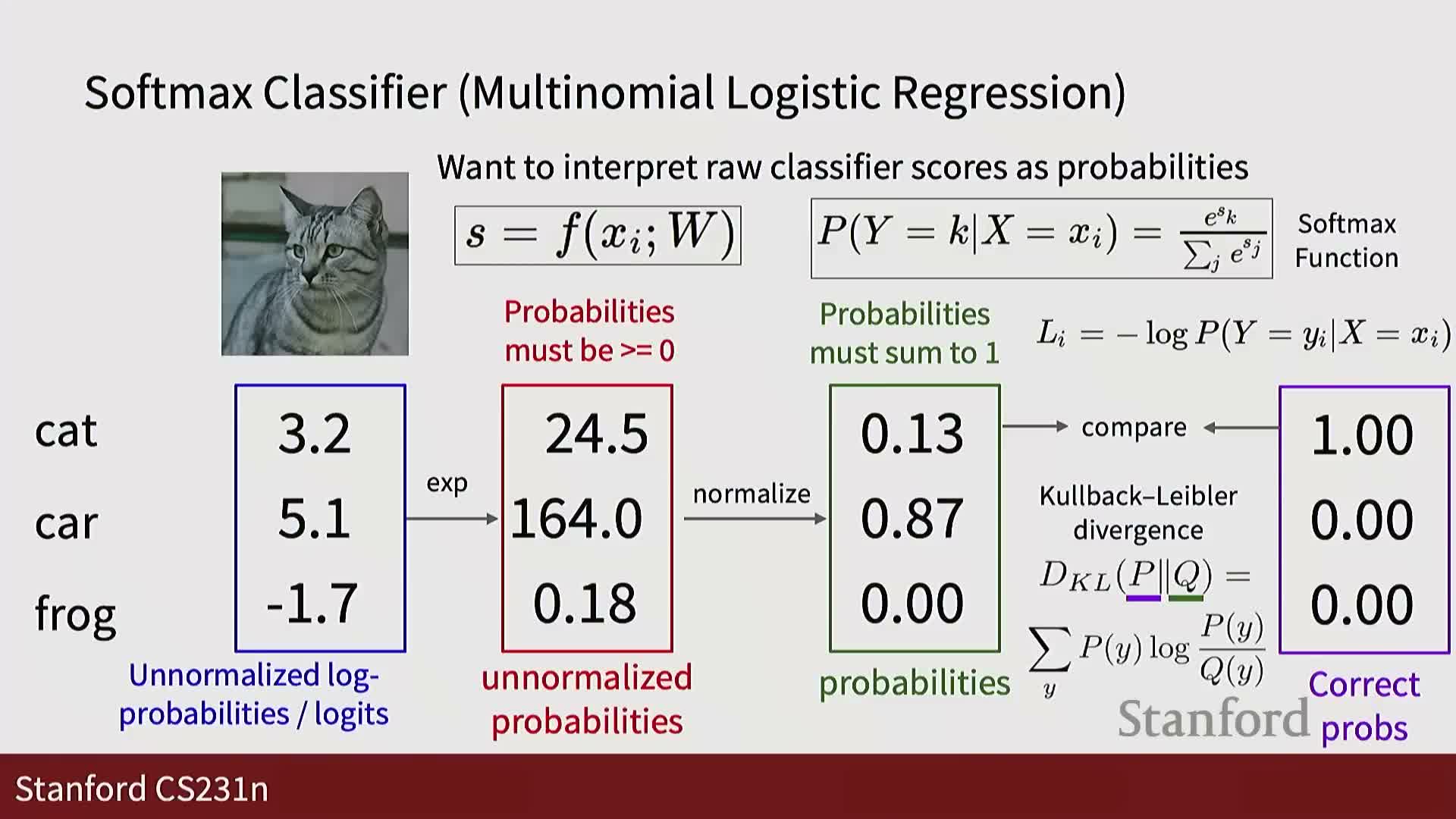
The softmax loss (negative log-likelihood) is defined as the negative log probability assigned to the correct class.
- Minimizing this loss is equivalent to multinomial logistic regression and to maximum likelihood estimation under a categorical model.
- Intuition: minimizing negative log-likelihood encourages the model to allocate high probability mass to the ground-truth class for each training example.
This formulation provides a principled objective for multiclass classification in statistical learning frameworks.
Information-theoretic interpretations: KL divergence and cross-entropy

Equivalent interpretations of the softmax loss from information theory:
- Minimizing the softmax loss is equivalent to minimizing the KL divergence between the empirical one-hot label distribution and the model distribution.
- Equivalently, it minimizes cross-entropy between target and predicted distributions; with one-hot targets this reduces to the negative log probability of the correct class.
These equivalences ground the softmax objective in principled divergence measures and justify calling it cross-entropy loss in practice.
Enjoy Reading This Article?
Here are some more articles you might like to read next: