Stanford CS231N | Spring 2025 | Lecture 3- Regularization and Optimization
- Lecture overview and image classification task
- Main visual recognition challenges for image classification
- K-nearest neighbors and dataset splits for hyperparameter selection
- Linear classifiers as matrix multiplications and multiple viewpoints
- Loss functions and softmax cross-entropy for classification
- Regularization objective and the bias–variance trade-off
- L2 versus L1 regularization and their effects on weights
- How regularization guides optimization and model selection
- Softmax usefulness and interaction between regularization and model simplicity
- Overview of optimization goal and baseline parameter search
- Gradient and gradient descent fundamentals
- Numerical gradient checking as a debugging tool
- Stochastic gradient descent and mini-batch training
- Common optimization pathologies: poor conditioning, oscillation, and saddle points
- Momentum accelerates optimization by accumulating velocity
- RMSProp implements per-parameter adaptive learning rates via squared-gradient averaging
- Adam optimizer combines momentum and RMSProp with bias correction
- Practical defaults, implementation caveats, and optimizer selection
- Interaction of regularization and optimizer; learning rate schedules and scaling
- Second-order optimization and practical limitations in deep learning
- Concluding practical recommendations and preview of neural networks
Lecture overview and image classification task
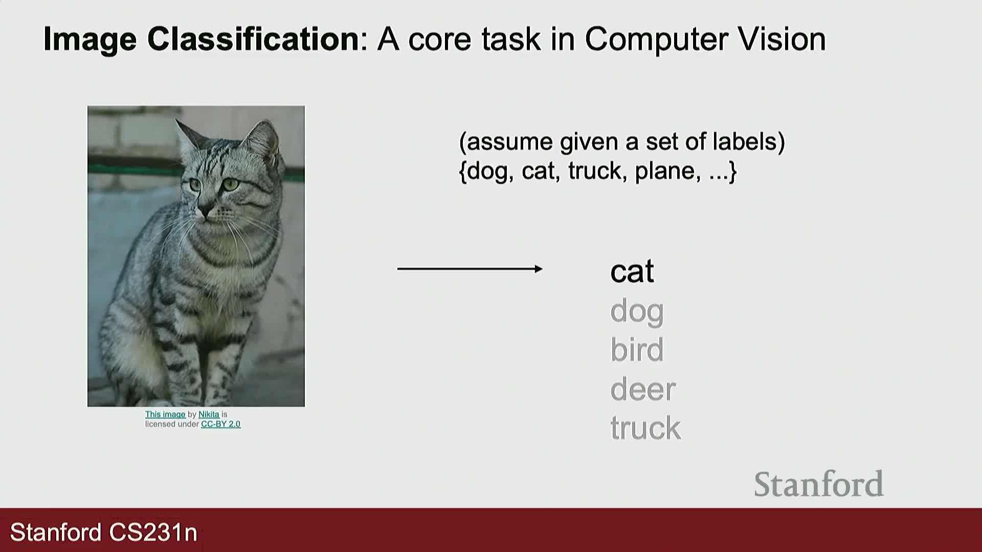
The lecture introduces regularization and optimization as core concepts in machine learning with particular emphasis on computer vision.
Image classification is defined as a mapping from raw image input to a discrete label drawn from a predefined set, implemented by a parametric model (a function that transforms an image tensor into class outputs).
Typical image inputs are represented as multi-dimensional arrays of pixel intensities (e.g., width × height × channels).
Learning algorithms must bridge the semantic gap between pixel grids and human-recognizable categories—this task formulation is the foundation for later discussions on modeling, loss design, and training procedures.
Main visual recognition challenges for image classification
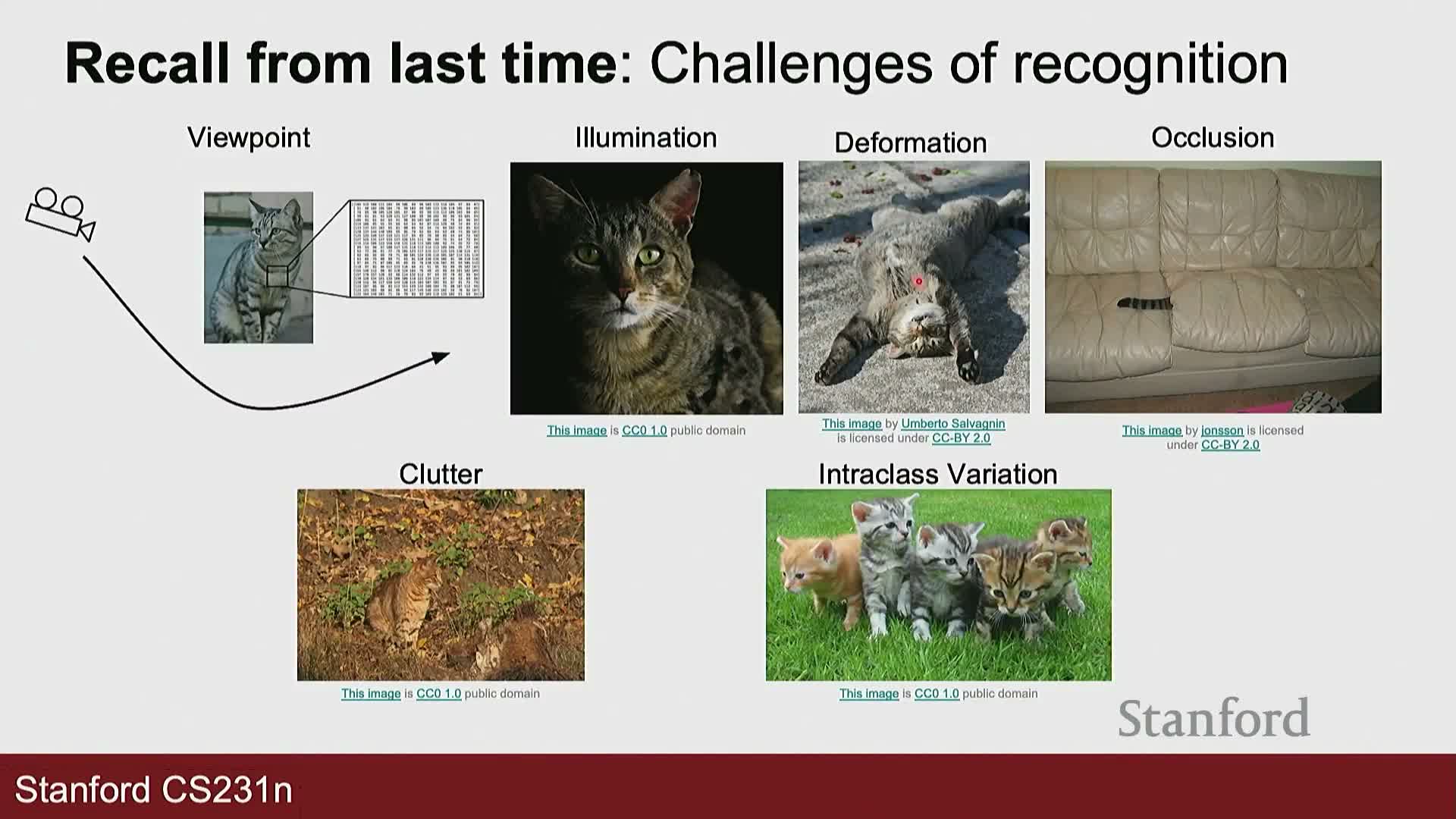
Image classification faces multiple intrinsic challenges:
-
Illumination variation and shadows change pixel intensity distributions, confusing pixel-level similarity.
-
Deformability: objects (e.g., animals) change shape and pose, altering appearance across instances.
-
Occlusion and background clutter can obscure salient features, breaking simple heuristics.
-
Intra-class variability: members of the same class can look very different, requiring broad generalization.
Simple rule-based methods are therefore insufficient; robust classifiers require data-driven learning that captures complex invariances and statistical regularities from training data.
K-nearest neighbors and dataset splits for hyperparameter selection
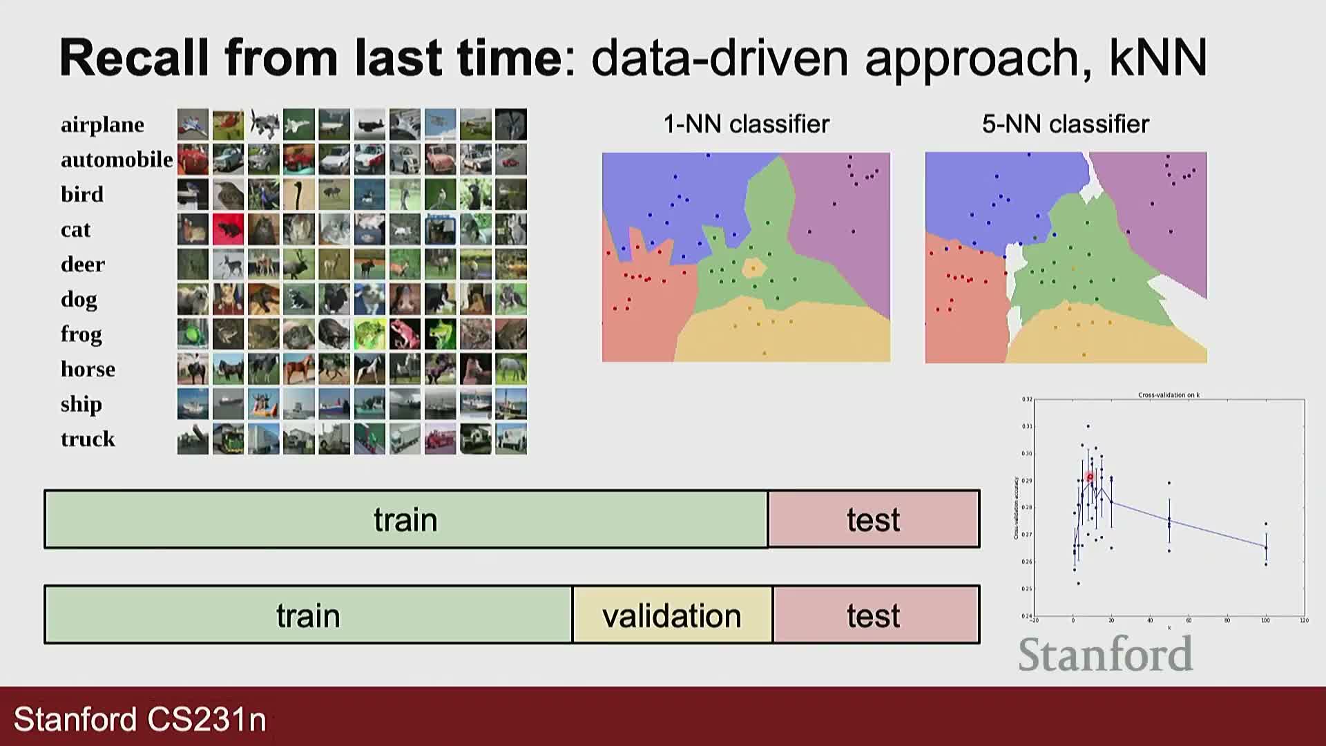
k-nearest neighbors (kNN) is presented as a simple data-driven baseline:
- Class assignment is determined by labels of the closest training examples under a chosen distance metric.
- Standard dataset partitions: train, validation, and test splits—use the validation set to select hyperparameters (e.g., k) and the test set to estimate final generalization.
- Common distance metrics: L1 (Manhattan) and L2 (Euclidean).
- Geometric effects of metrics:
-
L2 equidistance loci form circles (or hyperspheres) in input space.
-
L1 equidistance loci form diamond-shaped (octahedral) regions.
-
L2 equidistance loci form circles (or hyperspheres) in input space.
- Proper dataset partitioning and metric selection are practical prerequisites for reproducible performance estimation.
Linear classifiers as matrix multiplications and multiple viewpoints
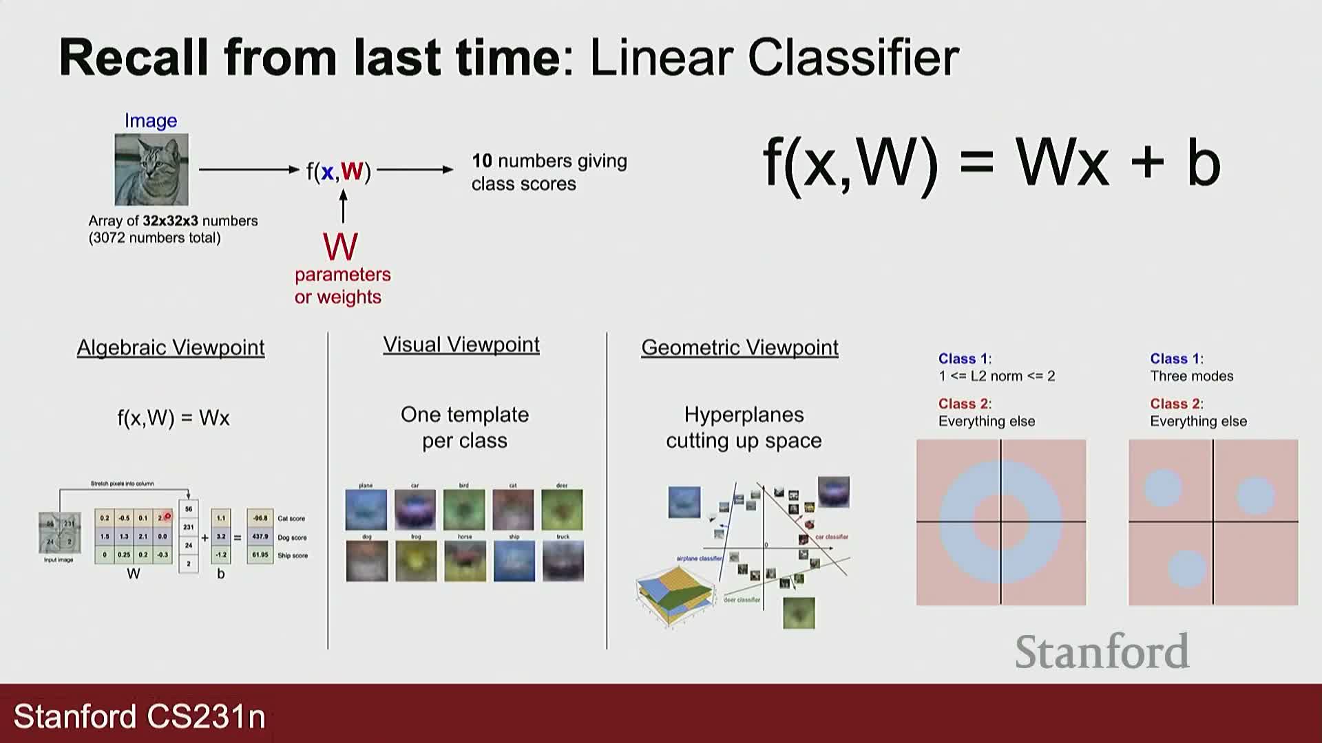
Linear classifiers compute class scores by flattening an image into a vector x and multiplying by a weight matrix W (plus optional bias), producing a score vector whose largest element indicates the predicted class.
Three equivalent viewpoints clarify intuition:
-
Algebraic view: each row of W is an independent linear classifier for one class—scores are dot products between row vectors and x.
-
Template view: reshape each row of W into an image-shaped template that scores similarity with the input image.
-
Geometric view: rows of W define hyperplanes in input space; their signs and intersections form decision boundaries.
These perspectives explain the simple implementation (a matrix multiply) and the limitations (many class distributions are not linearly separable) of linear models in high-dimensional input spaces.
Loss functions and softmax cross-entropy for classification
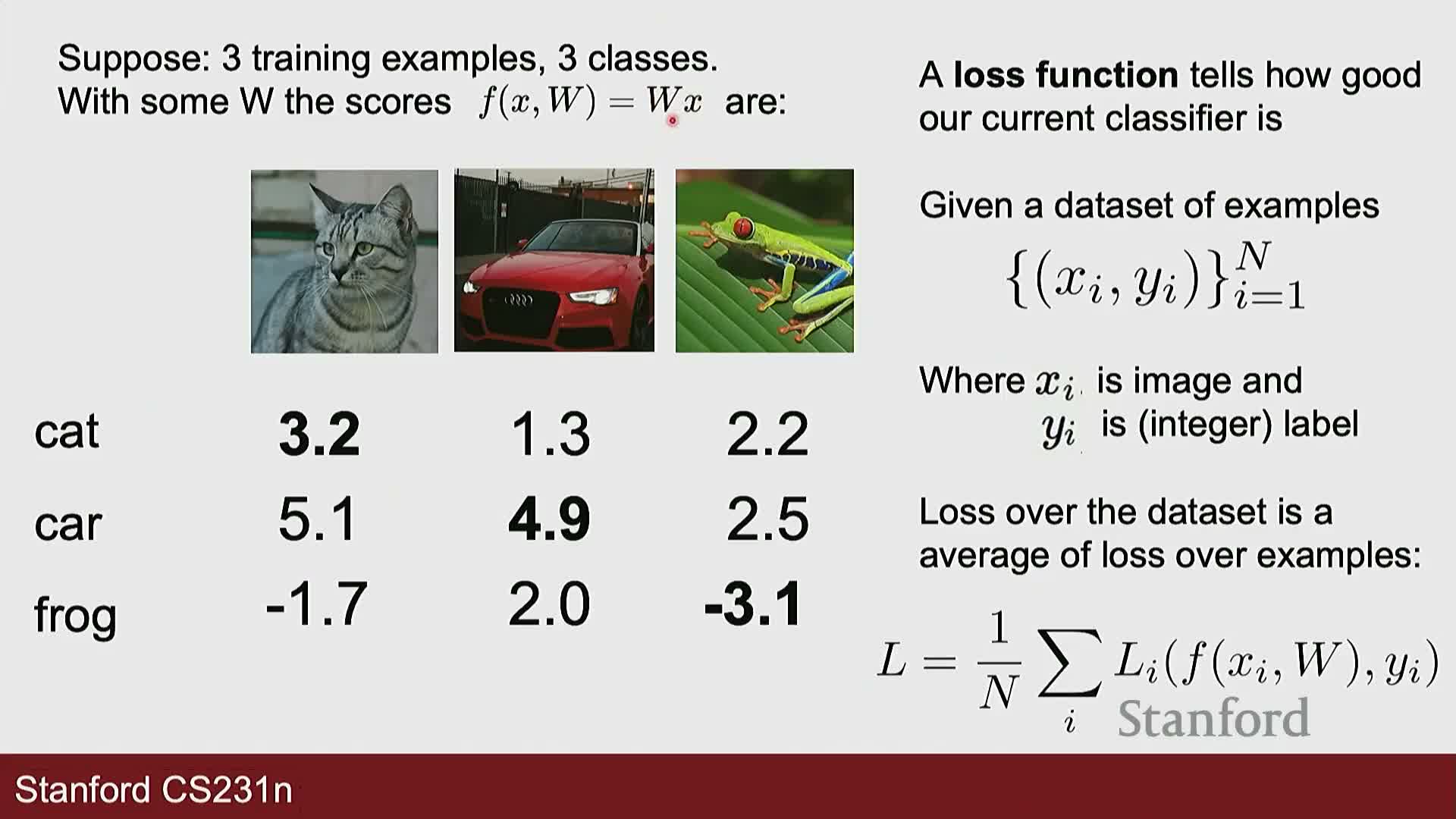
A loss function quantifies how poorly a model’s predictions match ground-truth labels and provides the scalar objective to minimize during learning.
For multiclass classification, the softmax followed by cross-entropy (log loss) converts raw class scores into a probability distribution by exponentiating scores and normalizing, then penalizes low predicted probability on the true class via negative log-likelihood.
The dataset-level loss is the average of per-example losses plus optional regularization; the data loss measures fit to training labels while the regularization term encodes inductive preferences over parameters.
Choosing an appropriate loss yields gradients that guide parameter updates via optimization algorithms.
Regularization objective and the bias–variance trade-off
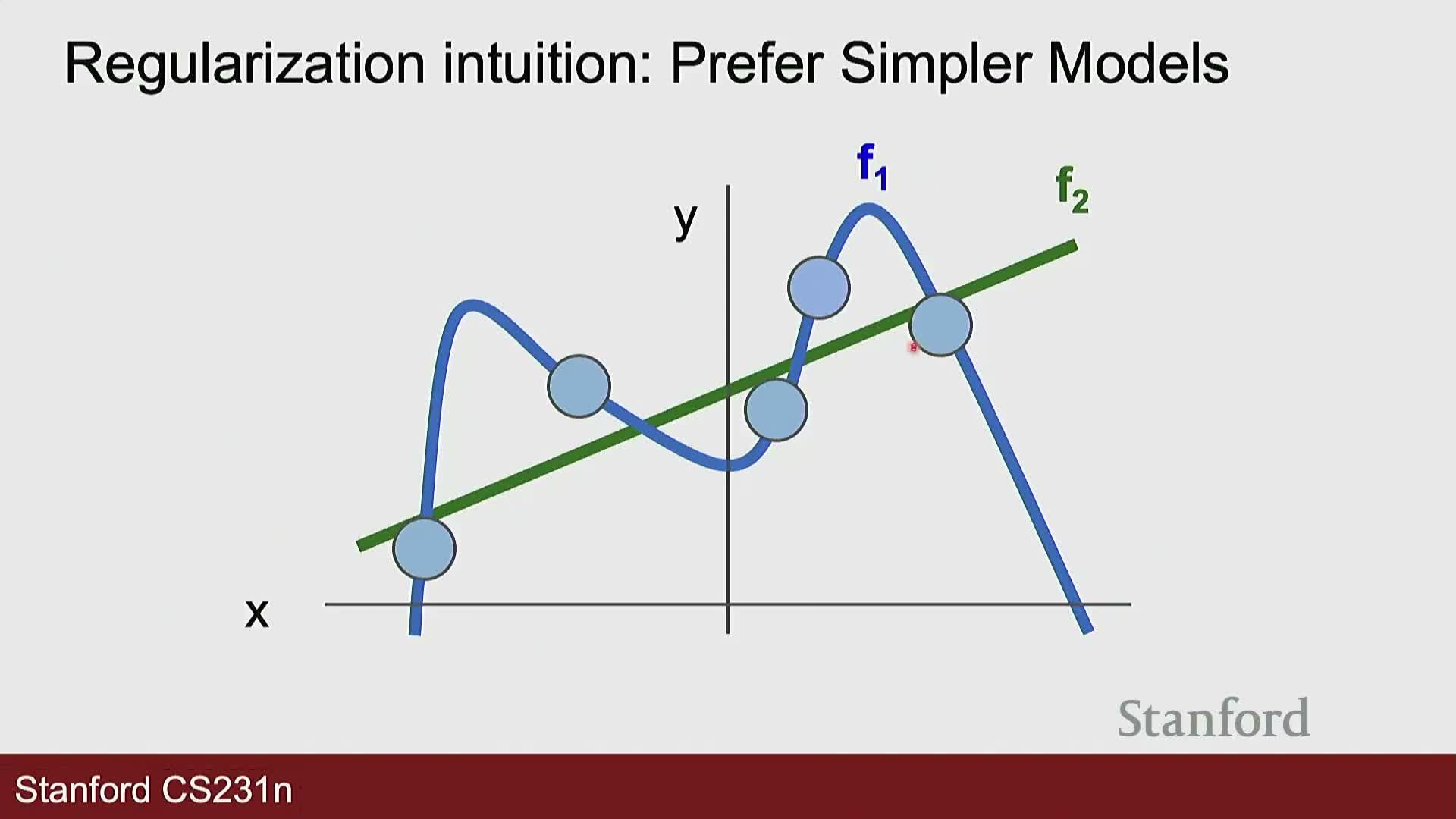
Regularization augments the data loss with a penalty term on model parameters to discourage overfitting, trading potentially higher training error for improved test-time generalization.
- The strength of regularization is controlled by a hyperparameter λ that balances data loss and regularization: λ = 0 recovers unregularized training, while very large λ enforces strong prior bias on parameter magnitudes.
- Intuition: models that fit noise or high-frequency patterns (high variance) are penalized in favor of simpler or more stable solutions expected to generalize better—an application of Occam’s razor in practice.
Select λ by validation to achieve the desired bias–variance tradeoff.
L2 versus L1 regularization and their effects on weights

L2 regularization and L1 regularization impose different structural preferences on parameters:
-
L2 (sum of squared parameters)
- Encourages small but distributed (dense) weights because squaring disproportionately penalizes large values and less so already-small parameters.
- Tends to produce many small nonzero coefficients—good for smooth, distributed representations.
- Encourages small but distributed (dense) weights because squaring disproportionately penalizes large values and less so already-small parameters.
-
L1 (sum of absolute values)
- Encourages sparsity because the linear penalty makes zero-valued parameters a favored solution when they do not harm data loss.
- Useful for feature selection, interpretability, or sparse connectivity.
- Encourages sparsity because the linear penalty makes zero-valued parameters a favored solution when they do not harm data loss.
Practically, choose L2 when you want spread-out representations and L1 when you expect or desire sparse solutions.
How regularization guides optimization and model selection

Regularization directly modifies the optimization objective, so models are obtained by minimizing the joint objective (data loss + regularizer).
- The optimizer naturally trades off fitting the data versus reducing the regularizer: if changing a weight negligibly affects data loss but reduces the regularization penalty, the joint objective favors that change.
- Conversely, weights that substantially improve data loss will be kept despite some regularization cost.
- Regularization can also improve optimization properties (for example, L2 adds quadratic curvature that helps convex optimization).
Always tune regularization strength on a validation set to select appropriate λ values.
Softmax usefulness and interaction between regularization and model simplicity

Softmax converts arbitrary real-valued class scores into a normalized probability distribution, enabling probabilistic interpretation and computation of cross-entropy loss for training classifiers.
Regularizers target different notions of simplicity:
-
L1 / L2 impose structural priors on parameter magnitudes (sparsity vs spread) but do not universally make models “simpler” in every sense.
- Other regularizers—dropout, architectural constraints (e.g., bottlenecks, weight sharing)—alter model capacity or effective complexity in different ways.
Choose regularization methods that reflect domain priors about desirable parameter structure and generalization behavior.
Overview of optimization goal and baseline parameter search

Optimization seeks the parameter set W that minimizes the chosen loss landscape—a high-dimensional surface whose coordinates are parameter values and elevation is loss.
- A brute-force baseline is random search over parameter samples: simple, but extremely inefficient and poor in high-dimensional settings.
- Effective optimization requires gradient-based or curvature-aware methods that leverage local derivative information to navigate toward minima far more efficiently than random sampling.
Gradient and gradient descent fundamentals
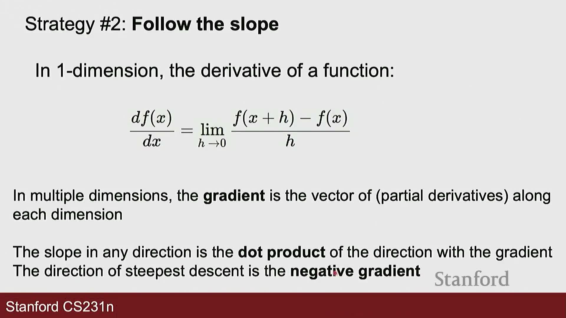
The gradient generalizes the derivative to multi-dimensional parameter spaces and points in the direction of steepest increase; the negative gradient is therefore the direction of steepest decrease and is used for minimization.
-
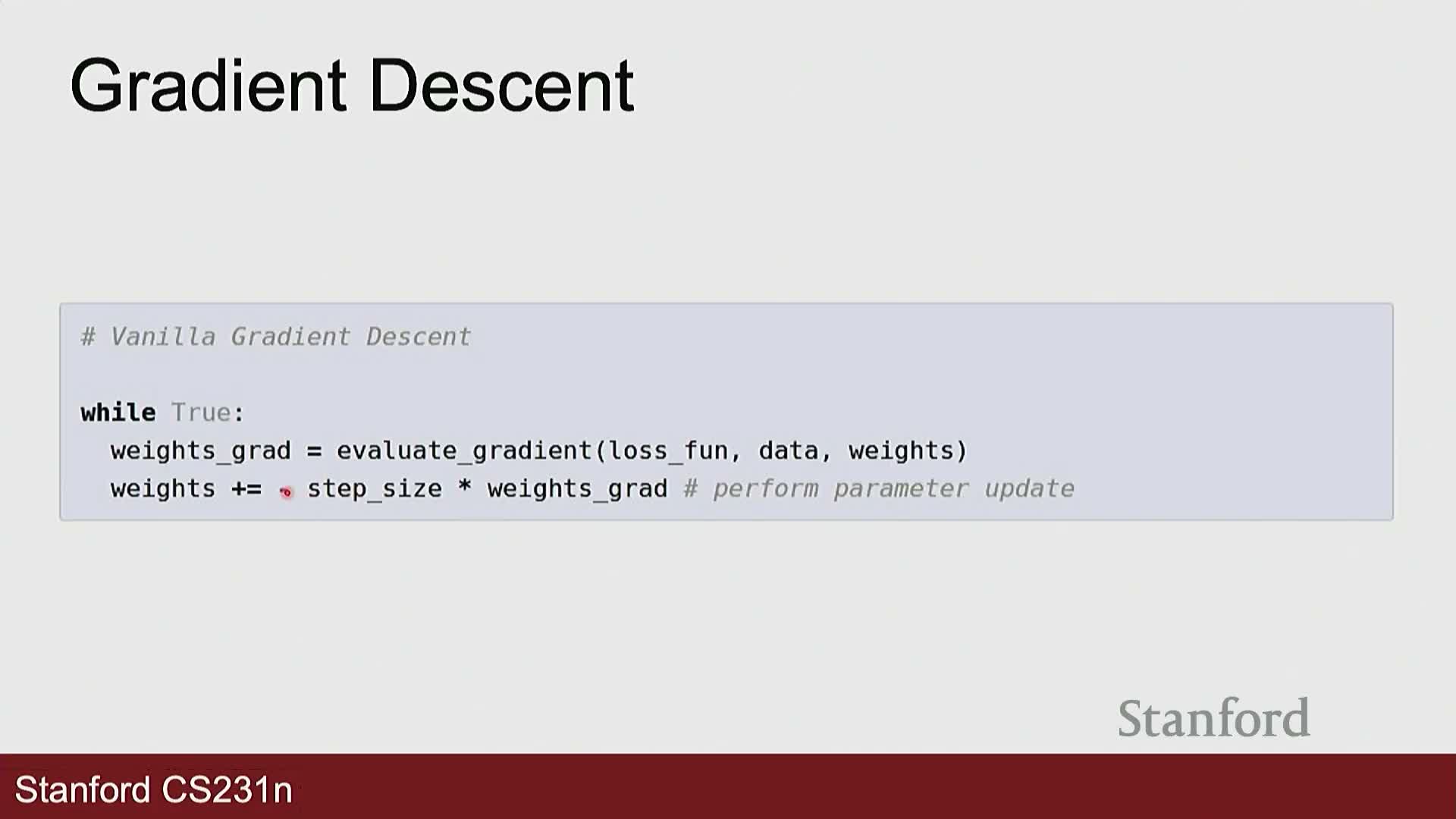
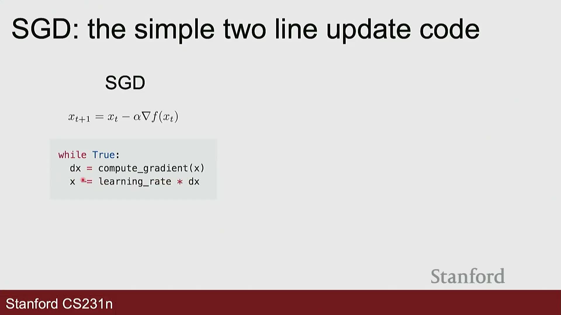
Gradient descent updates parameters by stepping in the negative gradient direction scaled by a learning rate α, iteratively reducing loss.
- Algorithmic choices include step size selection, stopping criteria, and initialization.
- Accurate gradients can be computed analytically via the chain rule (symbolic differentiation), which is exact and efficient compared to finite-difference numerical gradients that are slow and error-prone.
Numerical gradient checking as a debugging tool
Finite-difference numerical gradients approximate partial derivatives by perturbing each parameter by a small h and computing loss differences—useful as a correctness check for analytic gradients.
- Numerical gradients are computationally expensive (cost ∝ number of parameters) and less precise, but they serve as an effective gradient-checking tool during implementation.
- Small discrepancies between analytic and numerical gradients typically indicate coding errors; rigorous gradient checks are standard practice in assignments and component development.
Stochastic gradient descent and mini-batch training
Stochastic gradient descent (SGD) approximates full-batch gradients by computing gradients on small randomly sampled mini-batches, drastically reducing per-update computation and enabling scalable training.
- One epoch is a single pass through the entire dataset using shuffled mini-batches; repeated epochs let the optimizer see the whole dataset multiple times.
- Mini-batch SGD introduces gradient noise that can help escape shallow local minima and saddle points, but also adds variance in update directions that must be managed via learning rate scheduling, momentum, or adaptive methods.
Common optimization pathologies: poor conditioning, oscillation, and saddle points
Gradient-based optimizers encounter several pathologies in nontrivial loss landscapes:
-
Poorly conditioned valleys: large curvature disparity causes oscillation across steep directions and tiny progress along flat directions.
-
Too-large learning rates: can produce overshooting and divergence.
-
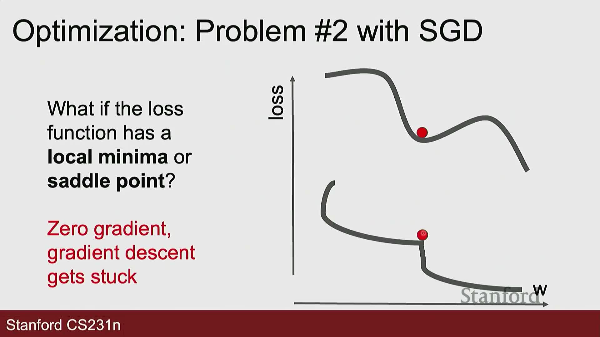
Saddle points and flat regions: near-zero gradients stall progress; saddle points are especially common in high-dimensional parameter spaces.
Algorithmic mechanisms—momentum, injected noise, or curvature-aware updates—help maintain progress toward useful minima.
Momentum accelerates optimization by accumulating velocity

Momentum augments gradient descent with a velocity vector that accumulates an exponentially weighted average of past gradients, producing updates that blend current gradient information with historical directionality.
- The momentum coefficient β controls how much past velocity is retained; larger β yields smoother trajectories that can traverse small local minima and damp oscillations in high-curvature directions.
- Intuition: momentum acts like inertia for a ball rolling down the loss landscape, enabling faster convergence along consistent directions while averaging out stochastic gradient noise.
RMSProp implements per-parameter adaptive learning rates via squared-gradient averaging
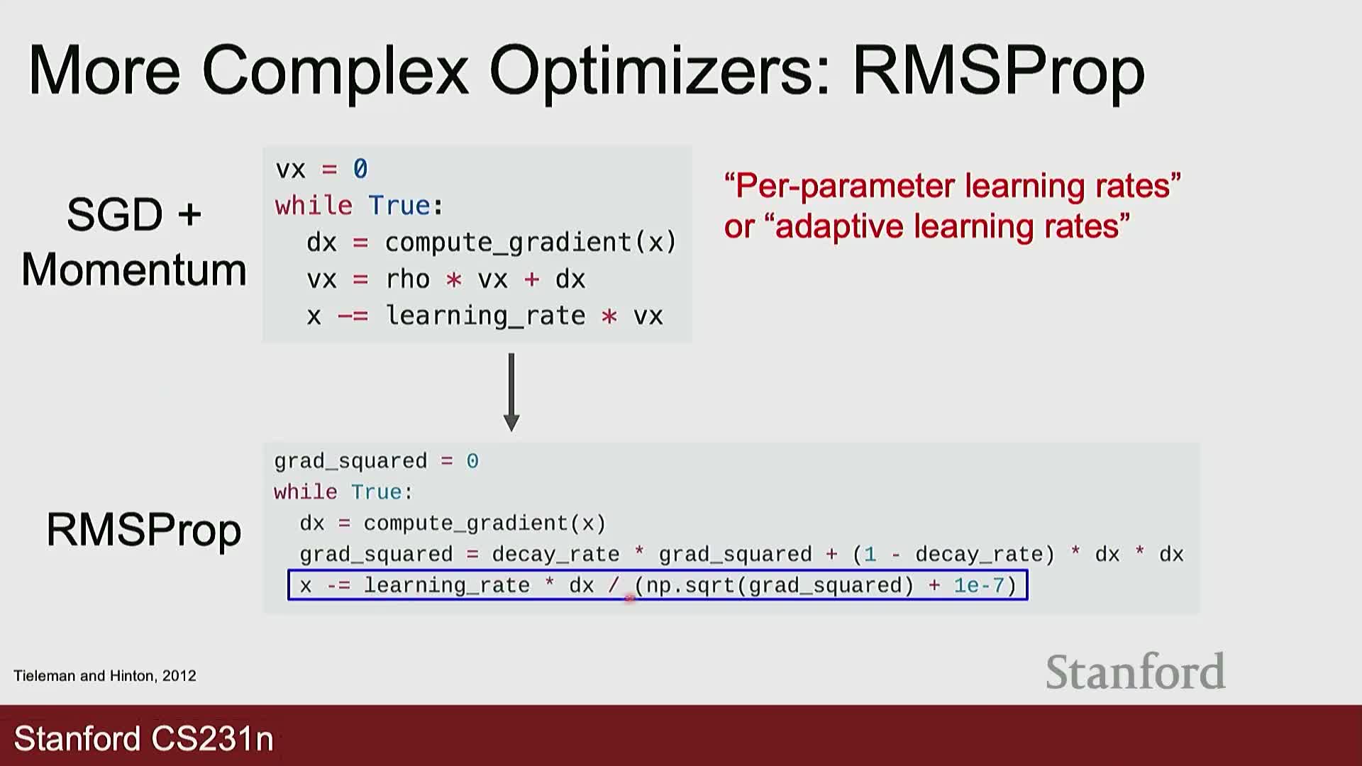
RMSProp maintains an exponential moving average of squared gradients for each parameter and divides the gradient by the square root of this average, producing elementwise adaptive step sizes.
- Parameters with consistently large gradients receive proportionally smaller updates; parameters with small gradients get relatively larger effective steps.
- This addresses poor conditioning and reduces oscillation along steep axes, improving empirical convergence in many deep networks.
Adam optimizer combines momentum and RMSProp with bias correction
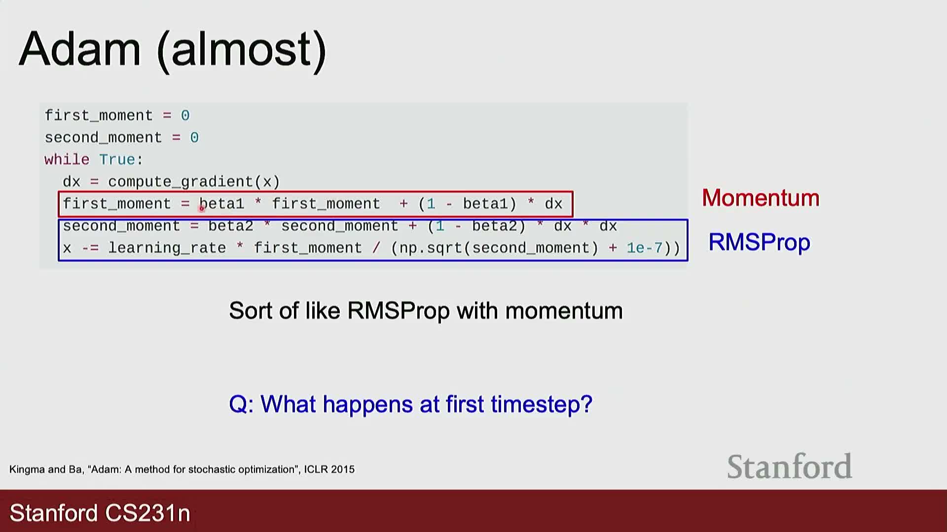
Adam integrates first-moment (momentum-like) and second-moment (RMSProp-like) exponential moving averages to provide adaptive, momentum-augmented, per-parameter learning rates.
- Adam requires bias-correction terms in early iterations because the exponential moving averages initialized at zero introduce a time-step dependent bias that would otherwise yield excessively large initial updates.
- Typical hyperparameters that work well in practice: β1 ≈ 0.9, β2 ≈ 0.999, and a small ε for numerical stability.
-
AdamW is a variant that decouples weight decay from moment estimates, implementing L2-style regularization as direct weight decay and often improving empirical performance.
Practical defaults, implementation caveats, and optimizer selection
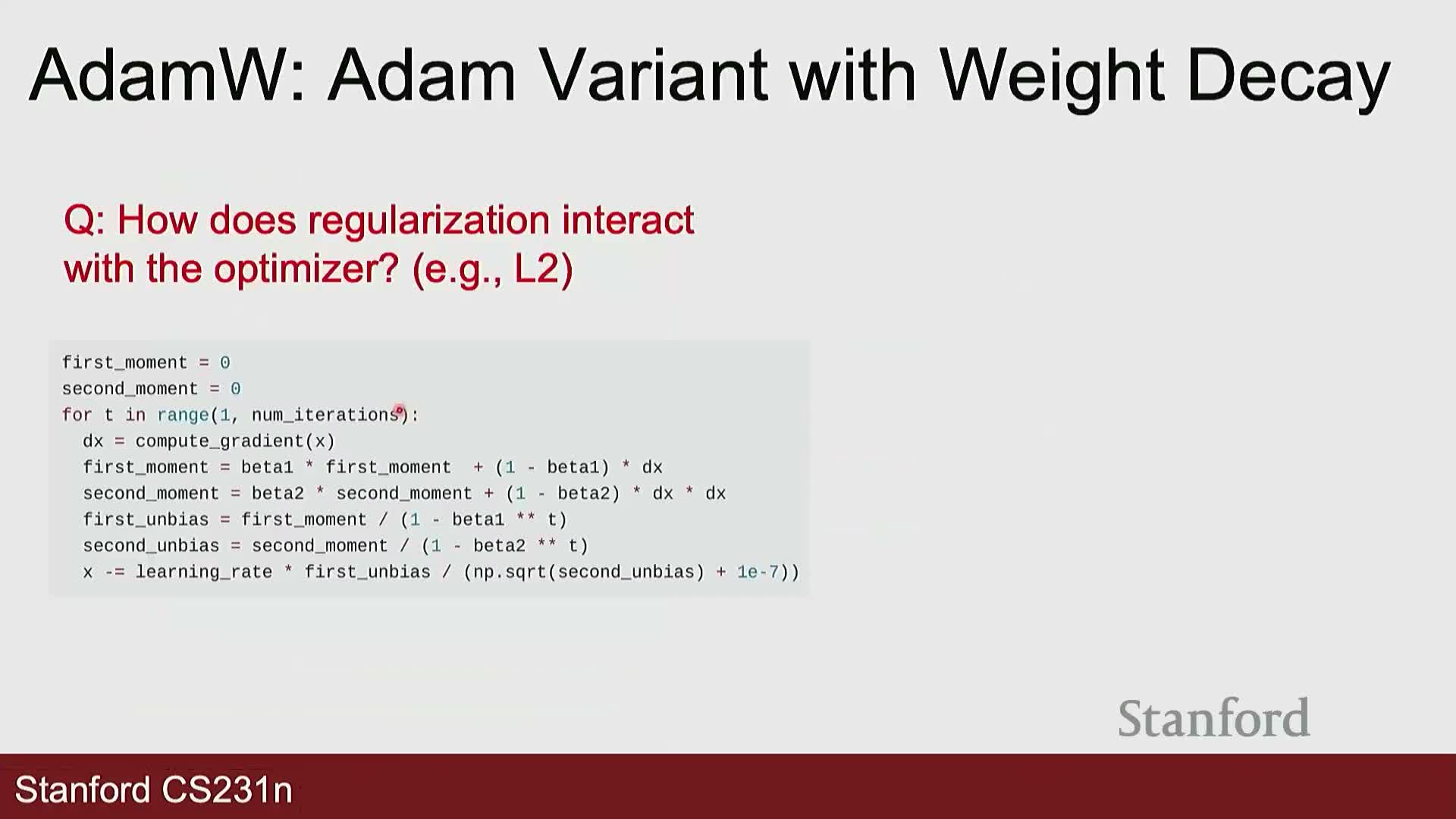
Use Adam or AdamW as a strong default optimizer for new problems because they adapt to varying gradient scales and reduce the need for extensive hand-tuning.
-
SGD with momentum can outperform adaptive methods in some large-scale vision tasks when carefully tuned; optimizer choice should be validated empirically.
- Implementation details matter: bias-correction, epsilon stabilization, and whether L2 regularization is applied inside moment computations versus as decoupled weight decay (AdamW) affect training dynamics.
- Perform empirical evaluation across random seeds and hyperparameter sweeps to select optimizers and schedules that generalize well for your model and dataset.
Interaction of regularization and optimizer; learning rate schedules and scaling
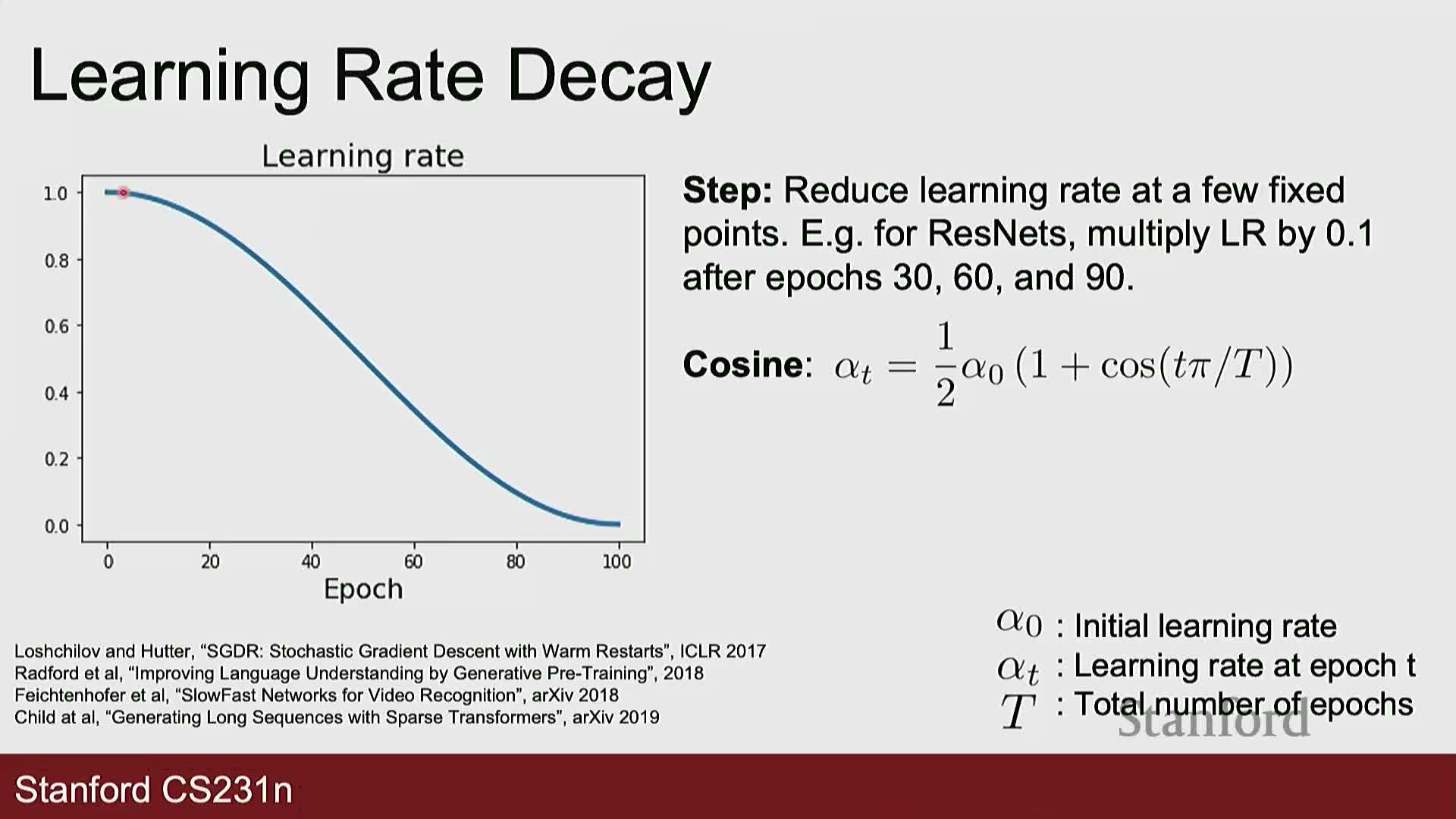
Regularization can be incorporated either directly into gradient computations or applied as decoupled weight decay; this design choice affects optimizer internal statistics and empirical performance—AdamW implements the decoupled approach with practical benefits.
Learning rate selection is critical:
- Too large → divergence; too small → slow convergence.
- Common dynamic schedules: step decay, cosine decay, linear warm-up, inverse-sqrt, etc., trade initial speed for later fine convergence.
- Practical scaling rule: linear scaling of learning rate with batch size—if batch size increases by factor n, increasing the learning rate by n often preserves or improves training behavior when other settings are adjusted accordingly.
Second-order optimization and practical limitations in deep learning
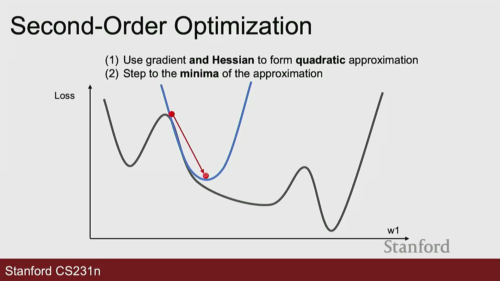
Second-order methods use curvature information (the Hessian or approximations) to form local quadratic models and compute updates that account for varying curvature across directions, enabling potentially larger and more accurate steps.
- Exact Hessian computation and inversion is computationally and memory prohibitive for modern neural networks with millions or billions of parameters.
- For small-scale models or full-batch problems, second-order or quasi-Newton methods can be advantageous, but first-order adaptive methods remain the standard in large-scale deep learning due to efficiency constraints.
Concluding practical recommendations and preview of neural networks
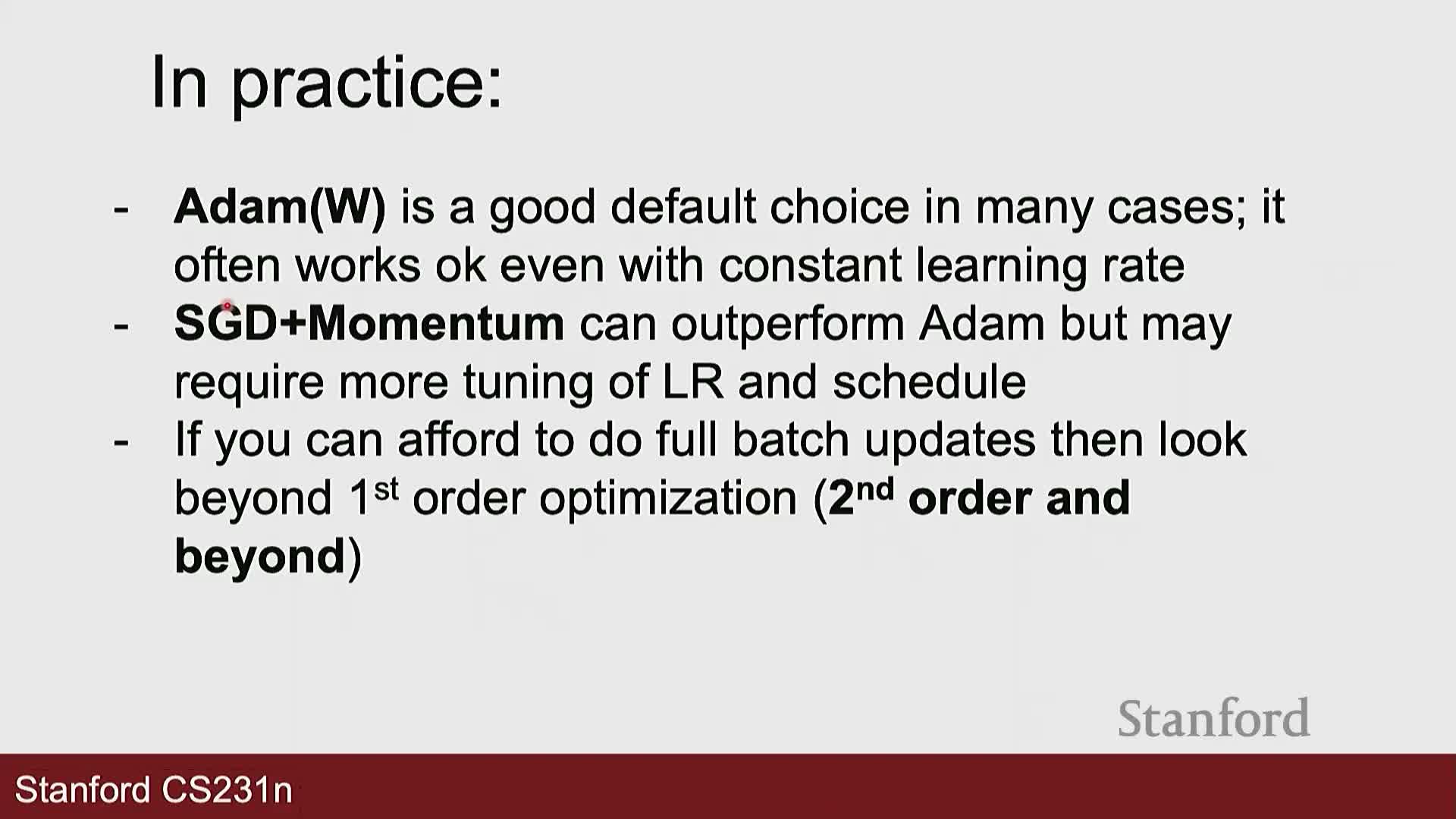
Practical rule of thumb for training new models:
- Start with Adam or AdamW with a linear warm-up followed by cosine decay as an effective default.
- Use SGD with momentum as a competitive alternative when you can invest in careful tuning.
- Reserve second-order approaches for small, full-batch settings; otherwise rely on first-order optimizers with appropriate regularization and learning rate schedules.
- Validate hyperparameters on held-out data and use multiple random seeds to detect instability.
Next topic: optimization and training of nonlinear neural networks (e.g., two-layer networks with activation functions) which extend linear models by inserting elementwise nonlinearities and additional weight matrices to represent more expressive function classes.
Enjoy Reading This Article?
Here are some more articles you might like to read next: