Stanford CS231N | Spring 2025 | Lecture 4- Neural Networks and Backpropagation
- Lecture scope: neural networks and backpropagation as foundational methods
- Review of loss functions: softmax, hinge loss, and scoring
- Gradient-based optimization: gradients, gradient descent, mini-batches, and advanced optimizers
- From linear classifiers to multi-layer networks: dimensions, layers, and hidden units
- Role of nonlinearities and activation functions in expressivity
- Activation selection and hyperparameter practice
- Practical two-layer network implementation and the centrality of analytic gradients
- Model capacity, templates, and regularization versus network size
- Biological inspiration and limits of brain analogies
- Scoring functions, total loss and the need for derivatives for optimization
- Computational graphs as the structural substrate for automatic differentiation
- Backpropagation on a scalar example (f = (x + y) * z): local gradients, chain rule, upstream/downstream
- Purpose of gradients: parameter updates and intuitive interpretation
- Backpropagation through a composite scalar function (sigmoid of linear combination): numerical example
- Elementary gate patterns and modular forward/backward APIs
- Vector, matrix and tensor backpropagation: Jacobians, sparsity and memory considerations
- Efficient matrix-multiply backward formulas and practical implementation patterns
Lecture scope: neural networks and backpropagation as foundational methods
This lecture introduces neural networks and backpropagation as the core mathematical and algorithmic mechanisms that enable layered models to learn from data by computing gradients of a loss with respect to parameters.
-
Backpropagation is presented as the general procedure used across modern learning algorithms to propagate error derivatives from outputs back to parameters in multi-layer architectures.
- This propagation enables gradient-based optimization via variants of gradient descent.
- Understanding these ideas is framed as essential for subsequent topics and practical model development.
Review of loss functions: softmax, hinge loss, and scoring
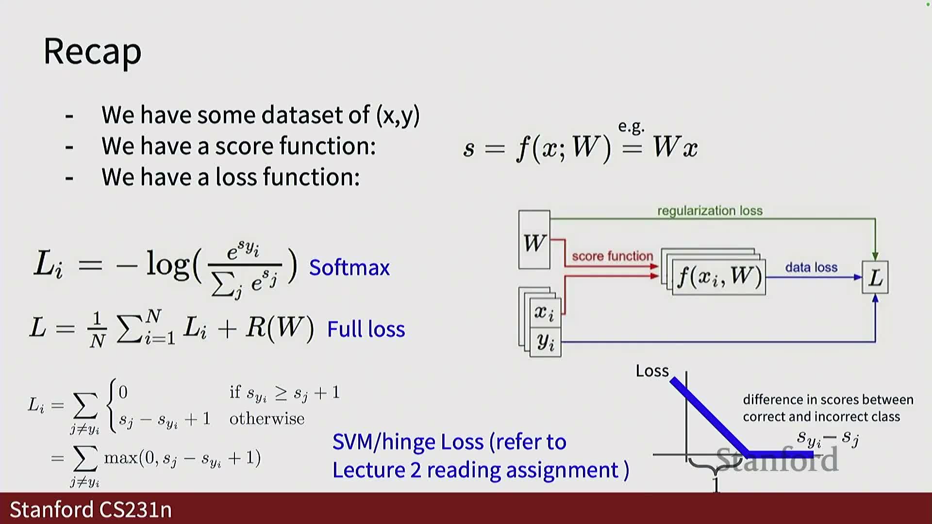
Loss functions convert model scores into scalar objectives to be minimized during training.
- Common choices:
- Softmax cross-entropy — normalizes scores into probabilities and optimizes negative log-likelihood; typically used for probabilistic multiclass classification.
-
Hinge (SVM) loss — enforces margin-based separation without producing probabilities; penalizes cases where the true class score is not larger than competing class scores by at least a margin (often 1). It yields zero loss when the margin constraint is satisfied and increases linearly otherwise.
- Losses are commonly combined with parameter regularization to form the total objective:
-
L = data_loss + lambda * regularizer(W), where lambda scales the regularization penalty.
-
L = data_loss + lambda * regularizer(W), where lambda scales the regularization penalty.
- The choice of loss depends on task requirements and empirical performance.
Gradient-based optimization: gradients, gradient descent, mini-batches, and advanced optimizers
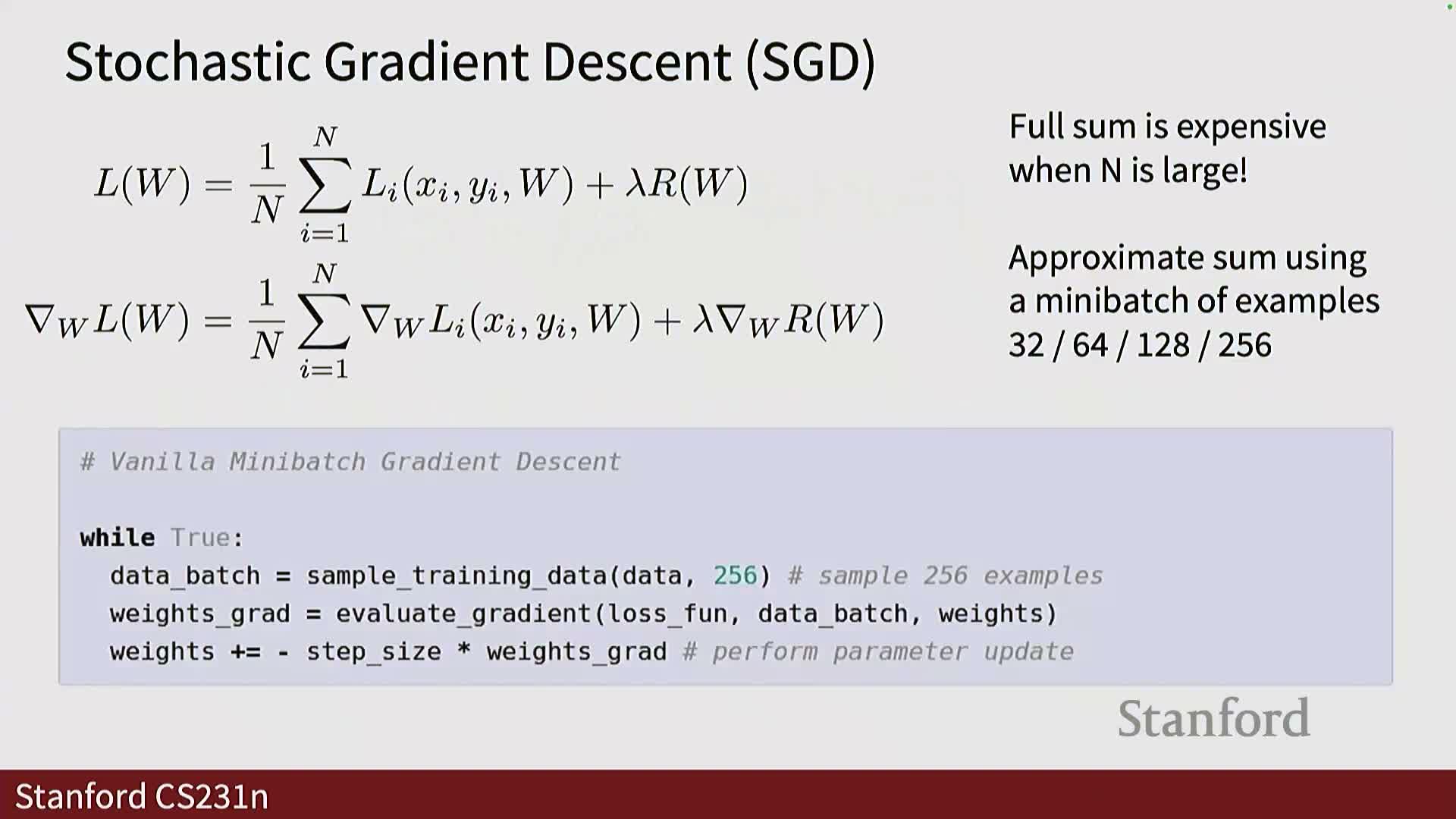
Model parameters are found by minimizing the loss landscape using gradients ∂L/∂W.
- Compute gradient and update parameters in the negative gradient direction scaled by a learning rate (gradient descent): W ← W − η ∂L/∂W.
- For large datasets, computing gradients on the full dataset is often infeasible, so use stochastic gradient descent (SGD) with mini-batches (typical sizes: 32, 64, 128, 256) to approximate the true gradient and update iteratively.
- Practical optimizers extend SGD:
-
Momentum, RMSProp, Adam, and variants accelerate convergence and adapt step sizes.
-
Momentum, RMSProp, Adam, and variants accelerate convergence and adapt step sizes.
-
Learning rate scheduling (decay, step reductions) remains important, although some adaptive optimizers partially encode step-size adaptation internally.
From linear classifiers to multi-layer networks: dimensions, layers, and hidden units
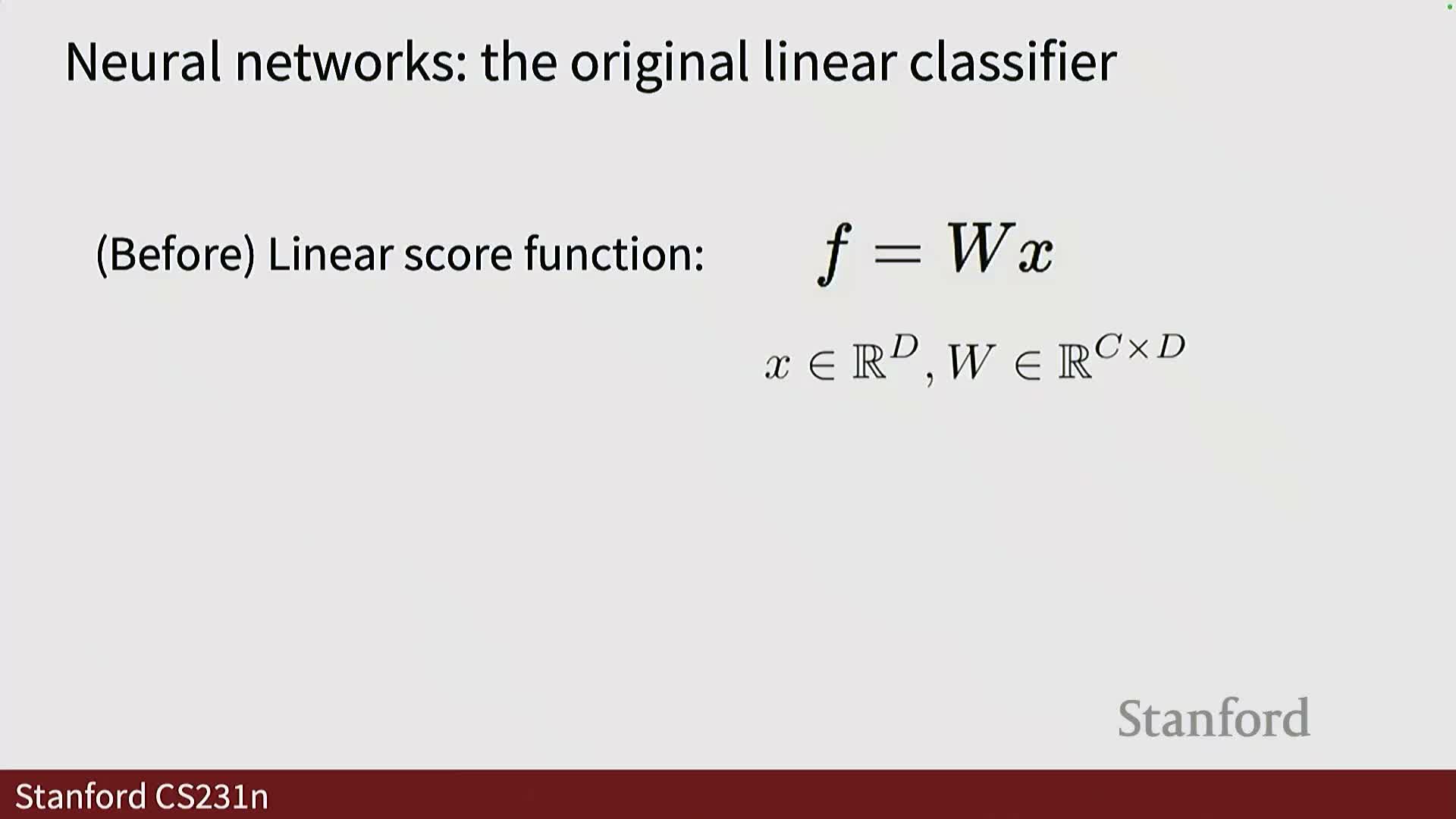
A single-layer linear classifier computes scores s = W x (plus bias), mapping D-dimensional inputs to C outputs — the simplest neural model.
-
Multi-layer networks add one or more hidden layers with H units and additional weight matrices (e.g., W1, W2) so intermediate representations can be learned.
- Maintain dimensional consistency across layers (input dimension D, hidden H, output C).
- Adding layers increases representational capacity by enabling successive linear transformations followed by nonlinearities, mapping inputs into spaces where classes can be linearly separated.
Role of nonlinearities and activation functions in expressivity
Activation functions insert nonlinearity between linear layers so stacked layers cannot be collapsed into a single linear mapping — this nonlinearity is essential to learn complex, nonlinearly separable functions.
- Common activations and tradeoffs:
- ReLU (rectified linear unit, max(0,x)): computationally efficient, mitigates vanishing gradients for positive regimes, but can suffer dead neurons.
- Leaky ReLU / ELU: address zero-region issues by allowing a small gradient when x < 0.
- Swish and variants: used in recent architectures with competitive empirical performance.
-
Sigmoid / Tanh: squash values and can cause vanishing gradients, so they are often reserved for final layers or specialized use.
- Activation choice is a hyperparameter often selected empirically or by following architecture conventions, considering differentiability, zero-centeredness, gradient dynamics, and convergence speed.
Activation selection and hyperparameter practice
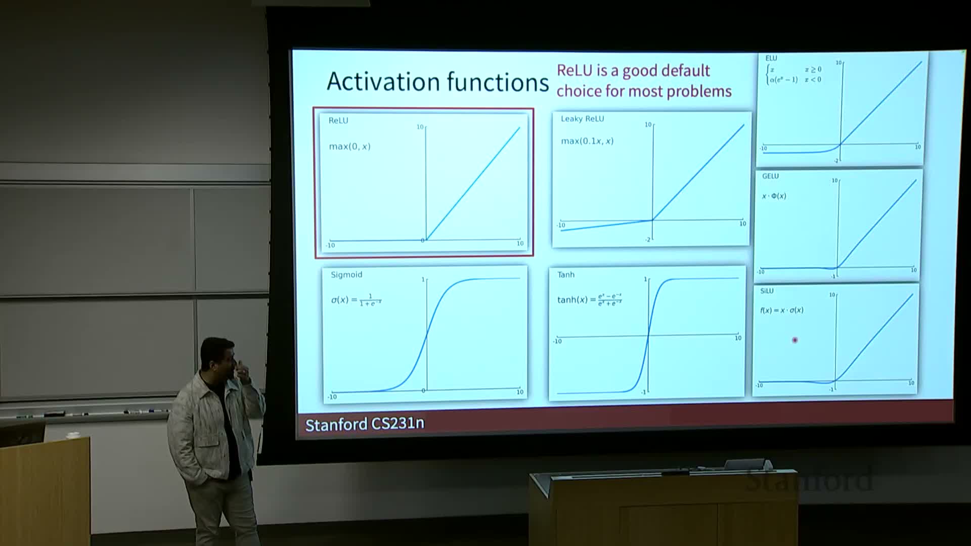
Choosing activation functions and other architectural hyperparameters is largely empirical and problem-dependent.
- Practitioners typically begin with well-tested defaults (e.g., ReLU for CNNs) and explore alternatives when necessary.
- Key desiderata:
- Preserve gradient flow (avoid vanishing gradients).
- Suitable zero-centering.
-
Computational efficiency and training stability.
- Research offers theoretical and empirical guidance, but practical selection often relies on prior work for similar tasks and iterative hyperparameter tuning.
Practical two-layer network implementation and the centrality of analytic gradients
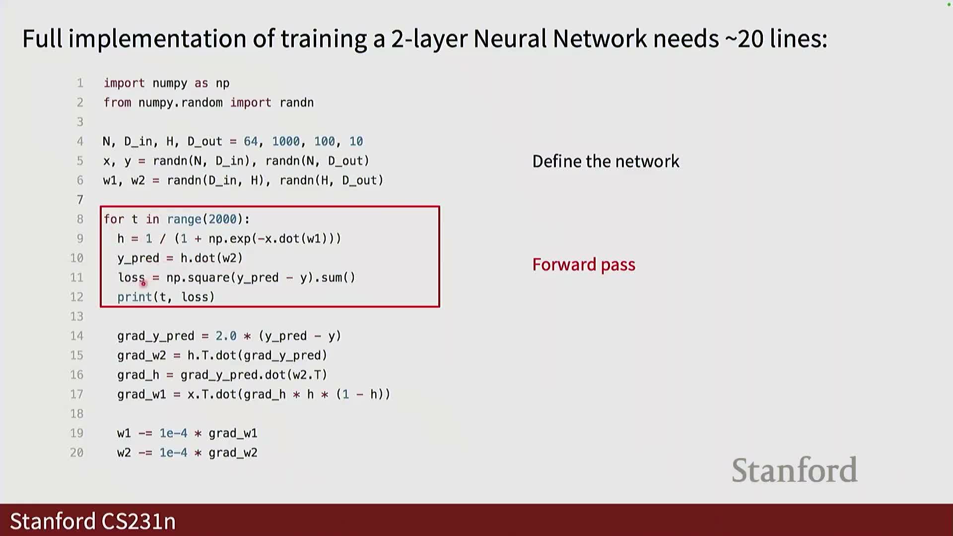
Implementing a two-layer neural network in a high-level language typically involves these steps:
- Define input/output dimensions and hidden layer size.
- Initialize weight matrices and biases.
- Perform a forward pass to compute intermediate representations, scores, and the loss.
- Compute gradients for an optimization step (backward pass).
- Optionally perform numerical gradient checking to validate correctness.
- In practice, analytical gradients (derived by hand or via automatic differentiation) are used for efficiency and numerical stability.
- The bulk of engineering effort is often in correctly formulating and implementing the backward pass to compute ∂L/∂W for all trainable parameters.
- In practice, analytical gradients (derived by hand or via automatic differentiation) are used for efficiency and numerical stability.
Model capacity, templates, and regularization versus network size
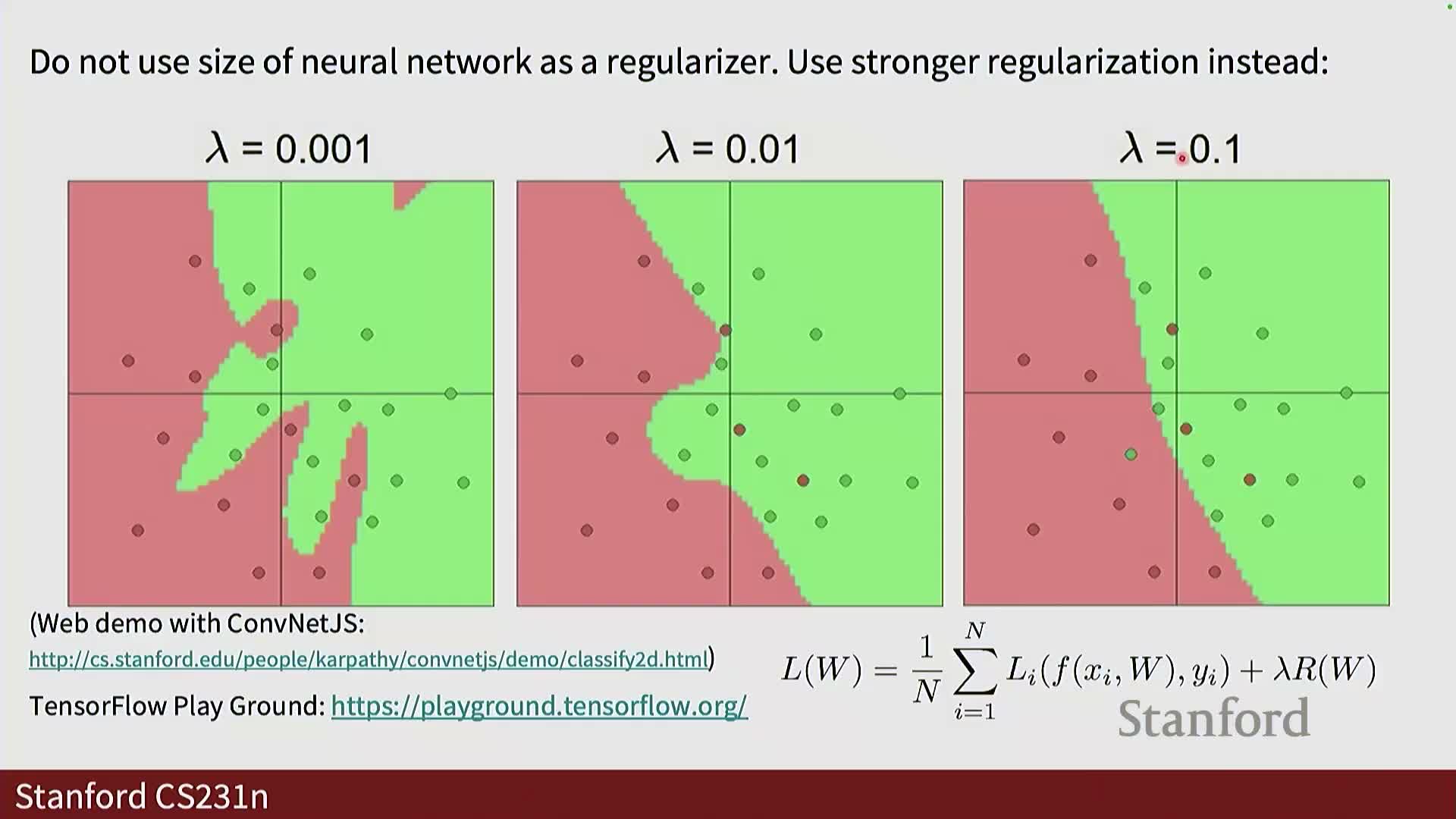
Increasing the number of hidden units increases model capacity, enabling the network to learn more complex decision boundaries and part-based templates (e.g., shared object parts across classes).
- Excessive capacity can lead to overfitting; regularization constrains parameters:
- Common techniques: weight decay, dropout, etc.
- Common techniques: weight decay, dropout, etc.
- The regularization coefficient lambda scales the penalty on weights:
- Too large lambda → underfitting (overly constrained weights).
- Too small lambda → overfitting (memorization).
- The trade-off between capacity and regularization is typically tuned empirically.
Biological inspiration and limits of brain analogies
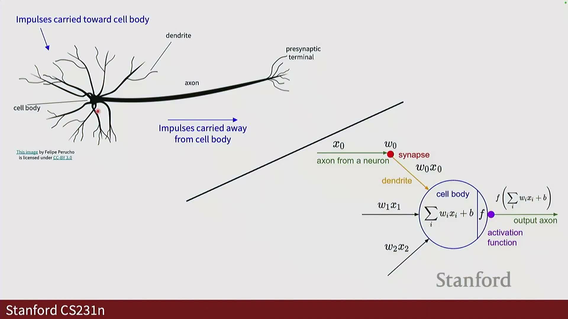
Artificial neural networks borrow high-level metaphors from biological neurons (inputs aggregated by a cell body and transmitted via axons), but these analogies are loose and should not be overinterpreted.
-
Computational neurons implement mathematical functions (weighted sums and activations) for efficiency and simplicity.
- Biological neural dynamics are far more complex; architecture design prioritizes implementation efficiency, scalability, and empirical performance rather than biological fidelity.
Scoring functions, total loss and the need for derivatives for optimization
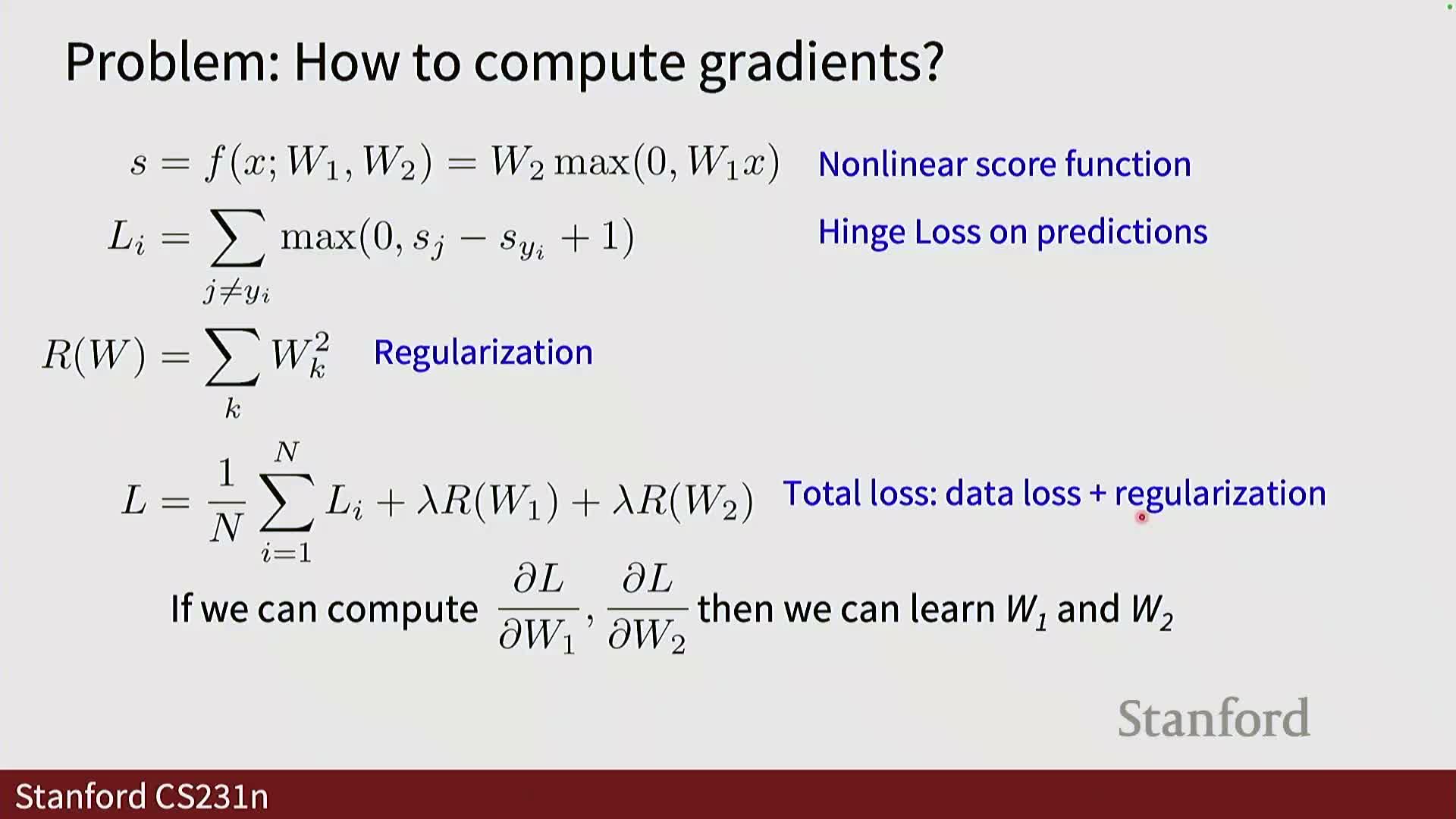
A model maps inputs through weights to produce scores, which are passed to a loss function (e.g., softmax cross-entropy or hinge) and combined with regularizers to form the total objective L(W).
- Optimization requires computing partial derivatives ∂L/∂W for all parameters.
- Deriving these derivatives algebraically for complex models by hand is error-prone and impractical for large architectures or custom losses, motivating systematic computational frameworks for automated derivative computation.
Computational graphs as the structural substrate for automatic differentiation
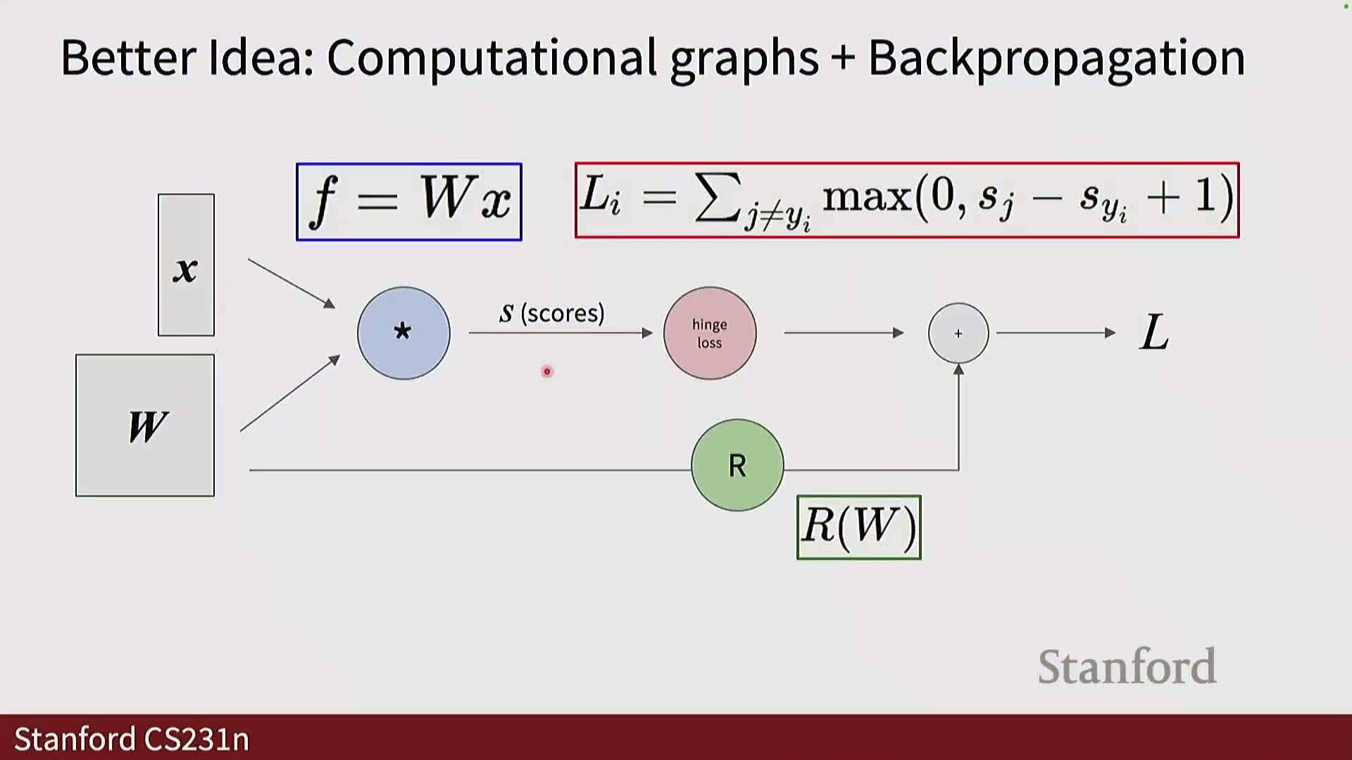
A computational graph represents a model as a directed acyclic graph (DAG) of elementary operations mapping inputs and parameters to the loss output.
- Constructing this graph explicitly enables:
- Local forward computations at each node.
- Systematic backward propagation of gradients via the chain rule.
- Each node exposes a local Jacobian (or local gradient rule), receives an upstream gradient from successors, multiplies them to yield downstream gradients for predecessors, and thus implements reverse-mode automatic differentiation efficiently and modularly.
Backpropagation on a scalar example (f = (x + y) * z): local gradients, chain rule, upstream/downstream
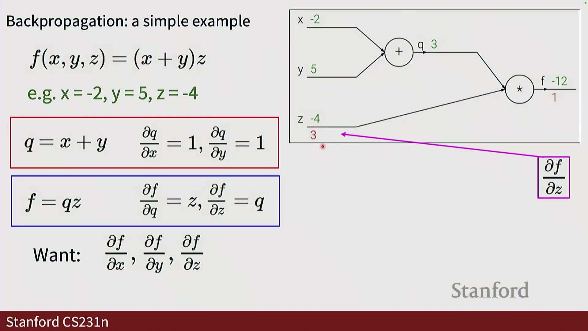
For the scalar function f(x,y,z) = (x + y) * z, forward evaluation and backpropagation proceed as follows:
- Forward pass:
- Compute Q = x + y.
- Compute f = Q * z.
- Local derivatives:
- ∂Q/∂x = 1, ∂Q/∂y = 1.
- ∂f/∂Q = z, ∂f/∂z = Q.
- Backpropagation:
- Start with upstream gradient ∂f/∂f = 1.
- Multiply the upstream gradient by each node’s local gradient to produce downstream gradients.
- This modular multiply-and-propagate yields ∂f/∂x, ∂f/∂y, and ∂f/∂z without computing a global closed-form derivative.
Purpose of gradients: parameter updates and intuitive interpretation
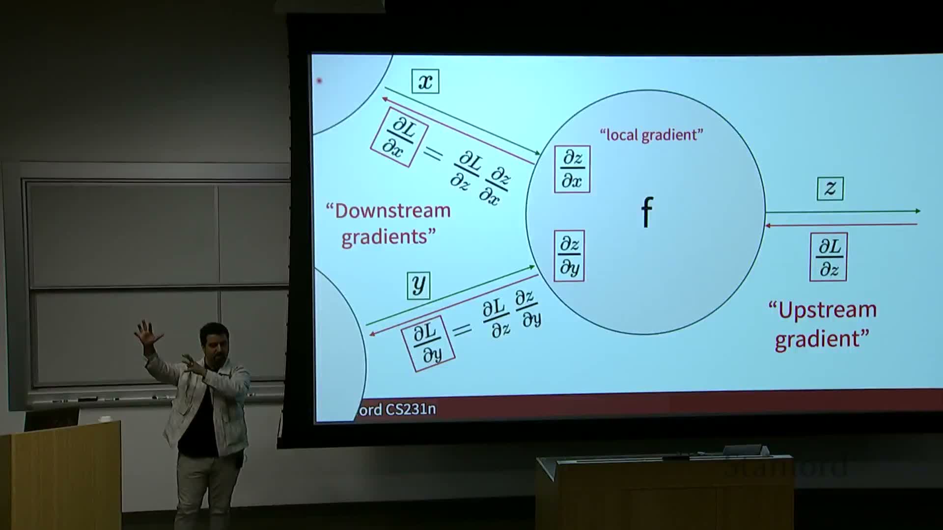
Gradients of the loss with respect to parameters indicate sensitivity: ∂L/∂W quantifies how a small change in a parameter affects the loss.
- Update rule (gradient descent): W ← W − η ∂L/∂W, where η is the learning rate.
-
Backpropagation efficiently computes these sensitivities for every parameter in a multi-layer network by propagating gradients from the loss to each parameter.
- Intuition: gradients point in the direction in parameter space that increases loss, so negative gradients provide the descent direction for optimization.
Backpropagation through a composite scalar function (sigmoid of linear combination): numerical example
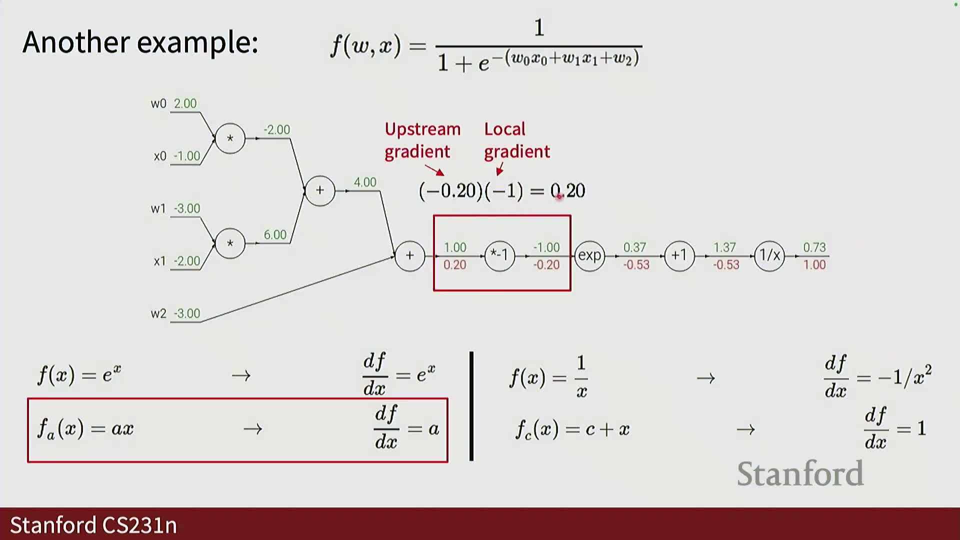
A sigmoid applied to a linear combination implements σ(a) with a = w0 x0 + w1 x1 + ….
- Forward propagation evaluates linear sums, exponentials, and division to produce the output σ(a).
- Backward propagation uses the convenient local gradient:
-
σ’(a) = σ(a) (1 − σ(a)).
-
σ’(a) = σ(a) (1 − σ(a)).
- Backpropagating through a sigmoid requires only the sigmoid value and the upstream gradient, so chaining local gradients yields parameter gradients such as:
-
∂L/∂w_i = x_i * upstream_grad * σ’(a), enabling parameter updates.
-
∂L/∂w_i = x_i * upstream_grad * σ’(a), enabling parameter updates.
Elementary gate patterns and modular forward/backward APIs
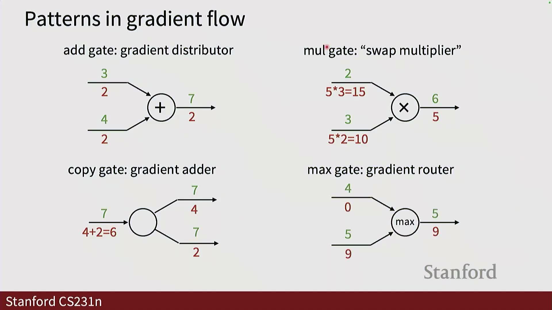
Common computation gates exhibit simple, reusable backward rules that make modular automatic differentiation practical:
-
Add gate: distributes upstream gradients unchanged to inputs.
-
Multiply gate: swaps variables in the gradient (∂(xy)/∂x = y).
-
Copy gate: duplicates gradients to multiple consumers.
-
Max / ReLU gate: routes gradient only to the winning input (the input that achieved the max).
- These local rules support implementing modular forward() and backward() APIs for each operator, storing necessary inputs during the forward pass and encapsulating local backward computations — the design pattern used by deep learning libraries.
Vector, matrix and tensor backpropagation: Jacobians, sparsity and memory considerations
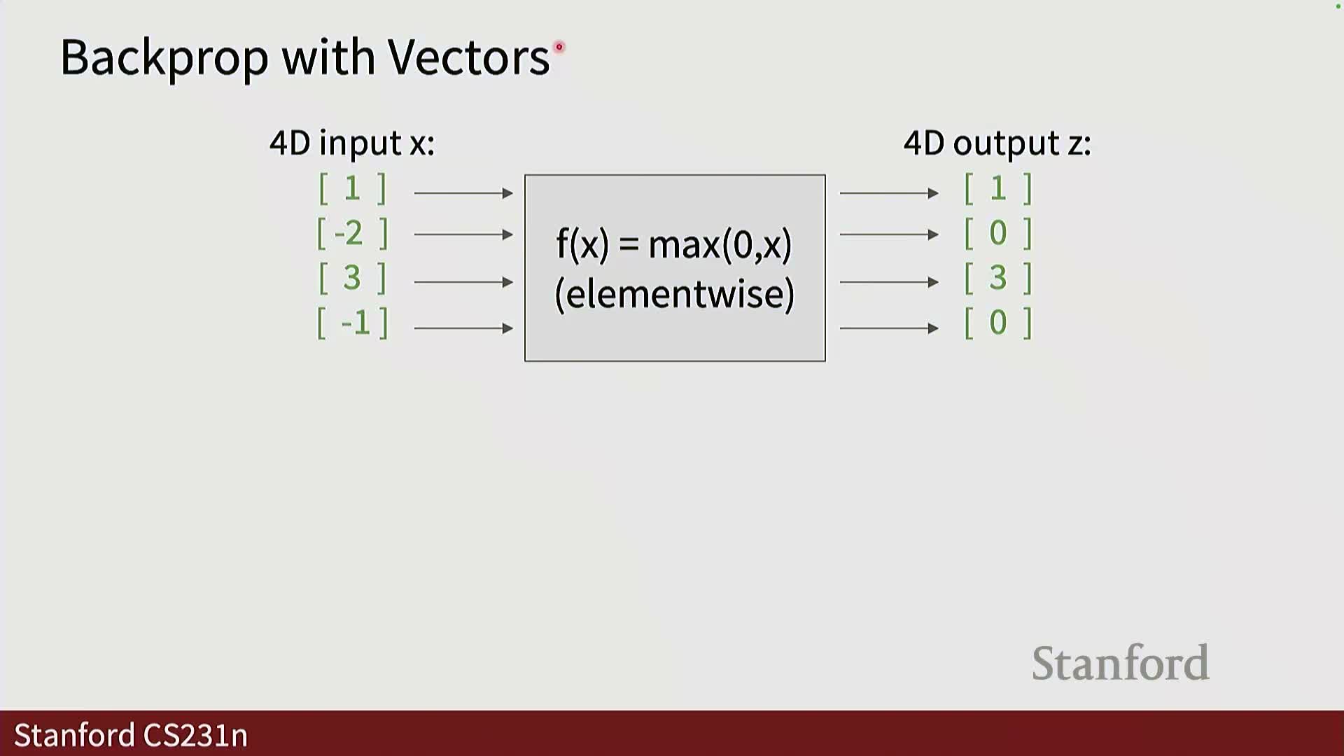
Extending backpropagation to vectors and tensors generalizes scalar derivatives to Jacobians and higher-order derivative tensors.
- When outputs are vectors, local gradients with respect to inputs are matrices whose multiplication with upstream gradient vectors yields downstream gradients with matching input shape.
- Naive Jacobian construction is often infeasible (Jacobian sizes can exceed memory), but many operations are structured so backward rules can be implemented with efficient matrix operations and broadcasting rather than materializing full Jacobians:
- For elementwise ops like ReLU the Jacobian is diagonal (sparse).
- For matrix multiply the backward pass can be implemented via other matrix multiplies (avoiding explicit large Jacobians).
Efficient matrix-multiply backward formulas and practical implementation patterns
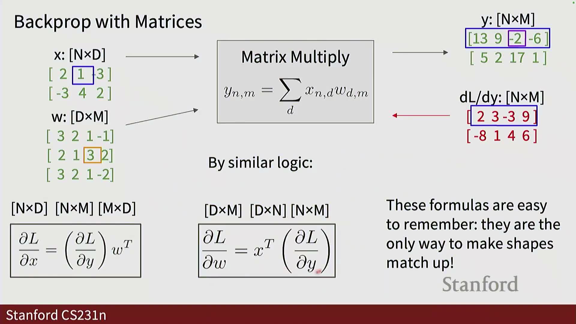
For Y = X W (batch X of shape [N, D], W of shape [D, M], Y of shape [N, M]), the backward pass uses matrix identities:
-
∂L/∂X = ∂L/∂Y · W^T
-
∂L/∂W = X^T · ∂L/∂Y
- These formulas implement the ‘swap’ property of multiplication and avoid forming the full Jacobian of size (NM) × (ND).
- Leveraging these matrix identities enables scalable training with common mini-batch sizes and feature dimensions, and forms the basis for efficient implementations in numerical libraries and deep learning frameworks.
Enjoy Reading This Article?
Here are some more articles you might like to read next: