Stanford CS231N | Spring 2025 | Lecture 5- Image Classification with CNNs
- Instructor introduction and course context
- Recap of deep learning fundamentals: problem formulation, linear classifiers, losses, and optimization
- From linear classifiers to neural networks; computational graphs and backpropagation
- General recipe for deep learning and transition to vision-specific models
- Hand-designed feature representations vs end-to-end learned representations
- Architectural design tradeoffs for image models; introduction to convolutional networks
- Historical evolution: early CNNs, AlexNet, and the rise of transformers
- Lecture roadmap and the convolution/pooling primitives
- Fully connected layers as global template matchers and the motivation for local filters
- Convolutional layer mechanics, filters, biases, parameters, and batching
- Stacking convolutions, representational power and the need for nonlinearities
- Visualization of learned filters and higher-layer receptive patterns
- Spatial dimension arithmetic: output size formula, padding, and same padding
- Parameter counts and computational cost (FLOPs) for convolutions
- Convolution variants and brief introduction to pooling
- Downsampling strategies, batching, aspect ratio handling, and translation equivariance
- Summary and next steps: assembling CNN architectures
Instructor introduction and course context
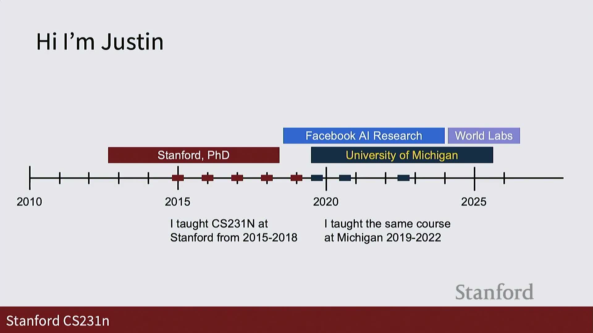
Instructor introduction: the instructor’s background is in deep learning, with teaching experience and recent activity in both industry and academia—this lecture is positioned at the start of the course segment on visual perception.
The passage situates the lecture in the course timeline: prior lectures covered foundational deep learning material, and the course now transitions toward more specialized topics in vision.
This orientation clarifies that subsequent technical content should be read as an applied specialization of earlier, general deep learning recipes—preparing the reader to connect general methods to image-specific design choices.
Recap of deep learning fundamentals: problem formulation, linear classifiers, losses, and optimization
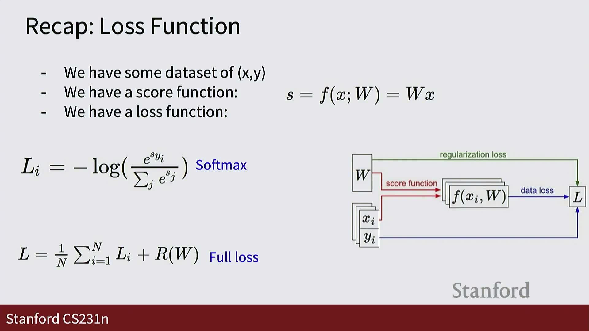
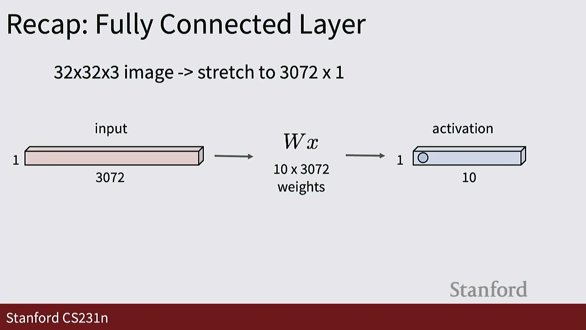
Deep learning problems are expressed as mappings between input and output tensors: for images, inputs are three-dimensional grids of pixels (height × width × channels) and outputs are class score tensors.
- A linear classifier implements a simple functional form f(x) = W x, producing a score per category.
- Candidate weight matrices are evaluated by loss functions such as softmax cross-entropy or SVM loss.
-
Optimization algorithms (stochastic gradient descent variants including momentum, RMSProp, and Adam) traverse parameter space to minimize the chosen loss, and optimizer research (e.g., recognition for Adam) remains central to practical training.
This set of choices—problem encoding, model parameterization, loss definition, and gradient-based optimization—is the core pipeline for training models.
From linear classifiers to neural networks; computational graphs and backpropagation
Linear classifiers are limited: they compress category structure into single global templates and separate data with hyperplanes, which fails when classes are not linearly separable or exhibit diverse appearances.
Neural networks generalize linear classifiers by stacking linear maps with elementwise nonlinearities, yielding far richer function classes while retaining the same optimization target: minimize a loss over parameters.
-
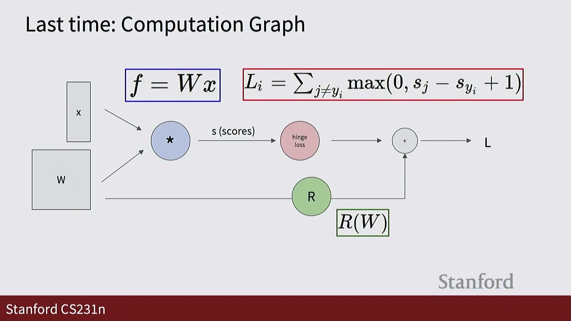
Computational graphs organize neural computation as primitive nodes (matrix multiplies, nonlinearities, etc.).
- A forward pass computes outputs from inputs.
- A backward pass computes gradients using the chain rule.
- A forward pass computes outputs from inputs.
-
Backpropagation reduces global gradient computation to local gradient computations per node, enabling automatic differentiation through arbitrarily complex architectures and powering end-to-end gradient-based learning.
General recipe for deep learning and transition to vision-specific models
The general deep learning recipe is:
- Represent inputs and outputs as tensors.
- Construct a computational graph that maps inputs to outputs.
- Define a loss for the target task.
- Optimize the graph parameters with gradient descent via backpropagation.
This recipe is task-agnostic and applies across modalities (images, audio, text).
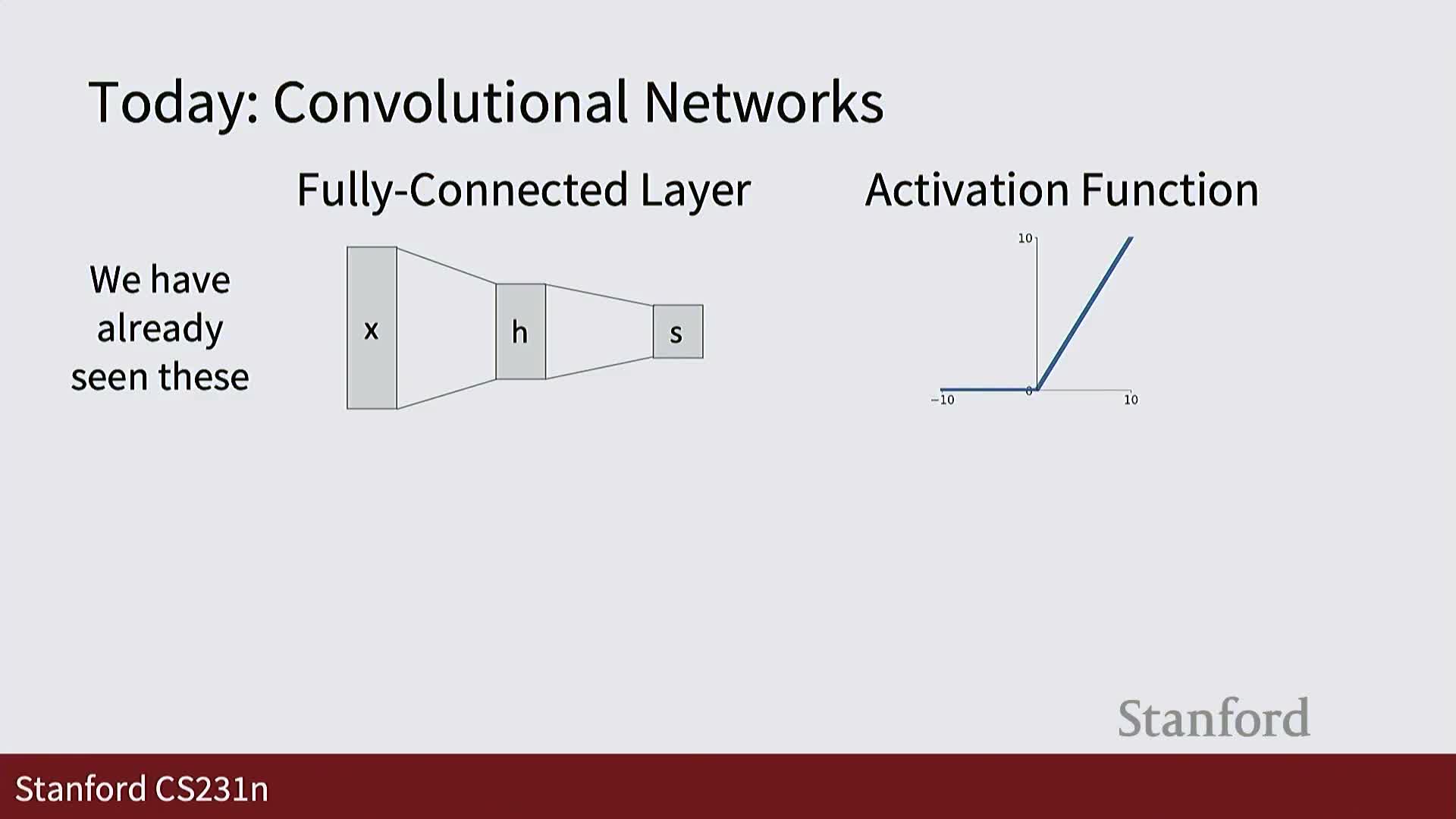
For images, architectures that respect 2D spatial structure outperform naive vectorized fully connected networks—motivating the introduction of convolutional networks, which incorporate operators tailored to spatially structured data.
Hand-designed feature representations vs end-to-end learned representations
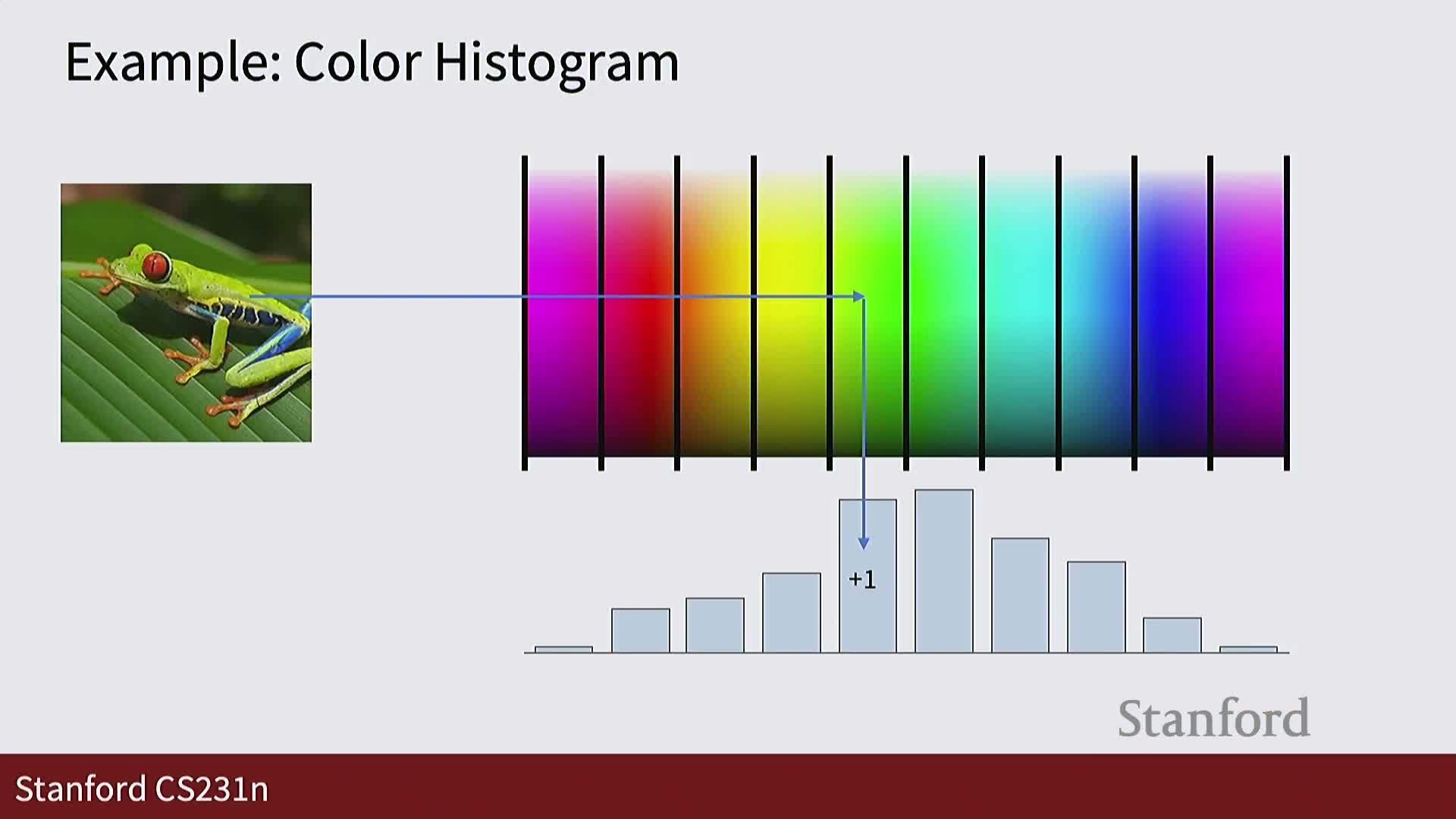
Before deep learning, image systems used hand-engineered feature extractors (e.g., color histograms, HOG, concatenations of multiple features) to convert pixel grids into compact vectors for downstream classifiers.
- These pipelines remove or transform spatial information according to human priors, then train a simple classifier on top.
-
End-to-end learning lets gradient descent tune all model components from raw pixels to final outputs, replacing fixed handcrafted feature functions with a learnable family of functions defined by network architecture.
The conceptual difference is which parts are fixed by designers (feature extractor) versus learned from data (network weights). Empirical evidence over the last decade favors learning representations end to end for many vision tasks when large datasets and compute are available.
Architectural design tradeoffs for image models; introduction to convolutional networks
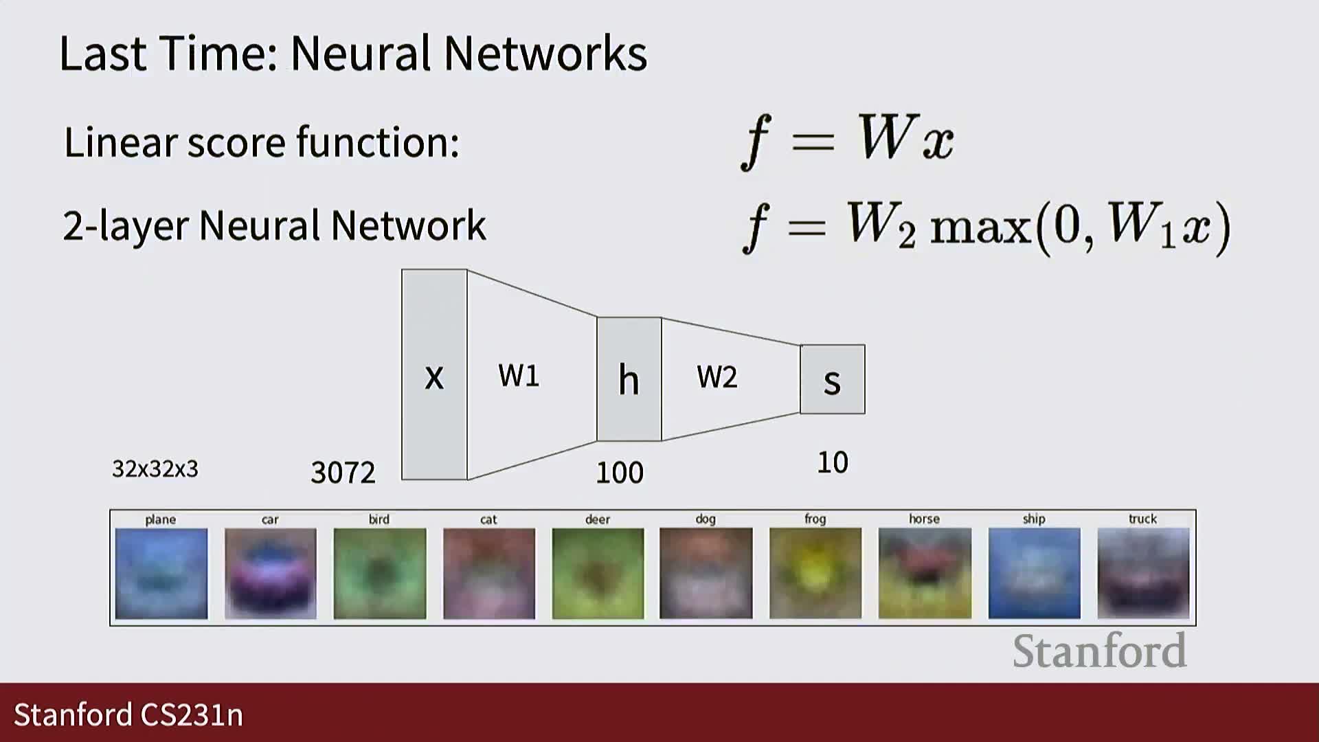
Designing neural networks for images means specifying a family of functions via a computational graph that preserves useful inductive biases rather than hand-coding a single feature extractor.
-
Convolutional neural networks (CNNs) embed spatially aware primitives—convolutional layers and pooling—so that learned functions respect local structure and translation-related invariances.
- A typical CNN comprises:
- A body of interleaved convolution, nonlinearity, and pooling layers that extract hierarchical features.
- A small fully connected classifier that maps those features to task-specific outputs.
- A body of interleaved convolution, nonlinearity, and pooling layers that extract hierarchical features.
All parameters are learned end to end by minimizing a loss on labeled data. Human design choices remain important at the architecture level (operator sequence, filter counts and sizes), while learning determines specific filters and feature mappings.
Historical evolution: early CNNs, AlexNet, and the rise of transformers
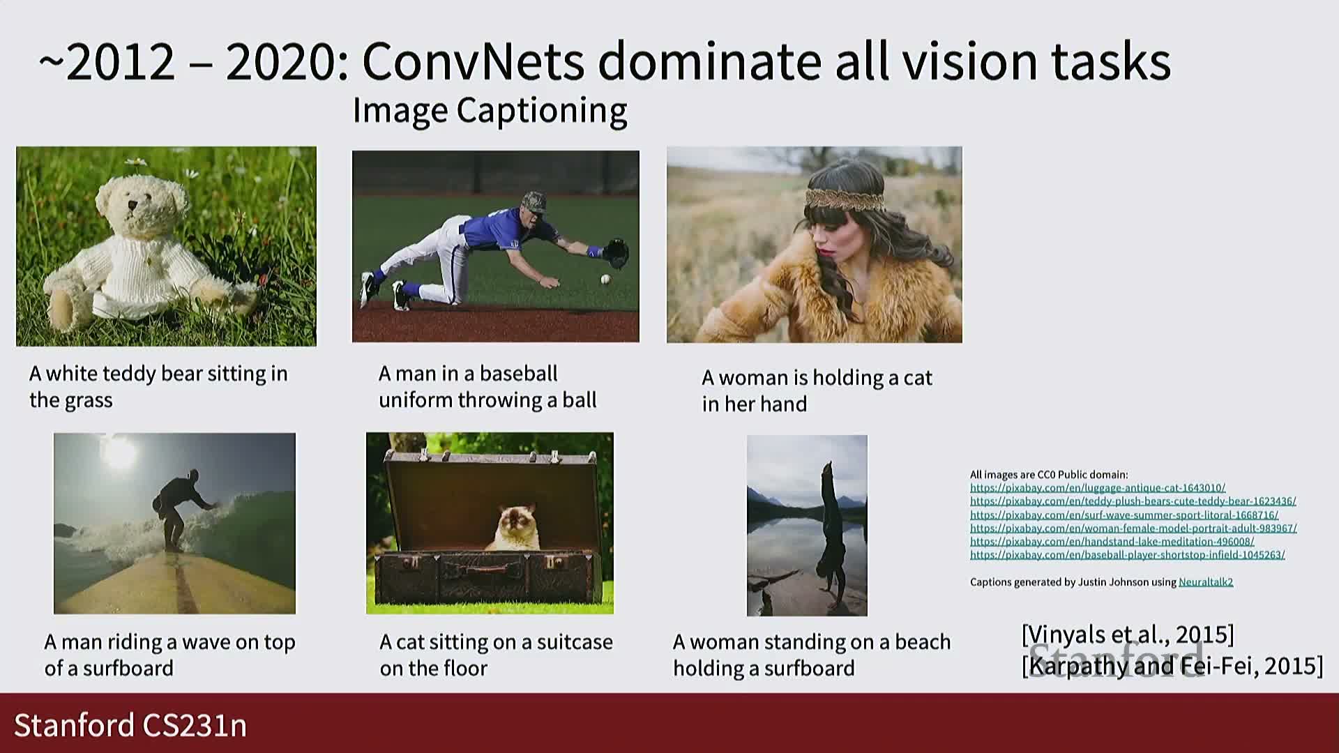
Historical context: convolutional architectures date back decades (e.g., LeNet, 1998) and achieved dramatic practical success starting with AlexNet (2012), driven by larger datasets and GPU acceleration.
- From roughly 2012–2020, CNNs were the default architecture for visual recognition (classification, detection, segmentation, image captioning, early generative models).
- Since 2020–2021, transformer architectures—initially developed for language—have been adapted to images and often match or exceed CNN performance at scale; current practice uses transformers or hybrid CNN-transformer models depending on data and compute tradeoffs.
Why studying convolutions remains valuable:
-
Historical importance and intuition-building.
-
Continued practical use and role in hybrid designs.
Lecture roadmap and the convolution/pooling primitives
Practical CNN construction requires two additional primitive node types beyond dense layers and nonlinearities: the convolutional layer and the pooling layer.
- The convolution layer implements learned local template matching by sliding small multi-channel filters across spatial dimensions to produce activation maps.
- The pooling layer provides an efficient, low-cost mechanism for spatial downsampling.
The lecture aims to define these primitives precisely, explain their hyperparameters (filter size, stride, padding, number of filters), and show how they assemble into convolutional networks that map raw pixel tensors to hierarchical feature representations.
Fully connected layers as global template matchers and the motivation for local filters
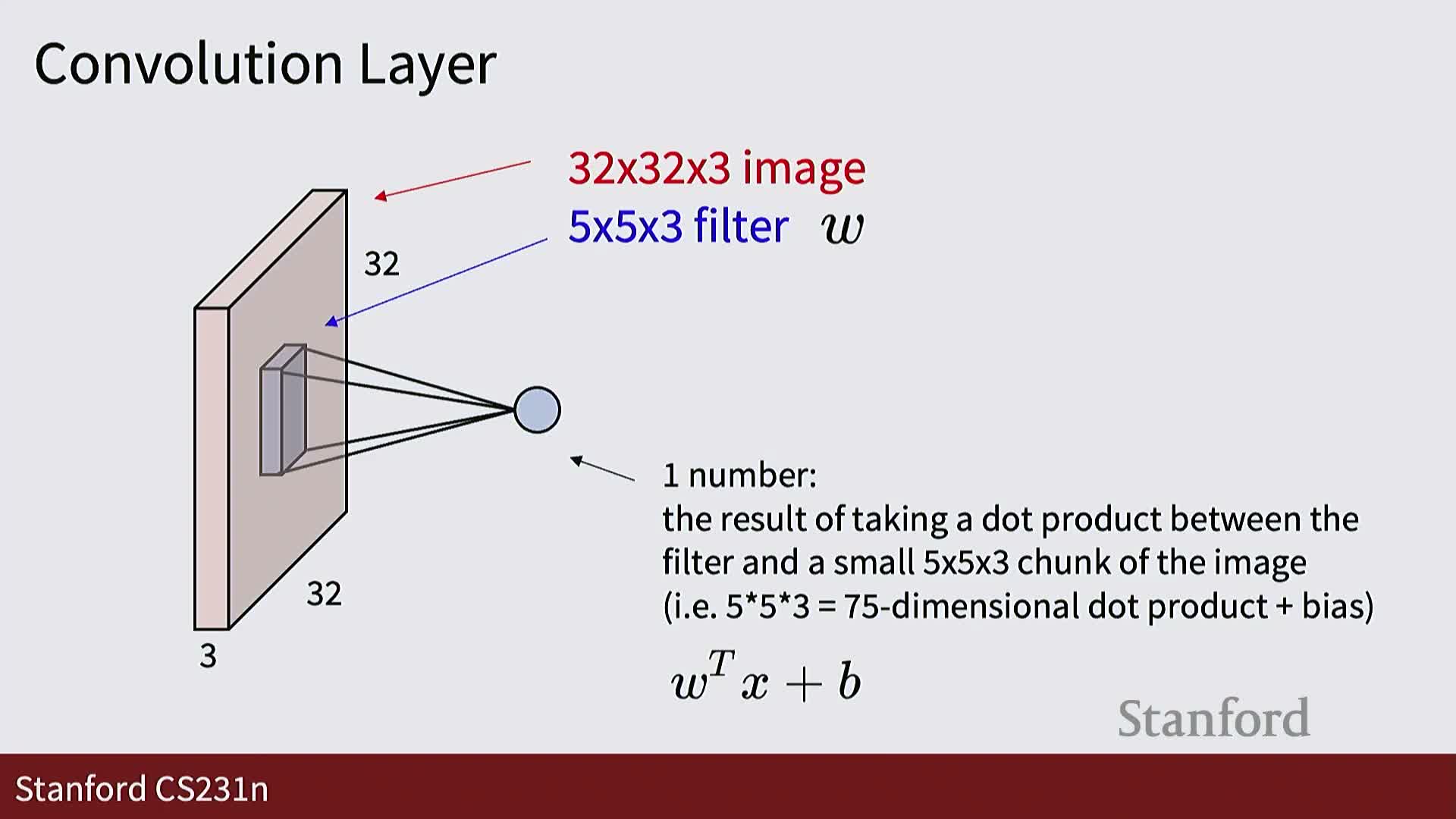
A fully connected (dense) layer computes each output element as the dot product between a learned template (a row of W) and the entire flattened input—acting as a global template matcher over the image.
Convolutional layers generalize this by learning small spatially localized templates (kernels) that span the full channel depth but only a small spatial footprint (e.g., 5×5×C).
- Convolution computes inner products between a kernel and local input patches at every spatial location, producing a spatial response plane per kernel.
- Stacking many kernels yields an output tensor with multiple feature planes that preserve spatial structure.
Key benefits: reduced parameter count, encoded locality priors, and weight sharing across spatial positions—properties crucial for efficient and effective vision models.
Convolutional layer mechanics, filters, biases, parameters, and batching
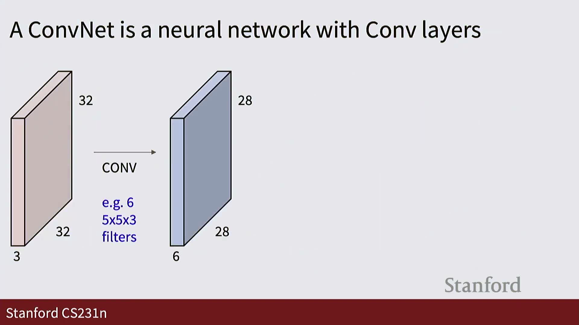
A convolutional layer is parameterized by a filter bank of shape (C_out, C_in, K_h, K_w) where each filter is a small C_in × K_h × K_w tensor convolved across spatial dimensions.
- Sliding a filter over an input volume computes dot products with local patches and yields a 2D activation map per filter.
- Each filter typically has an associated scalar bias added uniformly across its spatial activation map.
- Filter values are learned parameters, initialized randomly to break symmetry so different filters converge to distinct functions.
In practice, convolution is applied to batches of N inputs, yielding N × C_out × H’ × W’ outputs. The typical training loop alternates:
- Forward passes to compute outputs.
- Loss evaluation.
- Backward passes to compute gradients.
- Optimizer steps to update filter parameters.
Hyperparameters (filter count, spatial size, stride) are set prior to training; numeric filter weights and biases are learned parameters.
Stacking convolutions, representational power and the need for nonlinearities
Stacking linear convolutional operators without intermediate nonlinearities results in an overall linear mapping equivalent to a single convolutional operator—so depth alone adds no representational power if layers are linear.
Introducing pointwise nonlinear activation functions (e.g., ReLU and variants) between convolutional layers breaks linearity and yields exponentially more expressive hierarchical feature mappings.
- CNNs therefore interleave convolution and activation layers to build deep function classes that can approximate complex spatial patterns.
- Additional architectural elements (pooling, normalization) further shape feature geometry for downstream tasks.
Architectural design must incorporate nonlinearities to realize the modeling benefits of depth.
Visualization of learned filters and higher-layer receptive patterns
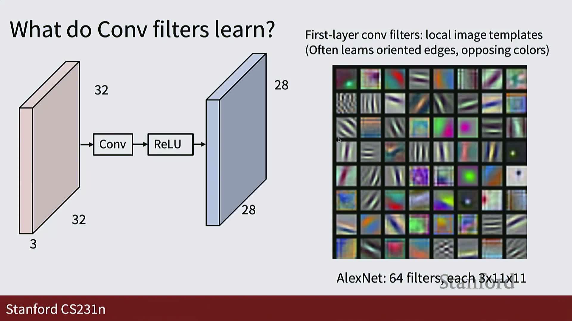
First-layer convolutional filters trained on natural images typically resemble edge detectors and color-opponency blobs—small localized RGB patches sensitive to colors and oriented gradients—because these basis functions efficiently capture low-level image statistics.
- Higher-layer filters respond to progressively larger and more abstract spatial structures: motifs like eyes, wheels, text, or object parts.
- These emergent representations arise automatically from random initialization plus gradient-based optimization; symmetry breaking in initialization is essential so filters do not remain identical.
Visualizing filters and their top-activating image patches provides interpretable insight into hierarchical feature extraction across network depth.
Spatial dimension arithmetic: output size formula, padding, and same padding
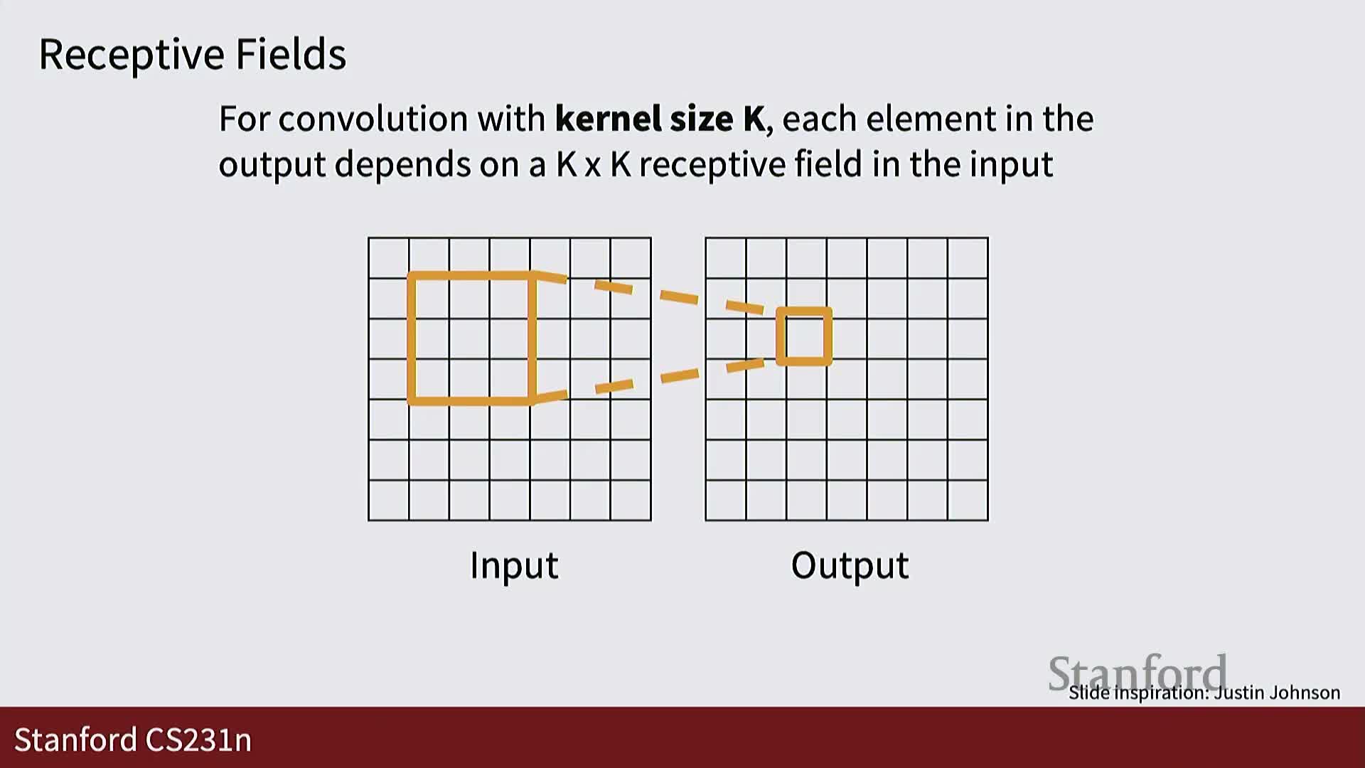
The spatial output size of a convolution over input width W with kernel size K and no padding is W’ = W − K + 1, because the kernel can be placed at each valid starting location.
With padding P zeros around the input the formula becomes W’ = W − K + 1 + 2P.
Choosing odd kernel sizes and setting P = (K − 1) / 2 yields “same” padding, making output spatial dimensions equal input dimensions—this simplifies network design and preserves spatial resolution.
Padding introduces boundary effects (a signal-processing consideration), but same-padding is widely used in practice to maintain spatial layout and simplify stacking layers.
Parameter counts and computational cost (FLOPs) for convolutions
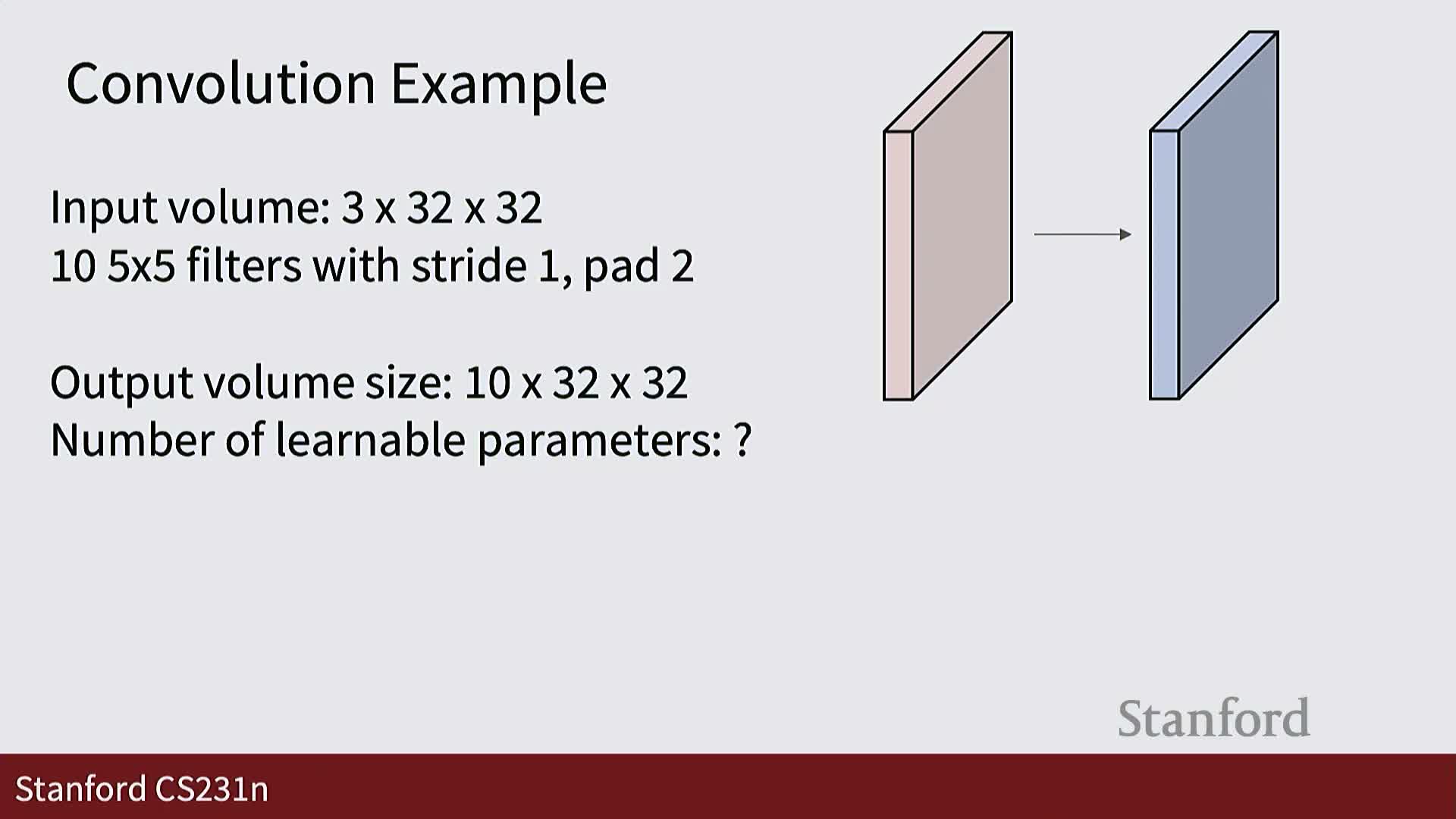
The number of learnable parameters in a convolutional layer equals C_out × (C_in × K_h × K_w) plus C_out biases, reflecting per-filter weight tensors and per-filter biases.
Computational cost (multiply-add FLOPs) is computed by multiplying the number of output elements (N × C_out × H’ × W’) by the kernel element count (C_in × K_h × K_w), since each output element is a dot product between a kernel and an input patch.
Estimating parameter counts and FLOPs per layer is essential for architecture scaling and hardware budgeting because convolutions dominate runtime and memory usage in typical vision networks.
Convolution variants and brief introduction to pooling
Convolution generalizes across input dimensionalities: 1D convolutions operate over sequences, 2D over images, and 3D over volumetric or spatiotemporal signals—using the same local kernel-and-slide mechanics adapted to the relevant axes.
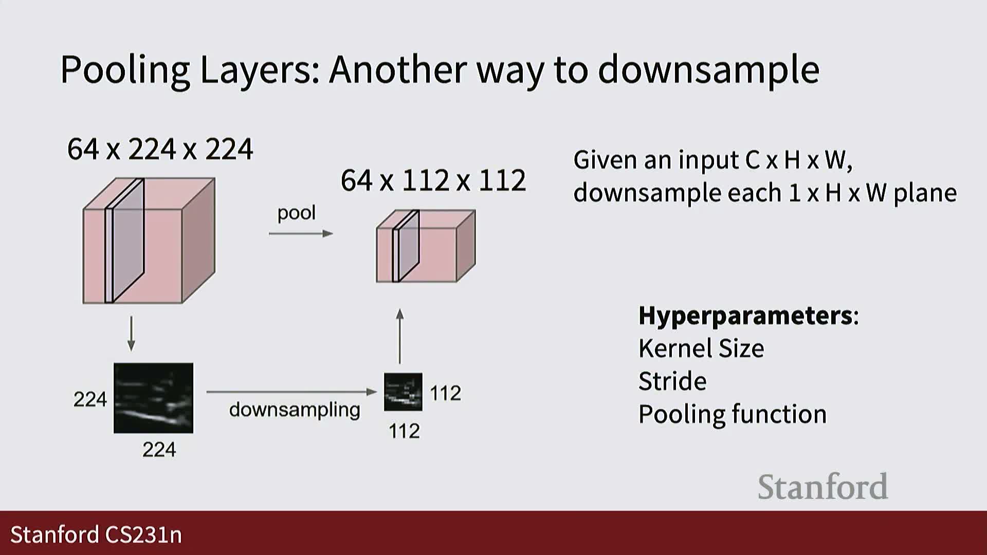
Pooling layers provide a cheap, often nonparametric mechanism to downsample feature maps by partitioning each channel’s spatial domain into local windows and applying a reduction function per window (e.g., max, average, or anti-aliased pooling).
- Pooling preserves channel count while reducing spatial resolution.
- Pooling is typically interleaved with convolutions to reduce spatial size, increase effective receptive field quickly, and lower computational cost compared with repeated strided convolutions.
Downsampling strategies, batching, aspect ratio handling, and translation equivariance
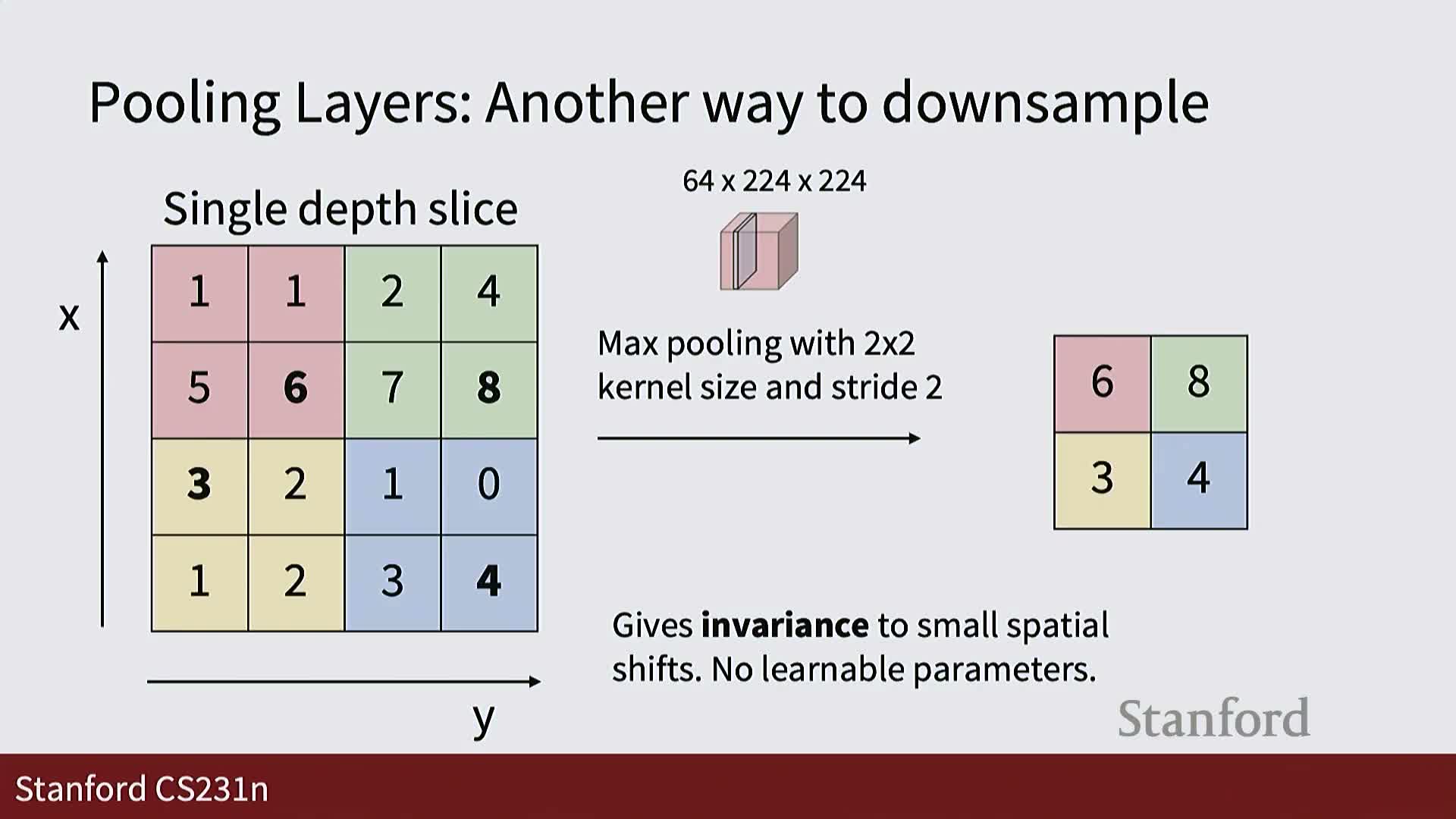
Downsampling in CNNs is commonly implemented via strided convolution or pooling:
-
Max pooling (commonly kernel 2×2, stride 2) is a nonlinear downsampling that selects local maxima.
-
Average pooling is linear and may require a separate nonlinearity elsewhere to introduce nonlinearity into the representation.
Practical systems handle varying input sizes by resizing, zero-padding, or bucketing images by aspect ratio so batched inputs share dimensions—maintaining consistent input sizes per batch is required for standard tensor implementations.
Convolution and pooling are translation-equivariant operators: translating the input and then applying the operator produces the same translated output as applying the operator and then translating the result (modulo boundary handling).
This equivariance and localized weight sharing formalize the inductive biases that make CNNs effective for image data.
Summary and next steps: assembling CNN architectures
Summary: convolutional neural networks combine convolutional layers, nonlinearities, and pooling into hierarchical architectures that process raw pixels to produce task-specific outputs, trained end to end by backpropagation and gradient-based optimization.
Key hyperparameters include filter sizes, number of filters per layer, stride, padding, and pooling configuration—these determine receptive field growth, parameter count, and computational cost, and are typically set by architecture design and cross-validation.
Subsequent design and engineering focus on arranging these primitives into effective topologies (e.g., interleaving conv and pool, then adding fully connected classifiers) and exploring variant modules described in later material. Practitioners should next study concrete CNN architectures and their implementation details.
Enjoy Reading This Article?
Here are some more articles you might like to read next: