• Lecture overview: building and training convolutional neural networks
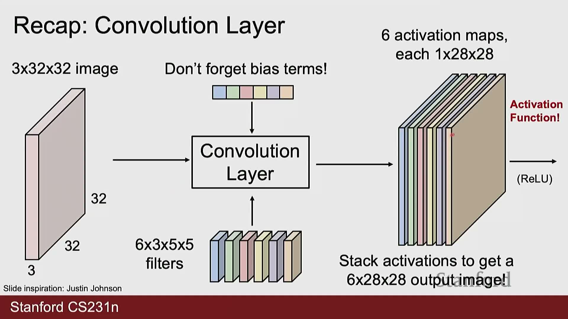
• Convolution layers compute local dot-product responses with multiple learned filters producing activation maps
• Pooling layers reduce spatial resolution while fully connected layers perform global linear mapping followed by activations
• Normalization layers standardize activations to a unit Gaussian and then apply learned scale and shift parameters
• Layer normalization computes per-sample statistics while batch, instance and group norms compute statistics over different subsets
• Dropout regularizes networks by randomly zeroing activations during training and scaling at test time
• Nonlinear activation functions introduce expressivity; ReLU and smooth variants like GELU or CELU mitigate vanishing gradients
• Classic CNN architectures stack convolutional and pooling layers then large fully connected classifiers
• Stacking multiple 3x3 convolutions grows the effective receptive field linearly (three 3x3 layers -> 7x7 receptive field)
• Multiple small convolutions are more parameter-efficient and more expressive than a single large convolution
• Residual connections mitigate optimization problems in very deep networks by enabling residual learning
• ResNet design practices: residual blocks, stage transitions, and scalable model families
• Kaiming (He) initialization preserves activation variance for ReLU networks by scaling by sqrt(2/fan_in)
• Image preprocessing standardizes RGB channels by dataset mean and standard deviation
• Data augmentation increases training diversity and improves generalization by applying label-preserving transformations at train time
• Common image augmentations include horizontal flip, random resized crop, multi-crop test-time augmentation, color jitter, and cutout
• Transfer learning strategies: freeze pretrained features for very small datasets or fine-tune entire networks for larger similar datasets
• Hyperparameter debugging and search: overfit a tiny dataset to validate implementation, then use coarse random search for tuning

Lecture overview: building and training convolutional neural networks

Lecture structure: The lecture is organized into two complementary components:

• (1) Architecture assembly: how to combine convolutional, pooling, normalization, and fully connected building blocks into complete convolutional neural network (CNN) architectures.
  
• (2) End-to-end training: how to train those architectures, including data preparation, augmentation, optimization, and hyperparameter selection.
  

The overview frames the subsequent sections on layer types, activation functions, canonical architectures (e.g., AlexNet, VGG, ResNet), initialization strategies, and practical training recipes for both large-scale and limited-data regimes.

Convolution layers compute local dot-product responses with multiple learned filters producing activation maps

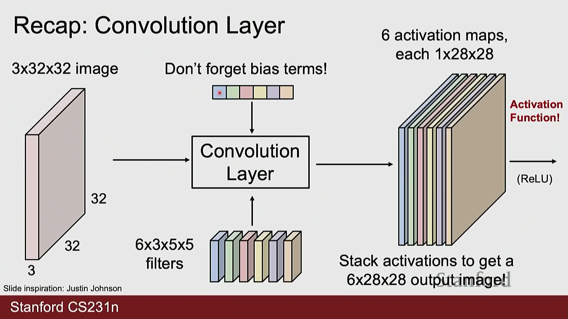
Convolutional layers apply a set of learned filters that match the input depth and slide across spatial locations to compute a dot product plus bias at each position, producing one activation map per filter.

• Each filter spans the full input depth (for example, RGB channels) and is applied at every spatial location according to stride and padding.
  
• The resulting activation maps are typically passed through a pointwise nonlinearity such as ReLU.
  
• When stacking convolutional layers, the next layer’s filters span a depth equal to the number of activation maps produced by the previous layer, enabling hierarchical feature extraction.
  

Pooling layers reduce spatial resolution while fully connected layers perform global linear mapping followed by activations

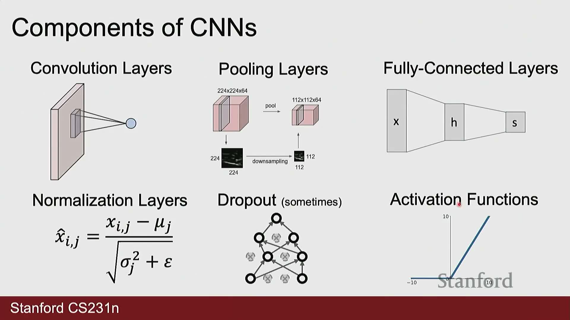
Pooling layers aggregate local spatial neighborhoods to reduce spatial dimensions and computational cost.

• Common choice: 2x2 pooling with stride 2 (max or average).
  
• Pooling reduces height and width while preserving depth, consolidating local information and lowering resolution and compute needs.
  

Fully connected (FC) layers implement a matrix multiply followed by an activation and typically serve as global classifiers or regressors after convolutional feature extraction.

• The final FC layer must output one score per target class (e.g., 1000 for ImageNet).
  

Normalization layers standardize activations to a unit Gaussian and then apply learned scale and shift parameters

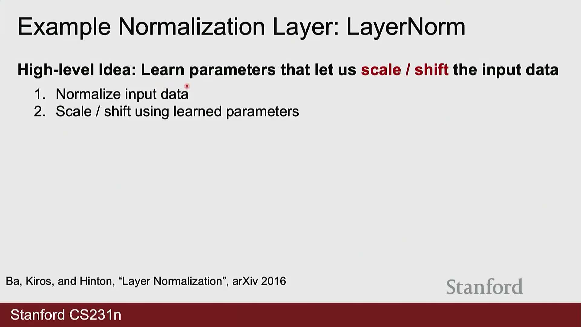
Normalization layers operate in two phases to stabilize activations:

1. Compute mean and standard deviation for a chosen subset of activations.
   
2. Normalize inputs to zero mean and unit variance, then apply learned affine parameters (scale and shift) to the normalized outputs.
   

This procedure conditions optimization by keeping activation statistics well behaved across layers. Different normalization schemes differ only in how they compute the statistics (over batch, over channels, over spatial dimensions, or combinations thereof).

Layer normalization computes per-sample statistics while batch, instance and group norms compute statistics over different subsets

Layer normalization and common variants — all follow the same normalize-then-scale-and-shift pattern but differ where statistics are estimated:

• Layer Normalization: computes mean and variance per sample across all channels and spatial positions (or across the vector dimension for non-convolutional inputs). Then applies learnable scale and shift per sample. Robust to small batch sizes and widely used in transformer models.
  
• Batch Normalization: computes per-channel statistics aggregated across the mini-batch, then applies a per-channel affine transform. Best suited to moderate-to-large batch sizes.
  
• Instance Normalization: computes statistics per-channel per-sample (useful in style transfer and certain generative tasks).
  
• Group Normalization: partitions channels into groups and computes statistics per-group, trading off between layer and instance behaviors.
  

All variants trade off how and where statistics are estimated, which affects robustness to batch size and domain characteristics.

Dropout regularizes networks by randomly zeroing activations during training and scaling at test time

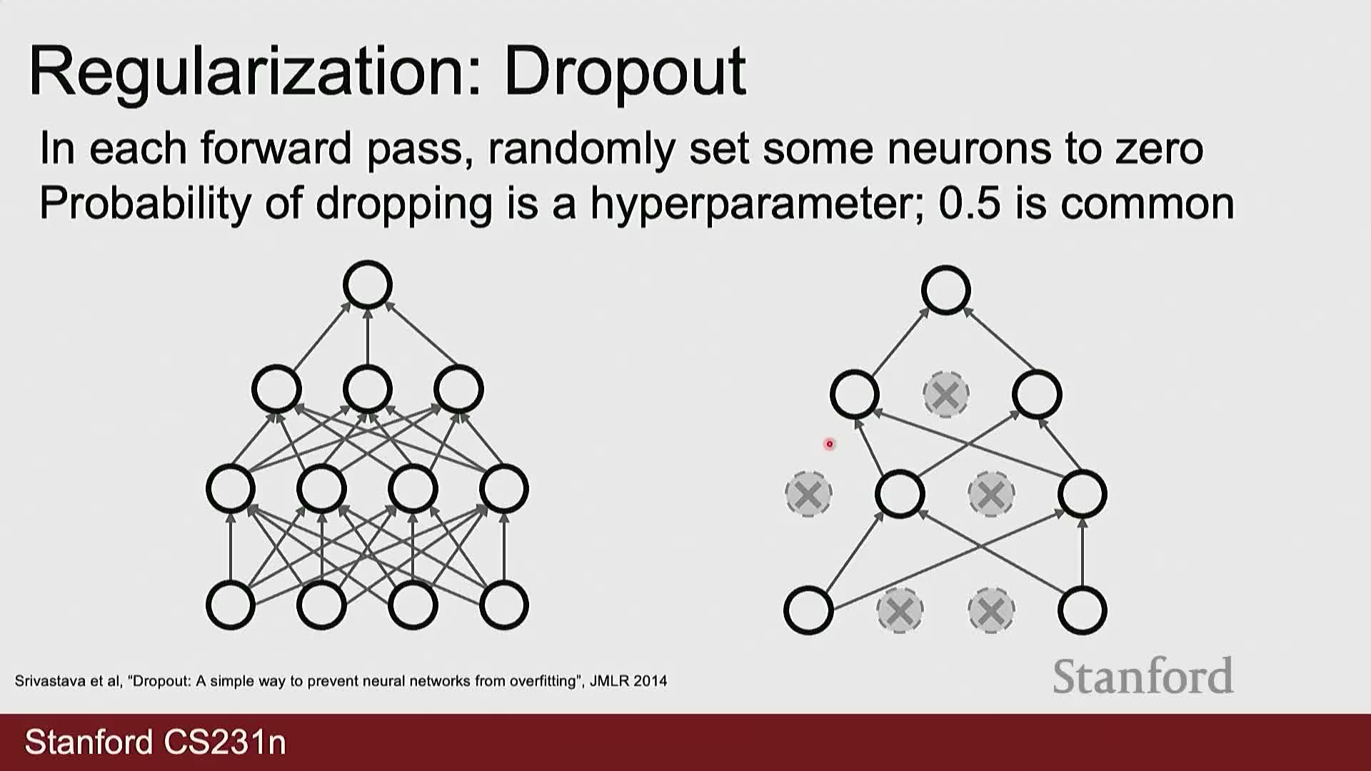
Dropout injects stochasticity during training by zeroing a fixed fraction p of activations on each forward pass.

• This forces the network to learn redundant and distributed representations and reduces co-adaptation of features.
  
• During backpropagation, gradients for dropped activations are zero, so associated weights are not updated for that pass.
  
• At test time dropout is disabled and activations are scaled by the keep probability (or equivalently training-time activations are scaled) to preserve expected activation magnitudes and avoid distribution shifts to downstream layers.
  

Nonlinear activation functions introduce expressivity; ReLU and smooth variants like GELU or CELU mitigate vanishing gradients

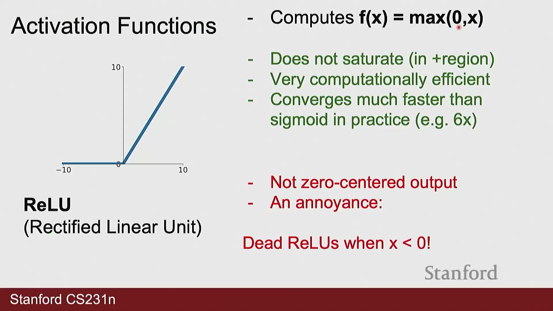
Activation functions follow linear operations (convolution or FC) to introduce the nonlinearity required for expressive modeling.

• Sigmoid: saturates for large-magnitude inputs and yields vanishing gradients, which makes deep training difficult.
  
• ReLU: avoids saturation in the positive regime (gradient = 1), is computationally cheap, but has a zero-gradient region for negative inputs (the “dead ReLU” issue).
  
• Smooth alternatives (e.g., GELU, CELU): provide nonzero gradients near zero and smoother transitions, offering numerical stability and often better empirical performance in modern architectures.
  

Classic CNN architectures stack convolutional and pooling layers then large fully connected classifiers

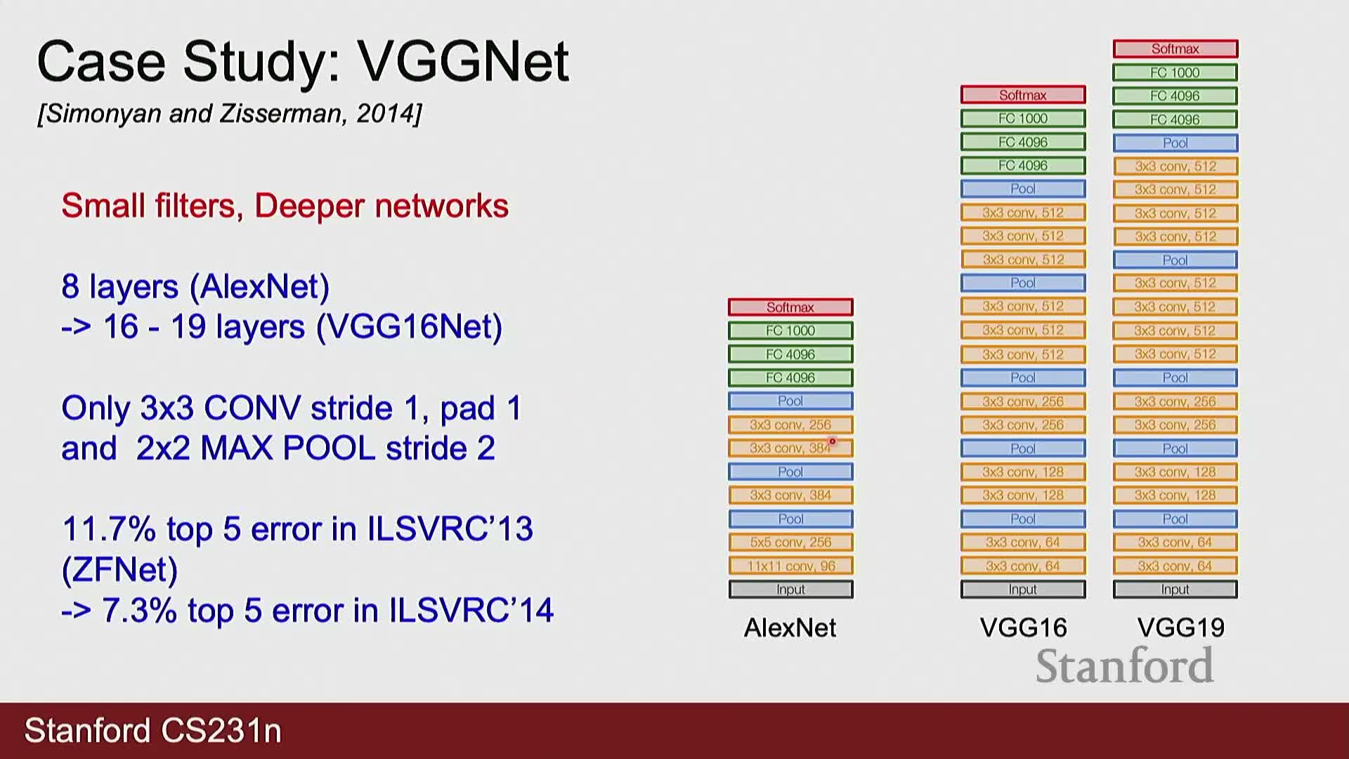
AlexNet and VGG (historic successful CNNs): composed of repeated convolutional blocks, periodic pooling, and large fully connected layers.

• VGG standardized on 3x3 filters with stride 1 and padding 1, stacking them to increase receptive field while keeping a simple, uniform design.
  
• Both use periodic max-pooling for spatial downsampling and conclude with large FC layers (e.g., two 4096-d layers in classic VGG) culminating in a final classification layer sized to the dataset’s classes.
  
• Block diagrams are useful to visualize depth, receptive field progression, and where pooling and classification occur.
  

Stacking multiple 3x3 convolutions grows the effective receptive field linearly (three 3x3 layers -> 7x7 receptive field)

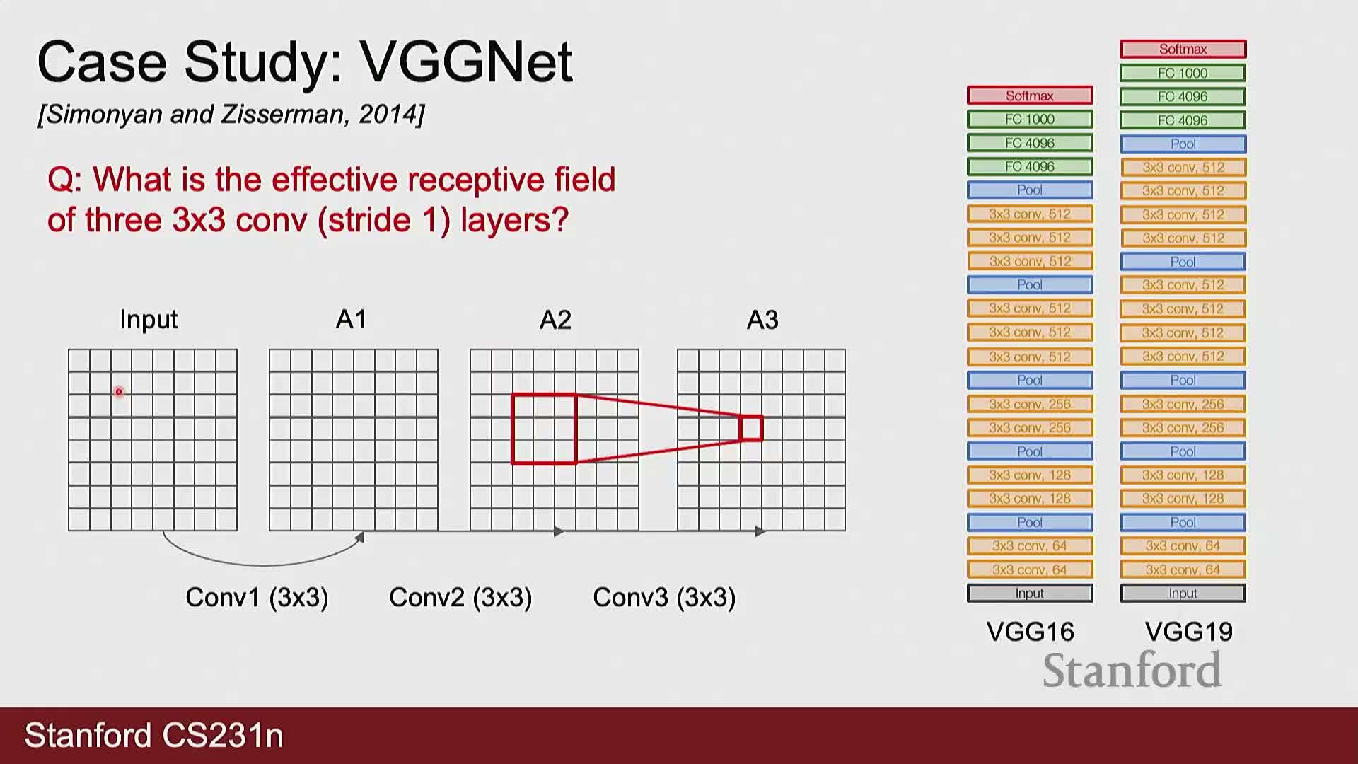
Effective receptive field quantifies the input region that influences a particular activation.

• Stacking three 3x3 convolutions with stride 1 and padding preserves spatial size while expanding the receptive field by two pixels per layer: 3x3 → 5x5 → 7x7 across three layers.
  
• This allows designers to achieve large effective receptive fields using small kernels, preserving computational and parameter advantages while introducing intermediate nonlinearities.
  

Multiple small convolutions are more parameter-efficient and more expressive than a single large convolution

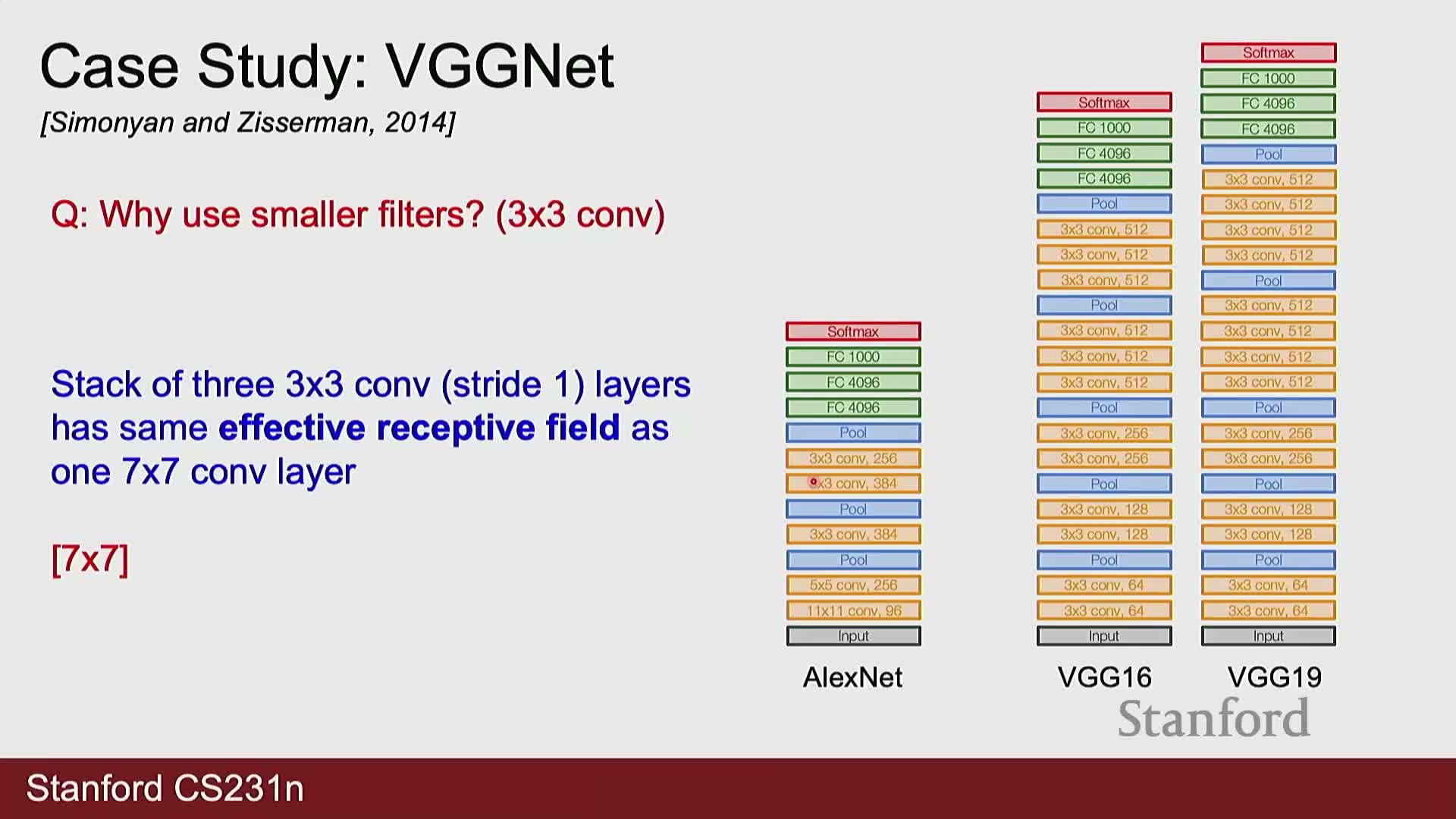
Replacing large kernels with small-kernel stacks reduces parameter count and increases representational capacity.

• Example principle: replace a single 7x7 convolution with three 3x3 convolutions.
  
• Assuming constant channel counts, the stack of three 3x3 layers typically requires fewer parameters than a single 7x7 layer and introduces additional nonlinearities between layers, enabling modeling of more complex functions with lower parameter overhead and often improved empirical performance.
  

Residual connections mitigate optimization problems in very deep networks by enabling residual learning

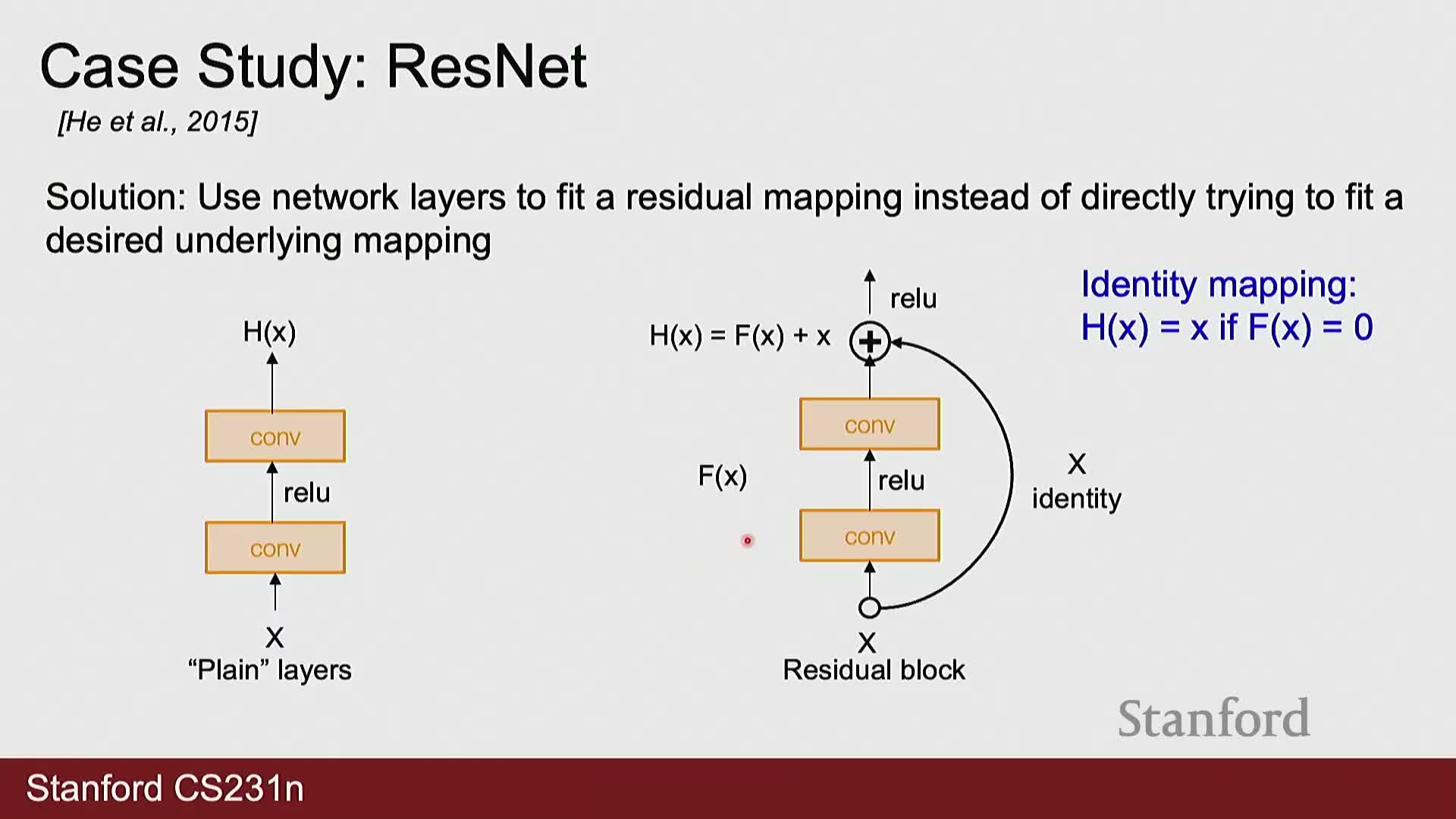
Why residual connections help optimization: deeper plain networks can be harder to optimize and may perform worse than shallower ones on training and test error.

• Residual connections redefine the mapping as a residual f(x) added to the identity x, so a block outputs x + f(x).
  
• This design makes it easy for the network to represent identity mappings (by setting f(x) ≈ 0), reducing the difficulty of optimization and enabling much deeper models to converge to lower training and test error.
  

ResNet design practices: residual blocks, stage transitions, and scalable model families

ResNet residual block and staging: a typical ResNet block and overall organization that enable deep, trainable networks.

• A ResNet block typically contains two convolutional layers with an activation between them, a skip connection that adds the input x to the block output, and a final activation.
  
• ResNets group blocks into stages, periodically downsampling spatial resolution while doubling filter counts to form deeper hierarchical features.
  
• ResNets provide a family of depths (e.g., 18, 34, 50, 101, 152) that empirically scale performance while remaining trainable due to the residual design.
  
• Minor architectural choices—such as an initial larger convolutional layer and when/how to downsample—are empirical but important for performance.
  

Kaiming (He) initialization preserves activation variance for ReLU networks by scaling by sqrt(2/fan_in)

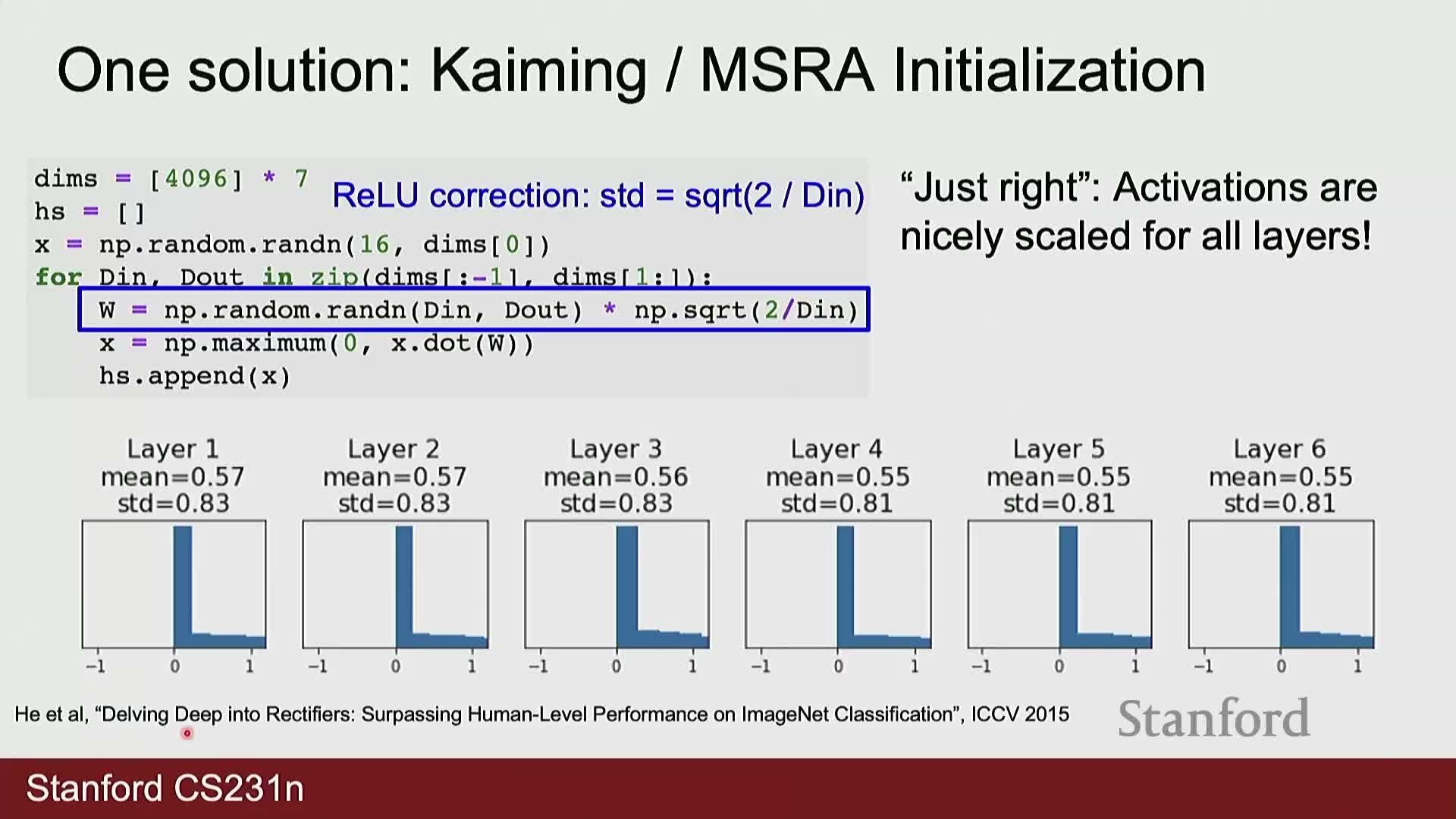
Weight initialization (Kaiming): prevents vanishing or exploding activations across many layers.

• Kaiming initialization samples weights with variance approximately 2 / fan_in (where fan_in is the number of inputs to the unit; for convolutional layers fan_in = kernel_height * kernel_width * in_channels).
  
• This choice helps keep post-activation standard deviation approximately constant for ReLU networks.
  
• Too-small initial weights drive activations toward zero across layers; too-large weights cause exponential growth. Kaiming is the standard practical choice for ReLU-based CNNs.
  

Image preprocessing standardizes RGB channels by dataset mean and standard deviation

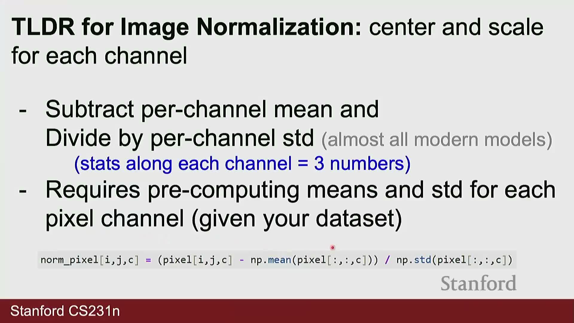
Image preprocessing: normalize pixel-level statistics to reduce covariate shift.

• Common practice: compute per-channel mean and standard deviation over the dataset (or use established statistics such as ImageNet means/stds).
  
• Normalize each input image by subtracting the channel mean and dividing by the channel standard deviation.
  
• Benefits: reduces pixel-level covariate shift, accelerates convergence, and produces consistent inputs when reusing pretrained weights.
  

Data augmentation increases training diversity and improves generalization by applying label-preserving transformations at train time

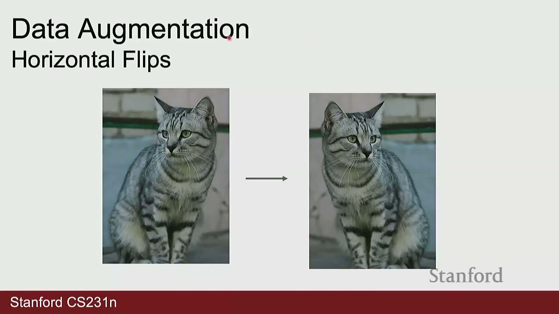
Data augmentation: apply randomized transformations to training examples to simulate extra data and reduce overfitting.

• Typical transforms include flips, crops, color perturbations, noise, and occlusions.
  
• Canonical pattern: apply stochastic perturbations at training time. Optionally, average model predictions over multiple deterministic augmentations at test time (test-time augmentation) for marginal accuracy gains.
  
• Augmentation increases effective dataset size, often raises training loss (making training harder) but improves validation performance by regularizing the model.
  

Common image augmentations include horizontal flip, random resized crop, multi-crop test-time augmentation, color jitter, and cutout

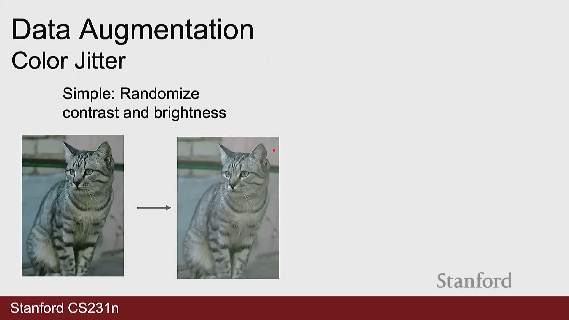
Common augmentation techniques and practical tips: choose augmentations that preserve label semantics.

• Horizontal flipping: appropriate when left-right symmetry does not change labels; vertical flips or rotations depend on the domain.
  
• Random resized crop: preserve aspect ratio by resizing the short side to a chosen scale L, then sample a random 224x224 crop for models using 224 input—this yields translation and scale robustness.
  
• Test-time augmentation: average predictions across multiple crops/scales/flips to gain ~1–2% accuracy in many settings.
  
• Color jitter (brightness/contrast/saturation) and occlusion techniques (cutout) simulate sensor and occlusion variability; tune strengths so augmented images remain recognizably in-distribution to humans.
  

Transfer learning strategies: freeze pretrained features for very small datasets or fine-tune entire networks for larger similar datasets

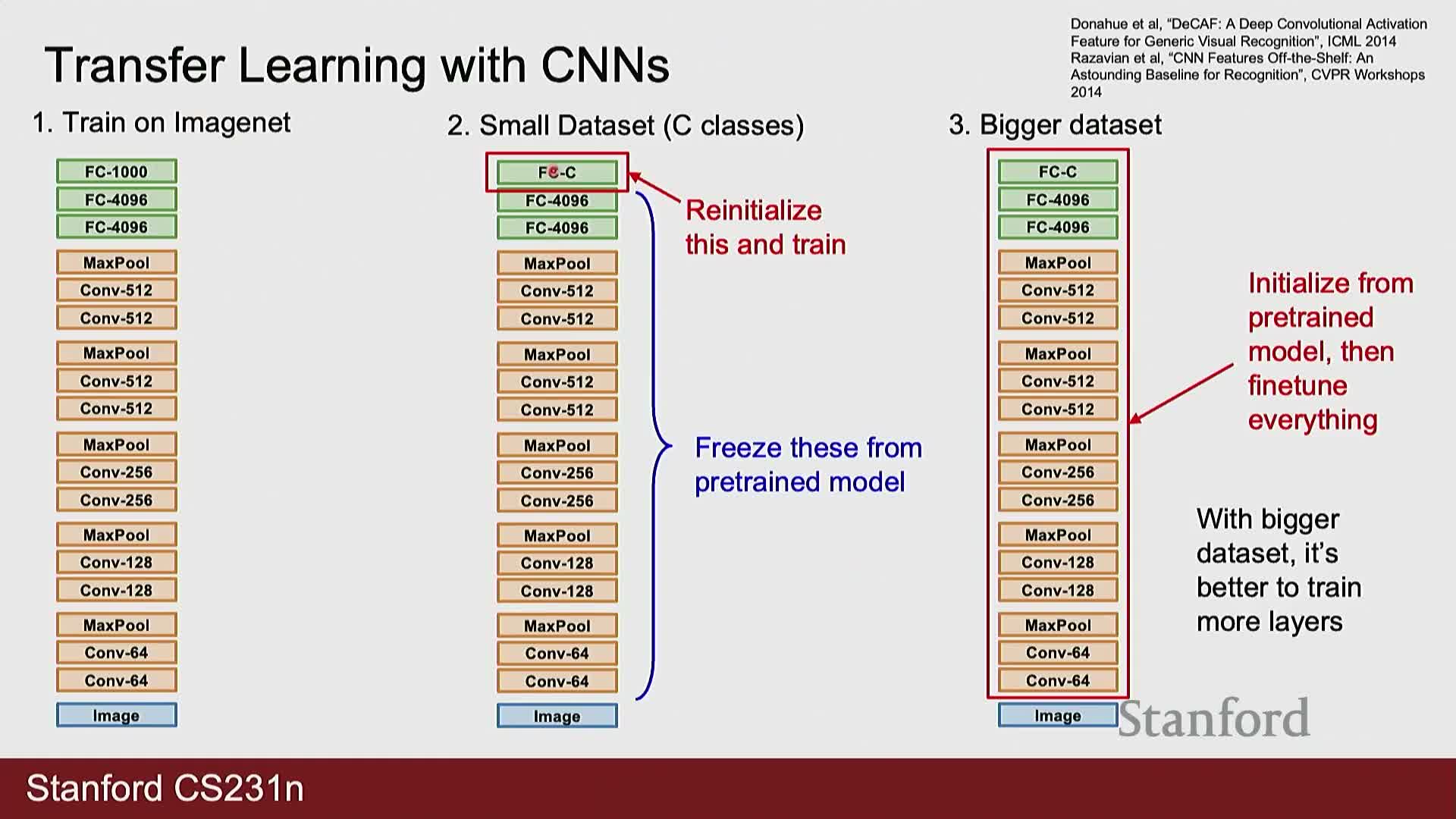
Transfer learning strategies for limited data: leverage pretrained models when target data is scarce and similar to a large pretraining corpus (e.g., ImageNet).

1. Frozen feature extractor: use a pretrained network as a fixed feature extractor and train only a new final classifier—avoids overfitting small datasets.
   
2. Fine-tuning: initialize from pretrained weights and fine-tune all (or many) layers when sufficient labeled data exists—adapts representations to the target domain.
   

• For out-of-distribution target domains, pretrained initialization may still help but introduces bias; consider domain-specific methods (including low-rank adaptation techniques) when appropriate.
  

Hyperparameter debugging and search: overfit a tiny dataset to validate implementation, then use coarse random search for tuning

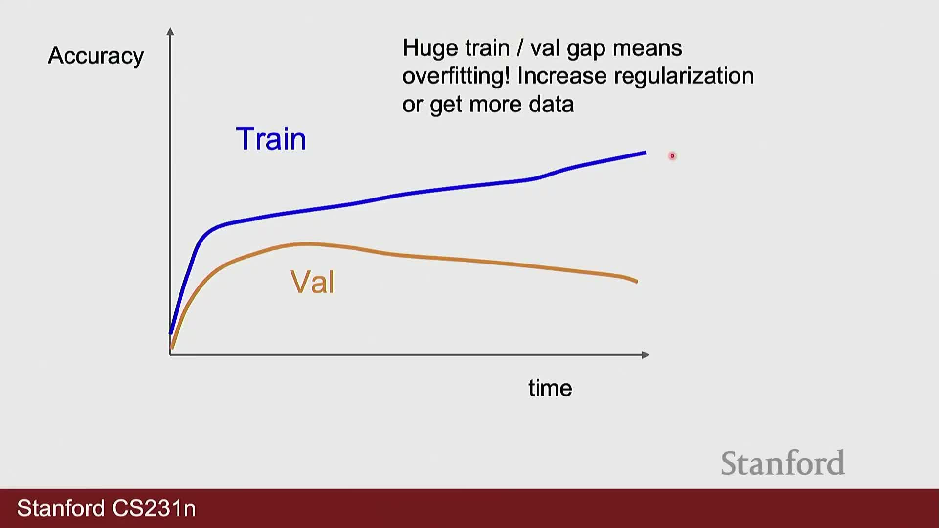
Debugging and hyperparameter selection (practical steps): systematic checks and tuning procedures.

1. Overfit a tiny subset: confirm the implementation and optimizer can drive training loss near zero on a very small dataset—this exposes bugs or inappropriate settings.
   
2. Learning-rate discovery: run coarse experiments to find viable learning-rate regimes before fine-grained tuning.
   
3. Randomized hyperparameter search: perform randomized searches across defined parameter ranges rather than exhaustive grid search to efficiently explore promising regions.
   
4. Monitor metrics: track training and validation losses and accuracies for signs of underfitting, overfitting, or divergence; adjust regularization, augmentation, or learning-rate schedules accordingly.