Stanford CS231N | Spring 2025 | Lecture 7- Recurrent Neural Networks
- Clarification of dropout scaling at test time
- Normalization reduces but does not eliminate sensitivity to poor weight initialization
- Practical tooling for hyperparameter exploration improves model tuning
- Sequence modeling generalizes fixed-size input/output networks to variable-length data
- Sequence tasks are categorized as one-to-many, many-to-one, or many-to-many
- An RNN maintains and updates a hidden state across time steps
- RNN forward equations use shared parameterized functions for state update and output mapping
- Designing a hidden state requires encoding the minimal sufficient information for the task
- Manual construction of recurrent weight matrices demonstrates how inputs, state copying, and outputs are implemented
- Weight matrices in RNNs are learned by gradient descent across time steps
- Backpropagation through time (BPTT) computes gradients across the unrolled recurrence and can be memory intensive
- Chunking and truncated BPTT trade off exact gradient flow for tractability
- Character-level RNN language models perform timestep classification and use embeddings for inputs
- Hidden activations in RNNs can be highly interpretable and reveal task-specific detectors
- RNNs offer unlimited context length and parameter efficiency but suffer from sequential computation and limited capacity
- RNN-based architectures were widely used for vision-language tasks like captioning, VQA, and visual navigation
- Multi-layer RNNs stack recurrent layers vertically while sharing weights across time within each layer
- Vanishing and exploding gradients arise from repeated multiplication by activation derivatives and recurrent weight matrices
- LSTMs introduce gating and a separate cell pathway to improve long-term information flow
- Skip connections and highway pathways parallel ResNet ideas and enable long-range signal propagation
- Recent work revives recurrent and state-space approaches to address transformer context and scaling limits
Clarification of dropout scaling at test time
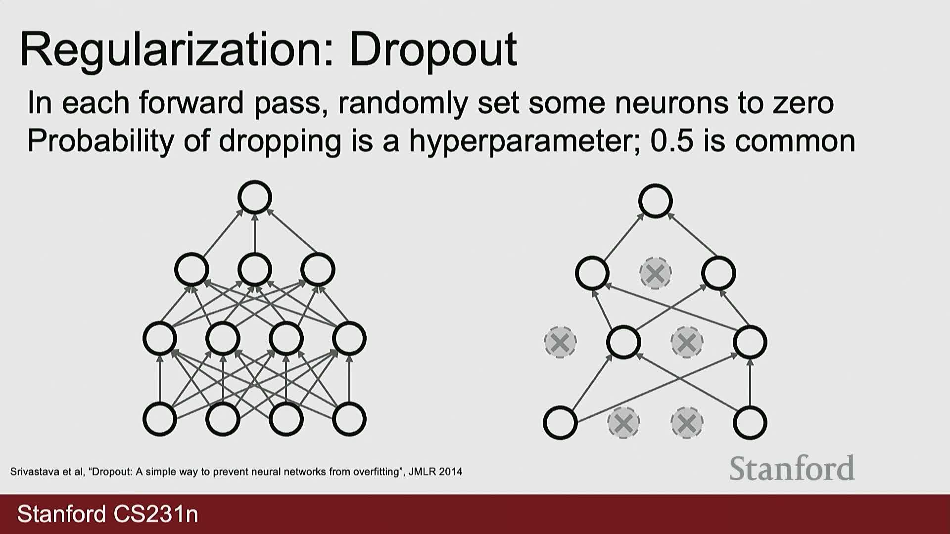
Dropout at training time randomly zeroes activations using a Bernoulli mask parameterized by P—which may be interpreted either as the drop probability or the keep probability depending on the implementation.
- At test time the network must scale activations so the expected activation magnitude matches training to avoid distributional mismatch and downstream bias.
- The common convention in many libraries treats P as the drop probability and therefore scales activations at test time by (1 - P) when the implementation drops units during training.
- Implementations that treat P as the keep probability do not perform test-time scaling because the forward pass already preserves expectation in that formulation.
Carefully handling this distinction when reading or porting code across frameworks is essential to avoid mismatches between training and inference behavior.
Normalization reduces but does not eliminate sensitivity to poor weight initialization
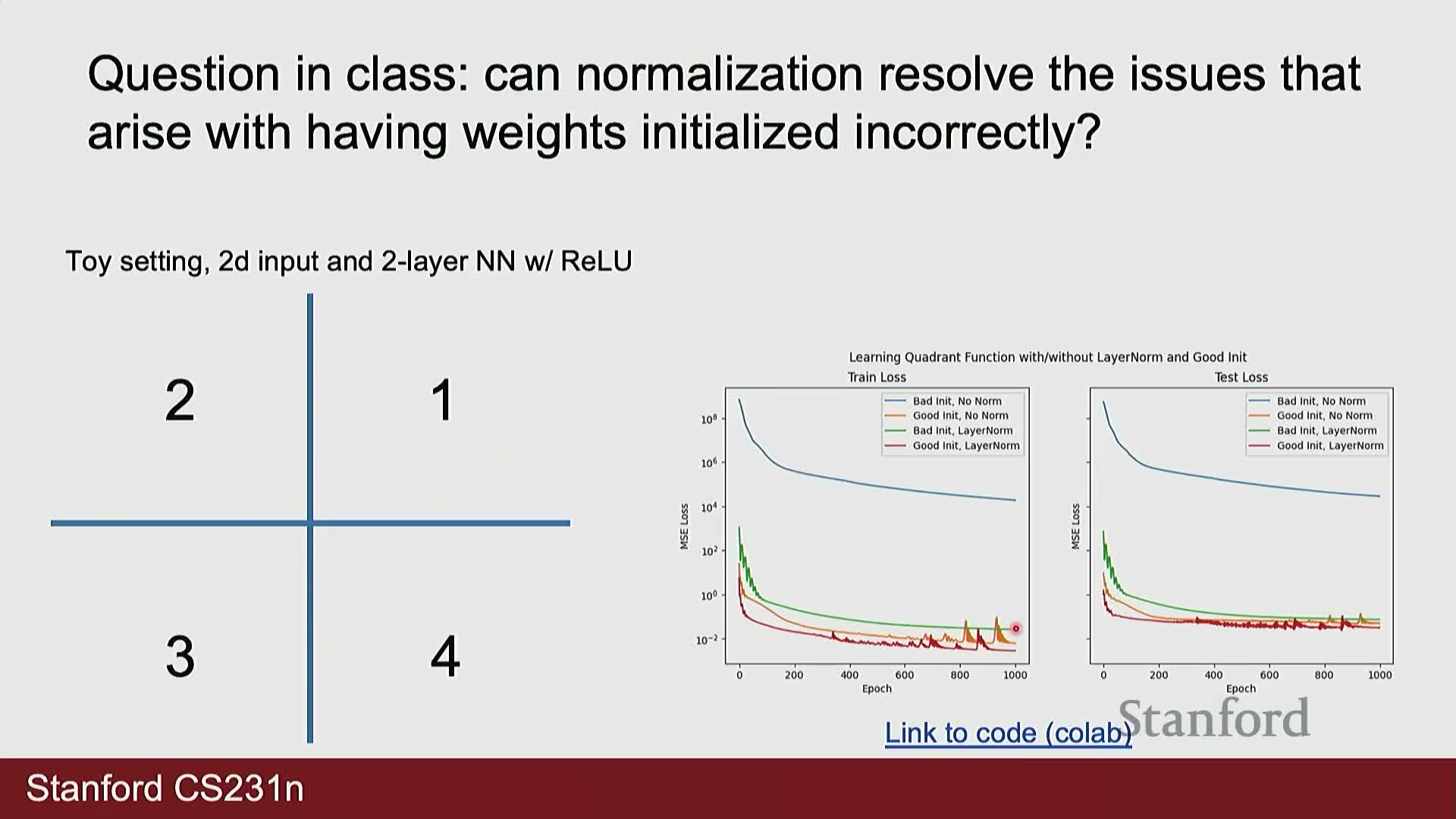
Normalization techniques such as layer normalization or batch normalization can mitigate training instabilities caused by poor weight initialization by centering and scaling activations, which improves gradient flow and optimization dynamics.
- Empirically, normalization often narrows the gap between good and bad initializations but does not replace sensible initialization schemes (for example Kaiming/He initialization) for optimal performance.
- Normalization can also harm tasks that require preservation of absolute spatial or value information, because subtracting a mean and dividing by a standard deviation can remove signal needed for precise outputs.
In short: normalization is a valuable optimization tool but not a universal remedy—their benefit depends on the task and data representation.
Practical tooling for hyperparameter exploration improves model tuning
Systematic experiment tracking platforms enable comparative analysis of hyperparameters and validation metrics across many runs, making selection and debugging of learning rate schedules, regularization, and architecture variants easier.
- Visualizations that encode hyperparameters (for example via color or columns) help reveal trends, such as how varying dropout correlates with validation accuracy.
- These tools complement techniques like test-time augmentation and transfer learning by simplifying management and interpretation of many experiments, especially when compute allows repeated trials.
- Common options include both open-source tools and hosted services; the choice is a workflow preference, but consistent logging and visualization is essential for reproducible model development.
Sequence modeling generalizes fixed-size input/output networks to variable-length data
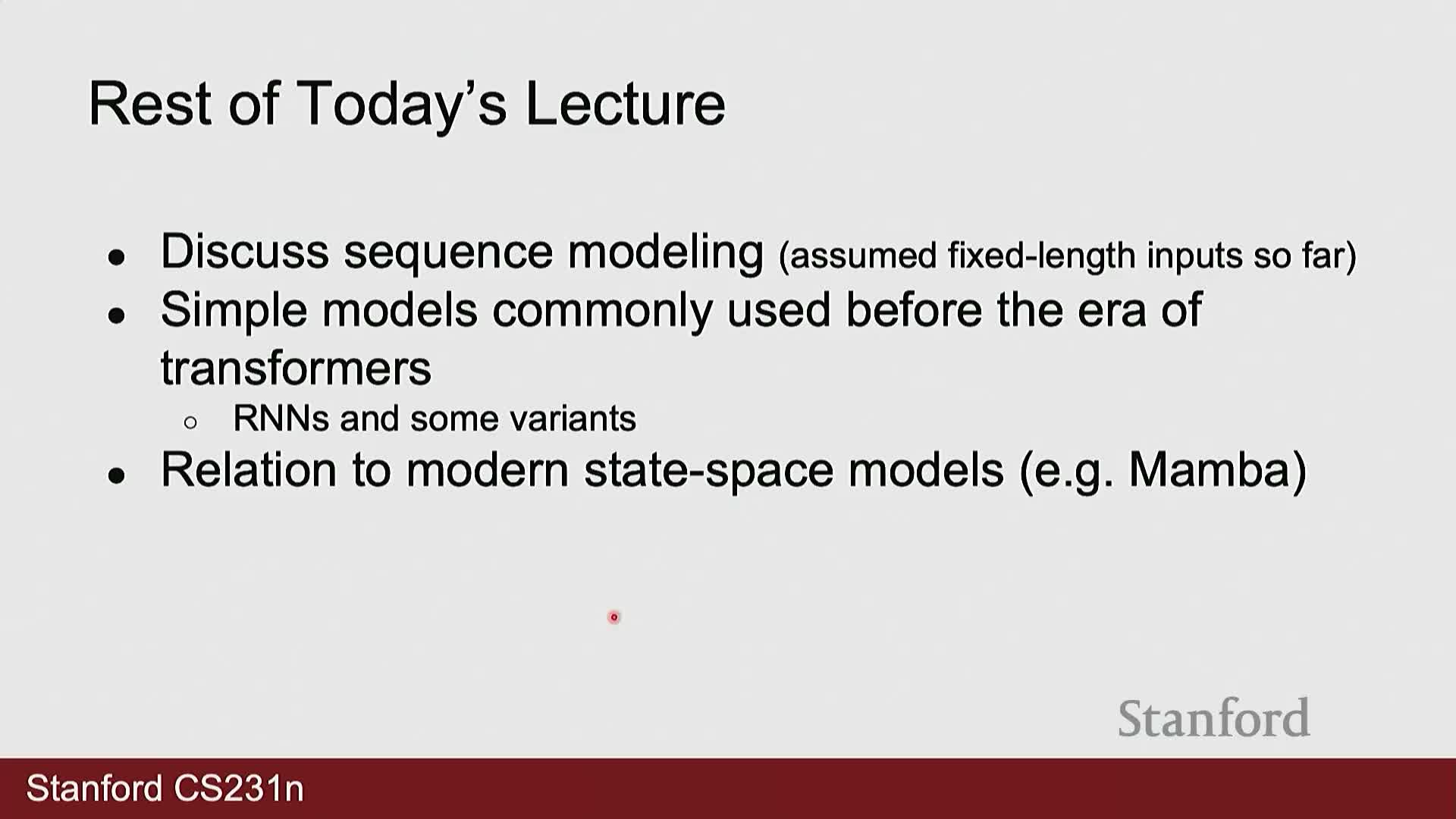
Sequence modeling addresses problems where input and/or output lengths vary across examples, in contrast to fixed-size input-output setups used for images or tabular data.
- Typical formulations:
- One-to-many (e.g., image → caption)
- Many-to-one (e.g., video sequence → single class)
-
Many-to-many (e.g., per-frame video labeling or token-by-token language tasks)
- Modeling choices:
- May require coupling of modalities (for example a CNN encoder plus a sequence decoder)
- May require autoregressive feeding of prior outputs into future inputs
Understanding these paradigms clarifies which architectural motifs (encoder, decoder, autoregression) and training strategies (per-step loss vs. terminal loss) are appropriate for a given problem.
Sequence tasks are categorized as one-to-many, many-to-one, or many-to-many
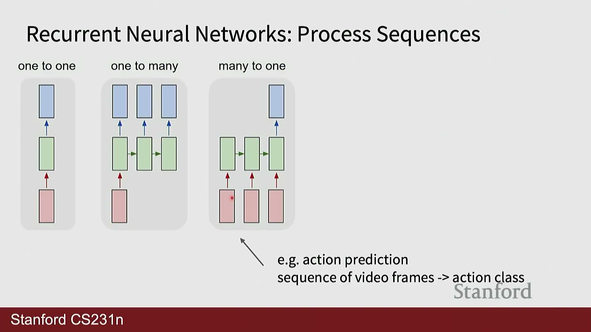
One-to-many, many-to-one, and many-to-many categorizations guide architecture and training decisions for sequence tasks.
- Architecture implications:
- An encoder–decoder structure is often required for input→variable-length output problems.
-
Recurrence, attention, pooling, or sequence-to-sequence mechanisms are chosen based on the mapping type.
- Loss placement and training:
- Decide between per time-step losses (supervise each output) or a terminal loss (supervise only the final output).
- Training/inference techniques include teacher forcing or autoregressive sampling to handle sequential generation.
- Practical systems often mix paradigms (e.g., apply pooling over time to convert many-to-many into many-to-one), so mapping an application onto one formulation guides necessary small adaptations.
An RNN maintains and updates a hidden state across time steps
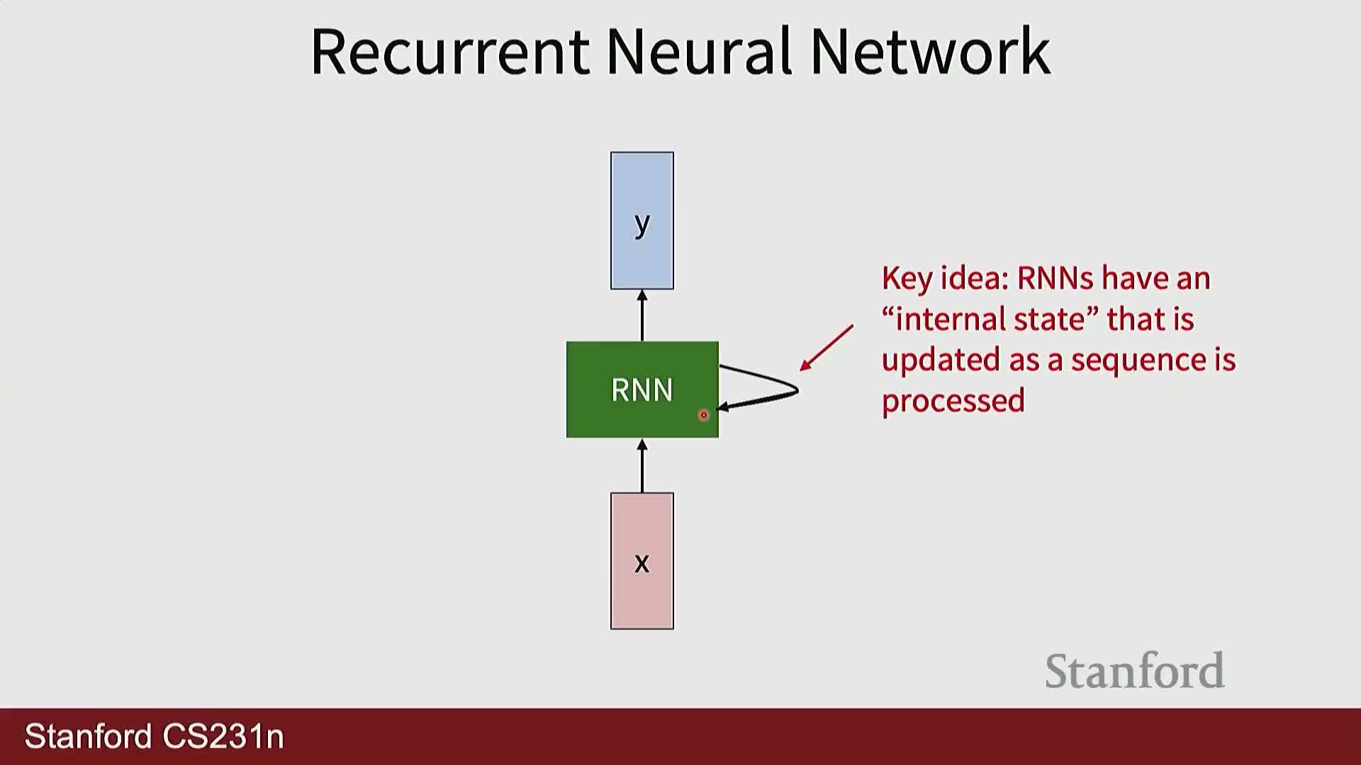
A recurrent neural network (RNN) is defined by a hidden (internal) state that is updated each time step via a fixed recurrence: the new hidden state is a function of the previous hidden state and the current input.
- Typical structure:
- The recurrence is parameterized by shared weight matrices and a nonlinear activation.
- An output function (with separate weights) optionally computes per-step or terminal predictions from the hidden state.
- Unrolling the recurrence across time:
- Clarifies forward computation order.
- Enables backpropagation through time (BPTT) by converting the loop into an explicit computational graph.
-
Weight sharing across time steps provides parameter efficiency and enforces the same computation at every time point, reflecting a stationarity assumption in many sequence tasks.
RNN forward equations use shared parameterized functions for state update and output mapping
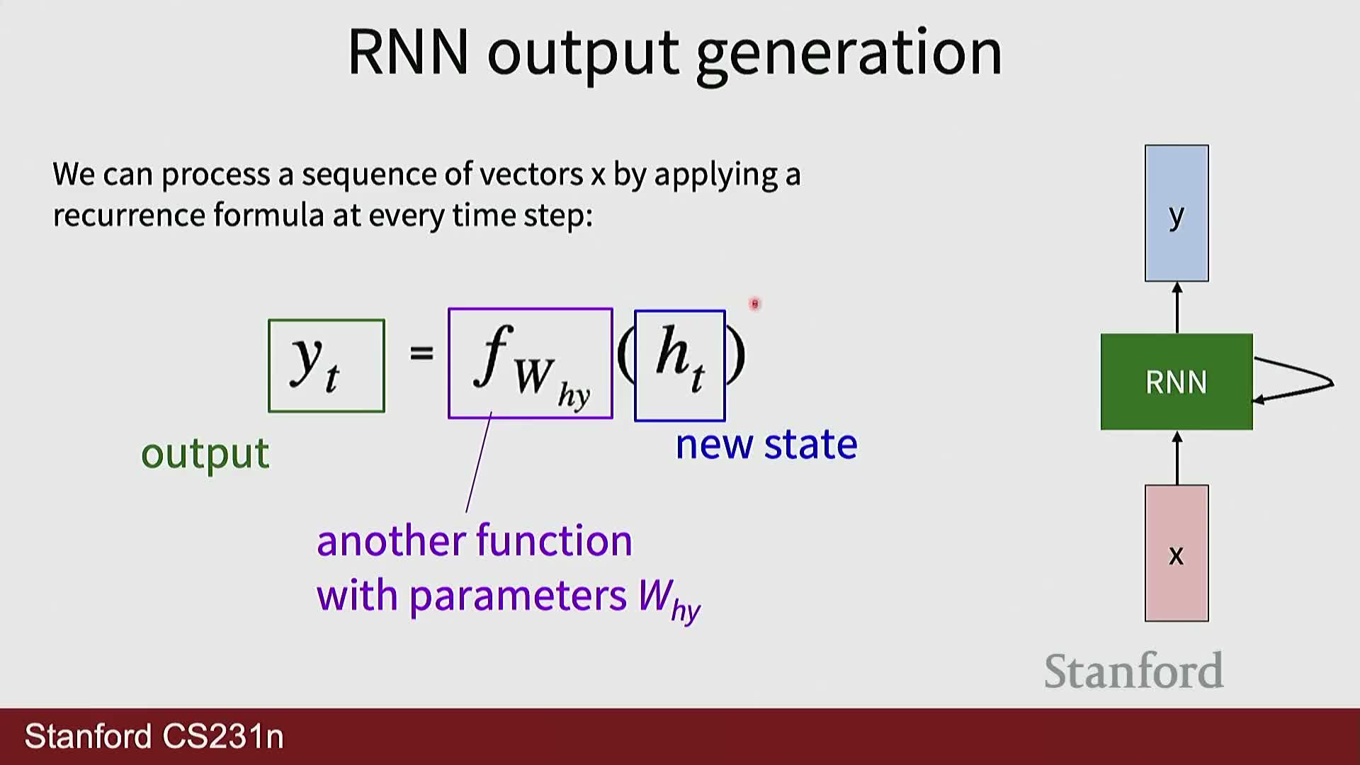
Formally, a recurrence computes h_t = f(h_{t-1}, x_t; W) where f is usually an affine transform followed by a nonlinear activation, and the output y_t = g(h_t; V) maps hidden states into output space.
- Roles and properties:
- W (shared across time) applies the same transform to each sequence element while the hidden state carries context.
- Activation choice (for example tanh or ReLU) controls dynamic range and gradient behavior.
- Output mappings can include linear layers and softmax for classification tasks.
- Training implications:
- Gradients accumulate from all time steps with respect to the same recurrent weights.
- Distinguishing the update weights (W) from the output mapping (V) clarifies that output layers may have different dimensionalities or losses depending on the task.
Designing a hidden state requires encoding the minimal sufficient information for the task
When constructing an RNN—by design or learning—the hidden state must compactly capture information needed for future outputs (for example, current and previous inputs when detecting repeats).
- Pedagogical toy example:
- Use a three-dimensional hidden vector encoding: current input, immediately previous input, and a constant bias, to illustrate how matrix multiplications implement state-shifting and feature extraction.
- Use a three-dimensional hidden vector encoding: current input, immediately previous input, and a constant bias, to illustrate how matrix multiplications implement state-shifting and feature extraction.
- Practical notes:
- The initial hidden state H0 can be learned or initialized to a default and can significantly affect early-step outputs.
- Design choices influence interpretability and the complexity required to represent temporal dependencies.
This thought experiment makes explicit how weight matrices implement memory update, copy, and selection operations in the recurrent pathway.
Manual construction of recurrent weight matrices demonstrates how inputs, state copying, and outputs are implemented
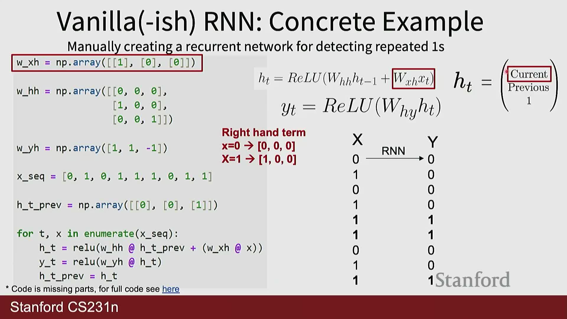
Concrete RNN implementations typically use two primary matrices: an input-to-hidden matrix and a hidden-to-hidden matrix.
- Roles:
- The input-to-hidden matrix maps the current input into hidden dimensions.
- The hidden-to-hidden matrix transforms and copies components of the previous hidden state into positions representing “previous” values.
- Activation and readout:
- Using ReLU with binary inputs simplifies behavior to max(0,·) operations so carefully chosen weights can produce exact logical behaviors (for example copying a 1 into a previous slot).
- The output weight vector then linearly combines hidden components (e.g., current + previous − bias) to produce desired outputs after activation.
This construction clarifies how matrix structure realizes memory shift, gating, and readout in recurrent architectures and parallels learned parameters in general RNNs.
Weight matrices in RNNs are learned by gradient descent across time steps
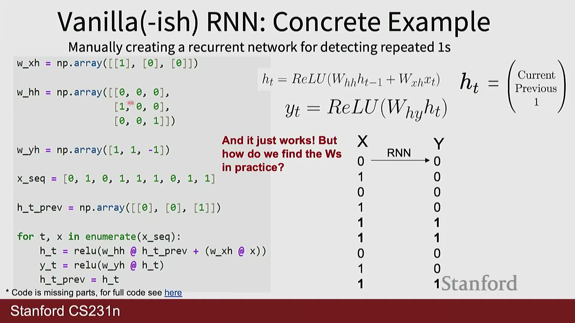
Although toy RNNs can be hand-crafted, practical RNNs obtain weight matrices via gradient-based optimization, summing contributions from losses across time steps where the same recurrent matrix is reused.
- Optimization view:
- The optimizer accumulates per-time-step gradients for shared parameters (conceptually treating the recurrent application as many tied layers) and then applies updates using the chosen optimizer and learning rate.
- The optimizer accumulates per-time-step gradients for shared parameters (conceptually treating the recurrent application as many tied layers) and then applies updates using the chosen optimizer and learning rate.
- Computational considerations:
- Training across many time steps requires storing activations for the unrolled steps to compute gradients unless truncation or checkpointing is applied.
- Recognizing that the same parameter set is optimized across time clarifies both the efficiency of parameter reuse and the source of temporal credit assignment in sequence learning.
Backpropagation through time (BPTT) computes gradients across the unrolled recurrence and can be memory intensive
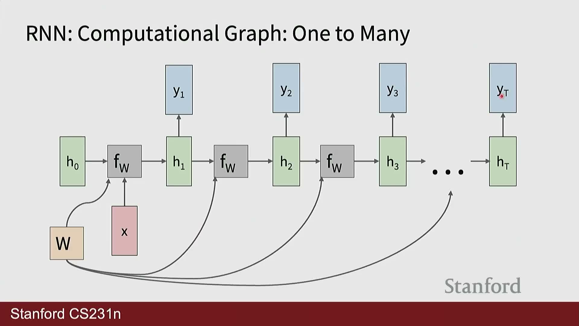
Backpropagation through time (BPTT) treats the unrolled RNN as a deep feedforward graph across time and computes gradients by applying the chain rule backward through each time step, summing parameter gradients accumulated at each step.
- Practical costs and issues:
- Long sequences require storing activations and intermediates for many timesteps, resulting in high memory usage and potential numerical instability (for example NaNs) if gradients explode.
- Long sequences require storing activations and intermediates for many timesteps, resulting in high memory usage and potential numerical instability (for example NaNs) if gradients explode.
- Practical remedy — truncated BPTT:
- Limit gradient computation to a sliding fixed-size time window.
- Propagate gradients only over that window while passing the final hidden state as the initial state for the next window.
Truncation reduces memory and compute at the expense of exact long-range gradient propagation and is widely used for long-sequence training.
Chunking and truncated BPTT trade off exact gradient flow for tractability
Truncated BPTT partitions a long sequence into chunks, computes forward and backward passes within each chunk, and transfers the final hidden state to the next chunk while discarding per-step activations to save memory.
- Mechanics:
- Each chunk does a forward pass and computes gradients only within that chunk.
- The final hidden state (and optionally a compact gradient summary) is passed forward; per-step activations are discarded to conserve memory.
- Consequences and analogy:
- Training yields multiple gradient estimation steps over disjoint windows whose summed updates approximate full BPTT.
- This mirrors distributed gradient computation where independent workers compute partial gradients and those gradients are aggregated.
- Caveat:
- Information and gradient signals beyond the truncation window are approximated rather than exact, which can hinder learning very long-range dependencies.
- Information and gradient signals beyond the truncation window are approximated rather than exact, which can hinder learning very long-range dependencies.
Character-level RNN language models perform timestep classification and use embeddings for inputs
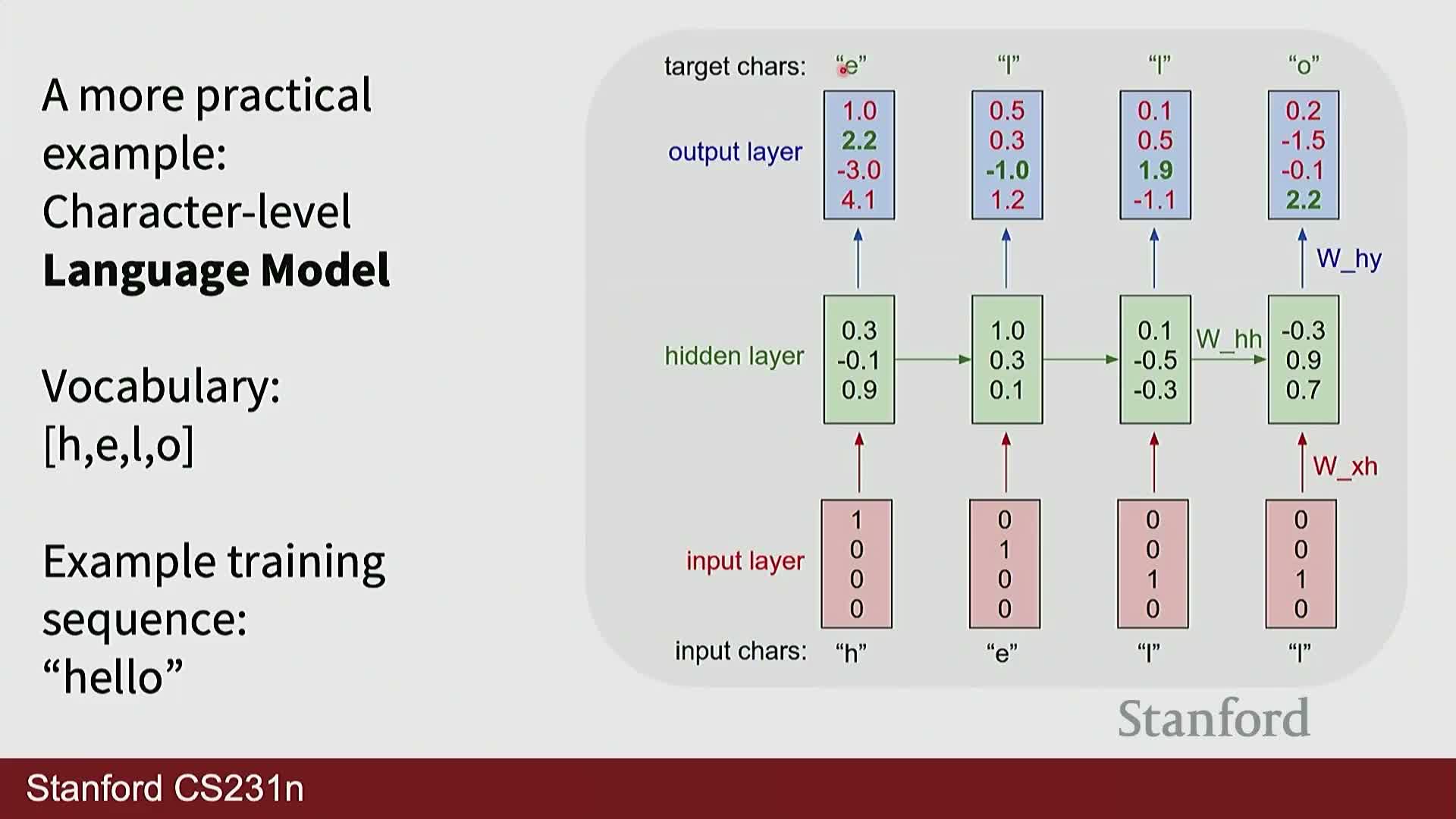
Character-level language models treat sequence prediction as a per-time-step classification over the next token.
- Input and embeddings:
- Each input token is commonly encoded as a one-hot index and mapped through a learned embedding matrix into a dense vector before the recurrent layer.
- The embedding matrix (one vector per token) is trained jointly and replaces sparse one-hot representations with dense features that aid optimization and generalization.
- Decoding and inference:
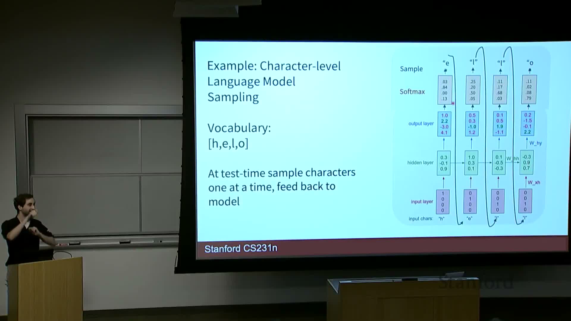
- At inference the model decodes autoregressively by feeding generated tokens back as inputs to produce subsequent tokens.
- Decoding strategies include greedy selection, sampling, or beam search to balance diversity and likelihood.
These models learn rich structure from raw sequential corpora because next-token supervision is inherent in the data.
Hidden activations in RNNs can be highly interpretable and reveal task-specific detectors
Examining individual hidden units or channels across time often exposes interpretable signals such as quote detectors, line-length predictors, indentation counters, or comment/if-statement detectors.
- Analysis techniques:
-
Activation heatmaps across characters or tokens show when particular units turn on or off and how the network represents stateful properties like nesting depth.
-
Activation heatmaps across characters or tokens show when particular units turn on or off and how the network represents stateful properties like nesting depth.
- Implications:
- Interpretable neurons indicate recurrent layers can learn specialized memory-like computations without explicit supervision for those features.
- Such analyses can guide debugging, pruning, or architectural choices, and explain why RNNs were historically effective for sequence modeling.
RNNs offer unlimited context length and parameter efficiency but suffer from sequential computation and limited capacity
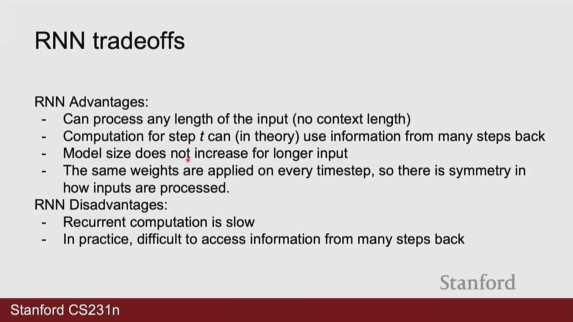
RNNs process sequences inherently sequentially: each step depends on the prior hidden state, which gives them theoretical access to arbitrarily long context without increasing parameter count.
- Trade-offs:
- Parameter efficiency: RNNs reuse the same parameters across time, unlike architectures that allocate per-position parameters.
- Parallelism cost: The sequential dependency hampers parallelism and batching during training because timesteps cannot be trivially computed independently.
-
Capacity limit: The fixed-size hidden state must compress potentially vast history, making long-range dependency retention difficult and causing information loss as context grows.
These trade-offs explain why RNNs remain attractive for very long-context problems but face scaling and optimization challenges that motivated alternative architectures.
RNN-based architectures were widely used for vision-language tasks like captioning, VQA, and visual navigation
Historically, CNN encoders combined with RNN decoders formed the backbone of image captioning systems: a pre-trained CNN produced a fixed visual representation that initializes or conditions an RNN, which decodes a word sequence autoregressively until an end token is sampled.
- Variants and tasks:
- Visual question answering (VQA) can be framed as generative sequence modeling over text answers or as discriminative classification over candidate answers; both have used recurrent decoders or sequence encoders.
-
Visual navigation and visual dialogue tasks used recurrent state tracking to output sequential decisions or turn-based language, with the RNN hidden state serving as memory of observed visual context and prior dialog turns.
- Limitations:
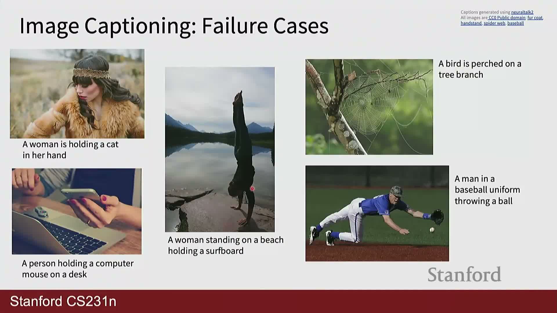
- These CNN+RNN pipelines achieved strong empirical results but were subject to dataset bias and hallucination tied to co-occurrence statistics and the modeling objective.
- These CNN+RNN pipelines achieved strong empirical results but were subject to dataset bias and hallucination tied to co-occurrence statistics and the modeling objective.
Multi-layer RNNs stack recurrent layers vertically while sharing weights across time within each layer
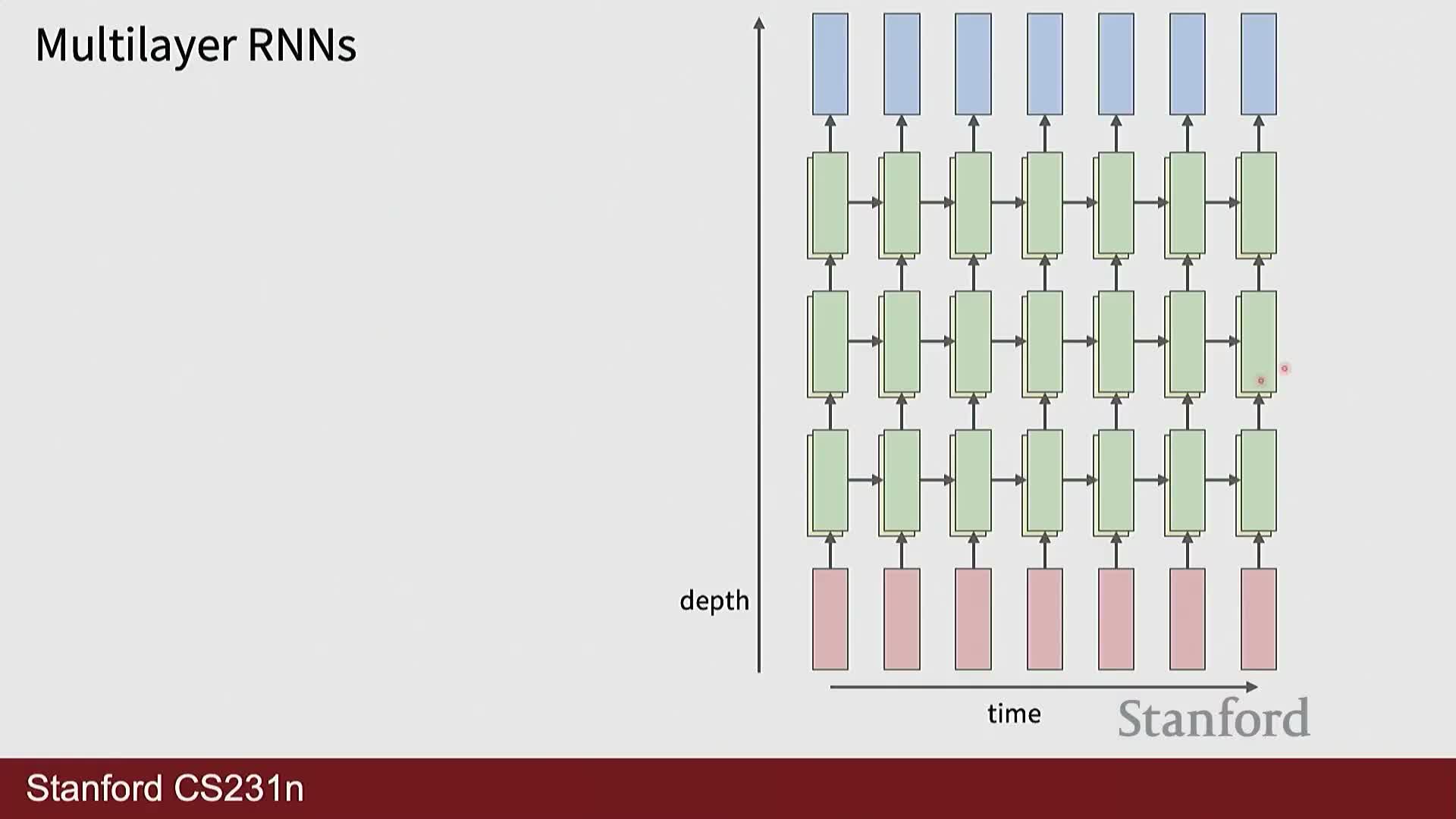
Deep RNN architectures add recurrence along both time and depth: each recurrent layer maintains its own hidden state across time and applies its own weights, while higher layers receive the lower layer’s hidden state at the same time step.
- Structure:
- Recurrence within each layer depends on that layer’s previous hidden state; vertical connections propagate information between layers at the same time index.
- The resulting grid-like computational graph increases representational capacity.
- Costs and trade-offs:
- More nodes must be computed and stored for backpropagation, amplifying memory and computation demands compared to single-layer RNNs.
- Choosing layer counts and widths trades off modeling power against training complexity and resource constraints.
Vanishing and exploding gradients arise from repeated multiplication by activation derivatives and recurrent weight matrices
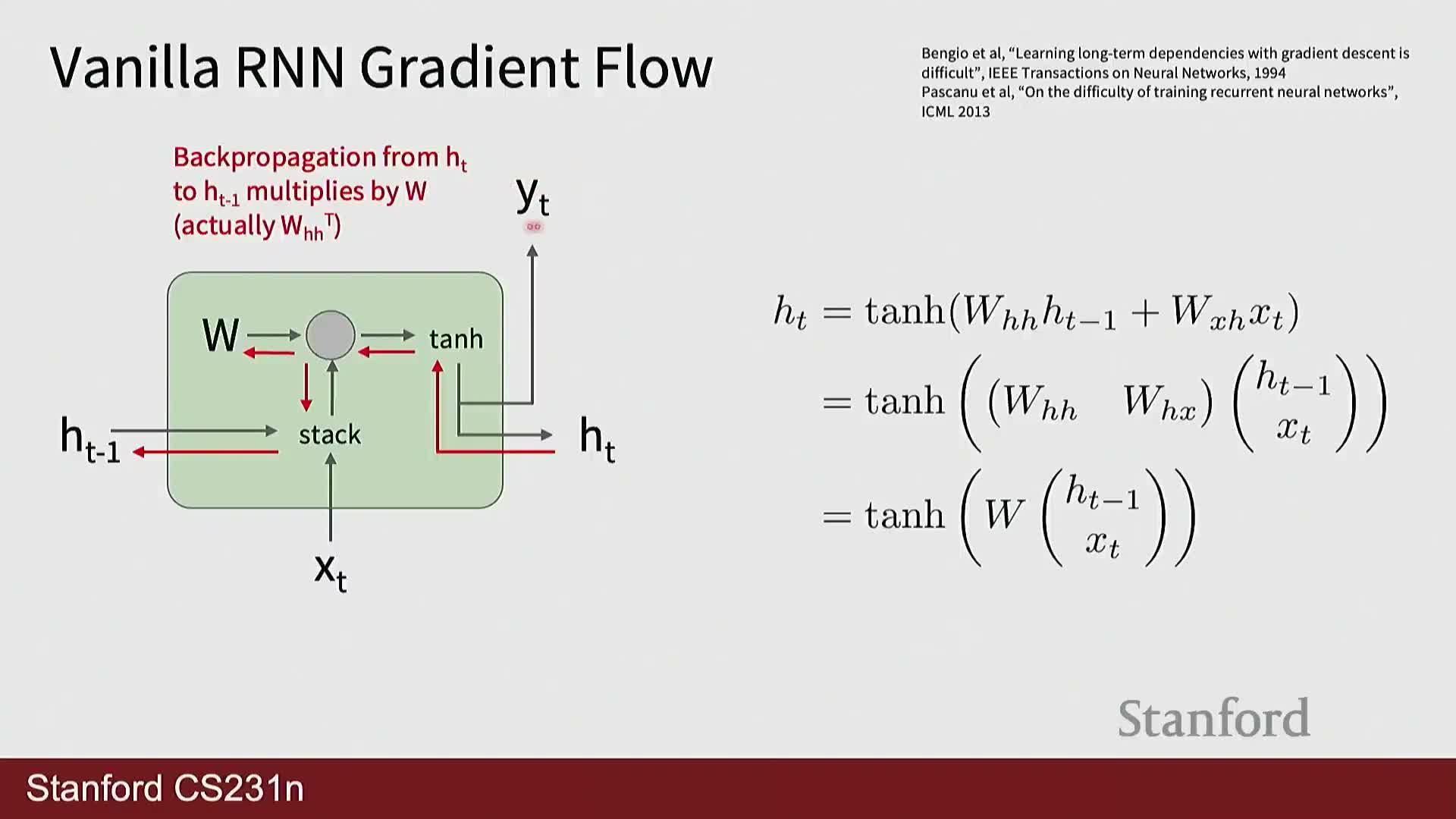
Backpropagating gradients through many time steps repeatedly applies activation derivatives (for example the derivative of tanh, bounded by 1) and multiplies by the recurrent weight matrix—this can cause gradients to vanish or explode depending on spectral properties and activation behavior.
- Mathematical intuition:
- The product of Jacobians across steps determines gradient magnitude.
- If the largest singular value of the recurrent matrix is < 1 and activation derivatives are small, gradients tend to vanish.
- Very large singular values or unstable parameter regimes produce exploding gradients.
- Mitigations:
- Exploding gradients can be mitigated by techniques such as gradient clipping.
-
Vanishing gradients are harder to address because small gradients impede learning of long-term dependencies—this motivates architectural changes and specialized recurrence schemes.
LSTMs introduce gating and a separate cell pathway to improve long-term information flow
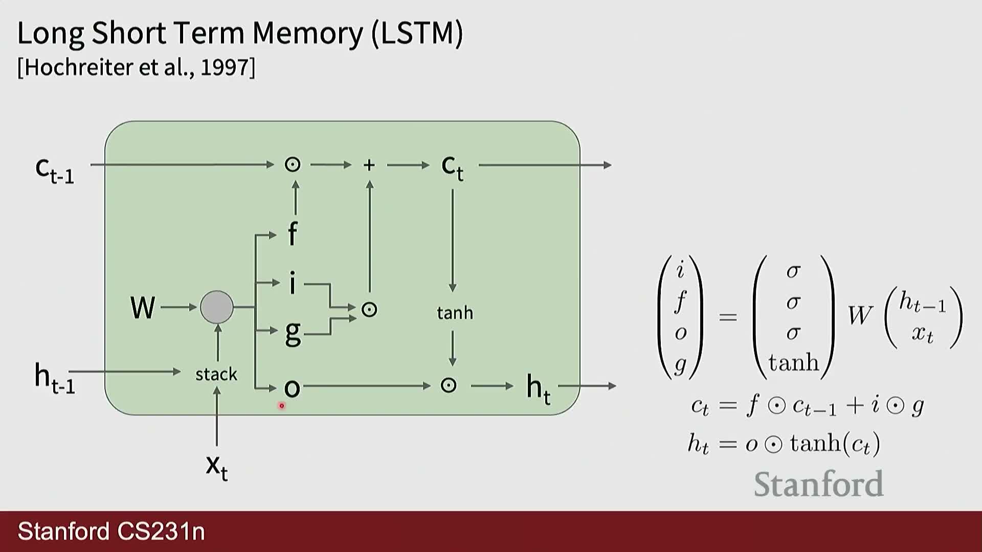
Long Short-Term Memory (LSTM) networks augment vanilla RNNs with multiple gates (input, forget, and output) and a persistent cell state pathway designed to facilitate information flow across many time steps with reduced attenuation by nonlinearities.
- Gate functions:
- The forget gate controls how much previous cell content to retain.
- The input gate modulates how much new information to write into the cell.
- The output gate controls exposure of the cell state to the hidden state.
- Effect:
- The cell state acts as a near-linear highway that bypasses saturating nonlinearities, reducing vanishing gradients in practice and enabling better learning of long-term dependencies.
- LSTMs became a de facto standard for sequence tasks for many years and remain a robust inductive bias despite the rise of attention-based models.
Skip connections and highway pathways parallel ResNet ideas and enable long-range signal propagation
The LSTM cell-state highway is conceptually analogous to skip connections in deep residual networks: both allow information to bypass nonlinear layers and reduce attenuation of gradient and signal magnitudes across many compositional steps.
- Parallel roles:
- Skip connections address attenuation across depth.
-
Cell-state highways address attenuation across time.
- Implication:
- Architectural motifs that permit direct information addition rather than repeated nonlinear squashing improve trainability, and this insight has informed newer sequence models seeking efficient long-range propagation with powerful transforms.
- Architectural motifs that permit direct information addition rather than repeated nonlinear squashing improve trainability, and this insight has informed newer sequence models seeking efficient long-range propagation with powerful transforms.
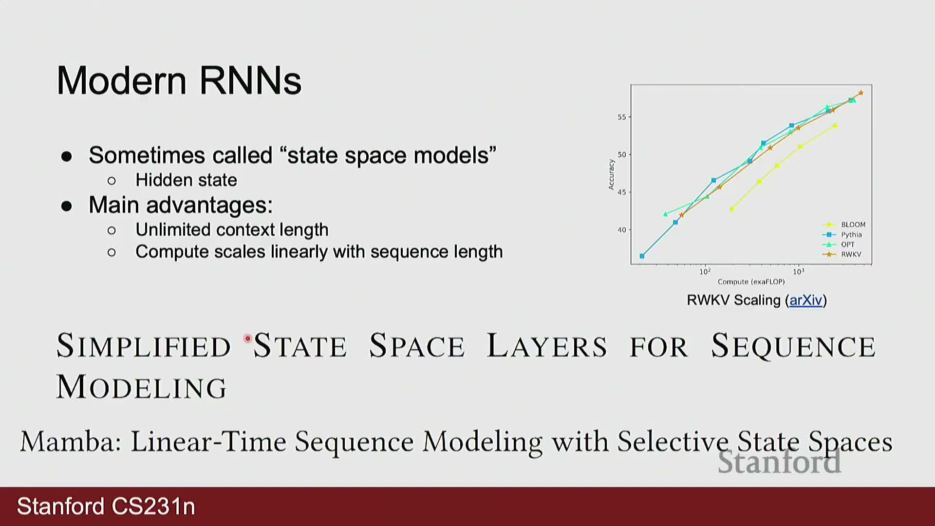
Recent work revives recurrent and state-space approaches to address transformer context and scaling limits
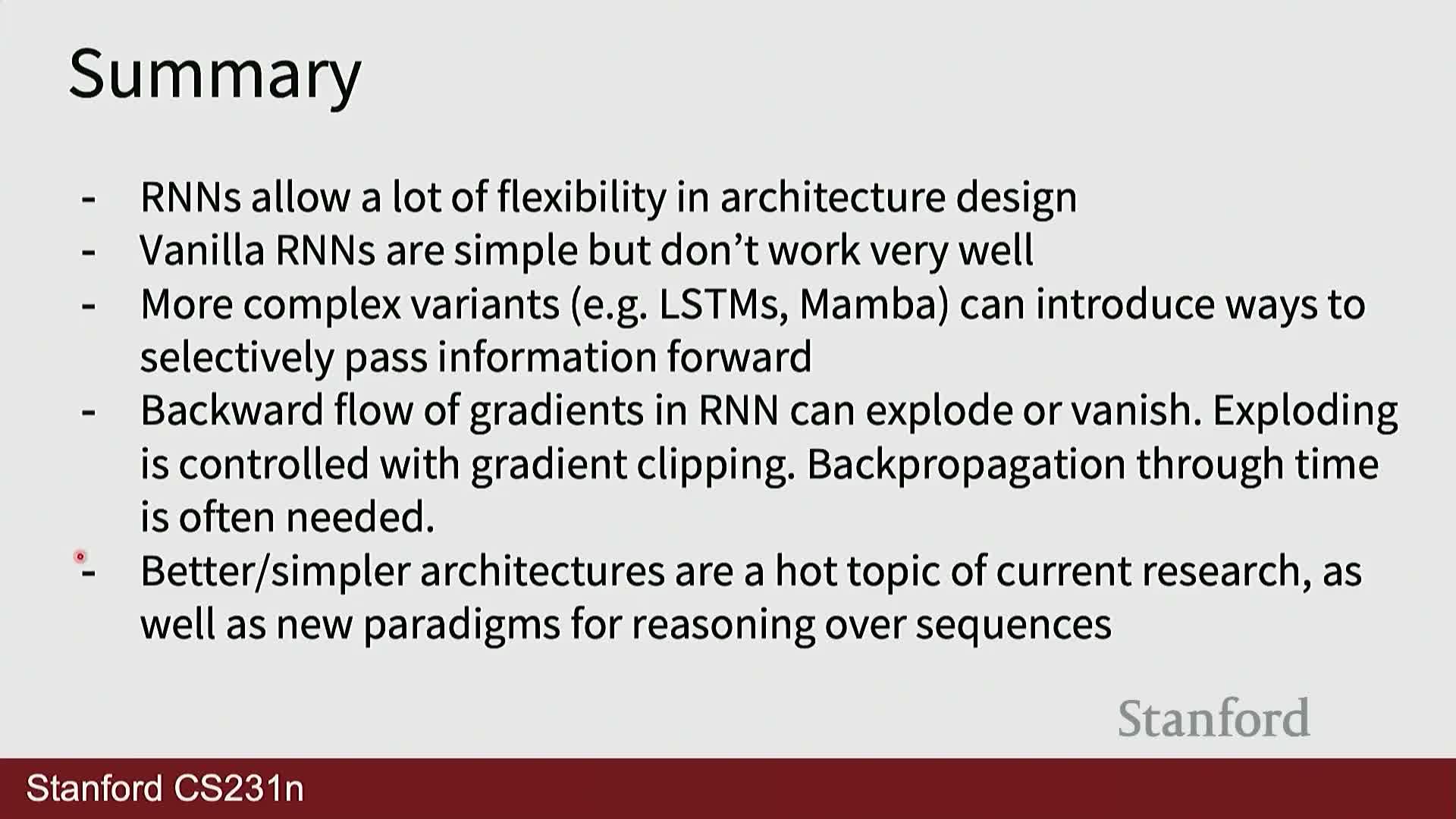
Recent research explores RNN-like and state-space models (for example RWKV and mamba) as alternatives to standard transformers to obtain linear-time sequence processing and practically unbounded context without quadratic attention costs.
- Motivation:
- Transformers impose a fixed maximum context and incur quadratic compute with sequence length, creating scaling bottlenecks for very long-context tasks.
- Goals and trade-offs:
- These models aim to retain the sequential efficiency and arbitrarily long context of recurrent formulations while matching the representational power of attention-based architectures.
- Often they reinterpret recurrence to admit efficient parallel implementations and offer promising compute/memory trade-offs.
As a result, active research seeks to combine the best aspects of recurrence and attention to build scalable long-context models.
Enjoy Reading This Article?
Here are some more articles you might like to read next: