Stanford CS231N | Spring 2025 | Lecture 9- Object Detection, Image Segmentation, Visualizing
- Lecture scope and recap of sequence models and attention
- Vision Transformers convert images to token sequences with positional embeddings and class pooling for classification
- Transformer architectural optimizations improve training stability and expressive power
- Core computer vision tasks comprise classification, detection, segmentation, and model interpretability
- Semantic segmentation assigns a class label to every pixel using context-aware models
- Fully convolutional networks use encoder–decoder topology with downsampling and upsampling to produce dense outputs
- UNet architecture retains encoder spatial features via skip connections to sharpen decoder outputs
- Transpose convolution (deconvolution) provides a learnable upsampling operation for dense prediction
- Instance segmentation differentiates object instances in addition to pixel classes, which motivates object detection
- Sliding-window classification is simple but unscalable; region proposals and RCNN family improved efficiency
- Region Proposal Networks (RPNs) learn to propose candidate object boxes and box refinements
- Single-stage detectors (e.g., YOLO) predict many bounding boxes in a single pass using a dense grid and non-maximum suppression
- DETR (Detection Transformer) formulates detection as a set prediction problem using transformer encoders, decoders, and trainable object queries
- Mask R-CNN extends detection pipelines with per-instance mask prediction to implement instance segmentation
- Visualization and interpretability remain critical for trustworthy computer vision systems
- Saliency maps, CAM, and Grad-CAM provide pixel- and region-level attributions for class predictions
- Transformer attention maps provide direct, interpretable token-to-token and patch-level explanations for vision models
Lecture scope and recap of sequence models and attention
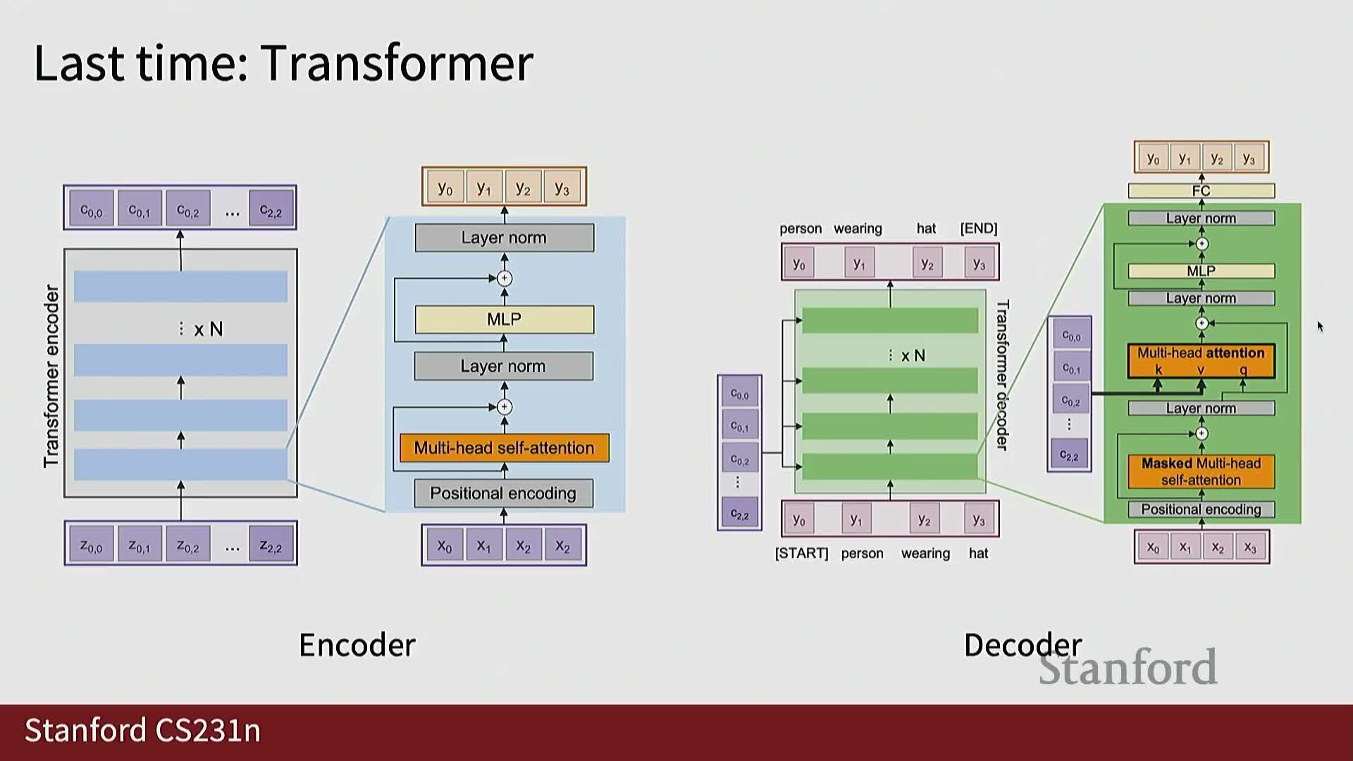
The lecture introduces core computer vision tasks—detection, segmentation, and visualization—and briefly recaps sequence modeling advances that motivate modern architectures.
It summarizes the transition from RNNs and convolutional sequence models to transformer-based models, characterized by:
-
multi-headed self-attention
-
layer normalization
- feedforward (MLP) blocks
The encoder–decoder paradigm is presented as the canonical transformer structure for tasks that require an encoded representation followed by a decoding stage for generation or prediction.
This recap establishes the conceptual foundation for applying transformer ideas to vision tasks later in the lecture.
Vision Transformers convert images to token sequences with positional embeddings and class pooling for classification
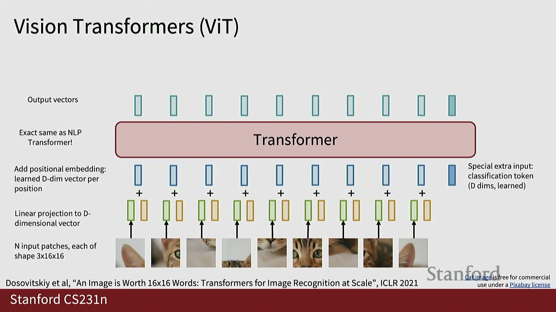
Vision Transformers (ViTs) represent images by splitting them into spatial patches, projecting each patch into a D-dimensional token vector, and treating the resulting sequence with standard transformer encoders.
Key implementation details:
-
Patchification removes explicit 2D location, so positional embeddings are added to restore spatial information:
- 1D sequence-index embeddings, or
- 2D (x,y) encodings
- For image classification, ViTs commonly use a learnable class token whose final representation is projected to a C-dimensional softmax probability vector.
- Alternatively, ViTs may apply global pooling across output tokens before classification.
- Supervision uses standard cross-entropy (softmax) losses and backpropagation.
- Architecturally, ViTs remain compatible with typical transformer components such as multi-head self-attention, layer normalization, and feedforward MLPs.
Transformer architectural optimizations improve training stability and expressive power
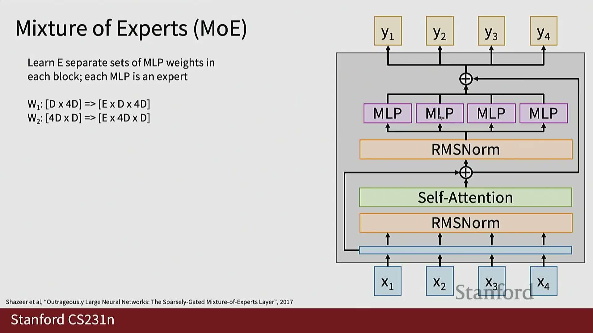
Modern transformer training adopts several empirical and theoretical tweaks to improve stability and capacity.
Important techniques:
-
Pre-layer Residual + LayerNorm (pre-norm)
- Place LayerNorm before self-attention and the MLP to preserve near-identity pathways and retain normalized gradients during learning.
- Place LayerNorm before self-attention and the MLP to preserve near-identity pathways and retain normalized gradients during learning.
-
RMSNorm
- A lightweight normalization alternative that removes mean-centering and can stabilize training for large models.
- A lightweight normalization alternative that removes mean-centering and can stabilize training for large models.
-
Gated MLP variants (e.g., GLU / Gated Linear Units)
- Introduce multiplicative gating between linear projections to increase nonlinearity without proportionally increasing parameters.
- Introduce multiplicative gating between linear projections to increase nonlinearity without proportionally increasing parameters.
-
Mixture-of-Experts (MoE) layers
- Use a learned router to dispatch tokens to a small subset of expert subnetworks, enabling very large parameter counts with sparse compute per token.
- Use a learned router to dispatch tokens to a small subset of expert subnetworks, enabling very large parameter counts with sparse compute per token.
These techniques are widely used in large language models and vision architectures to balance trainability, capacity, and inference cost.
Core computer vision tasks comprise classification, detection, segmentation, and model interpretability
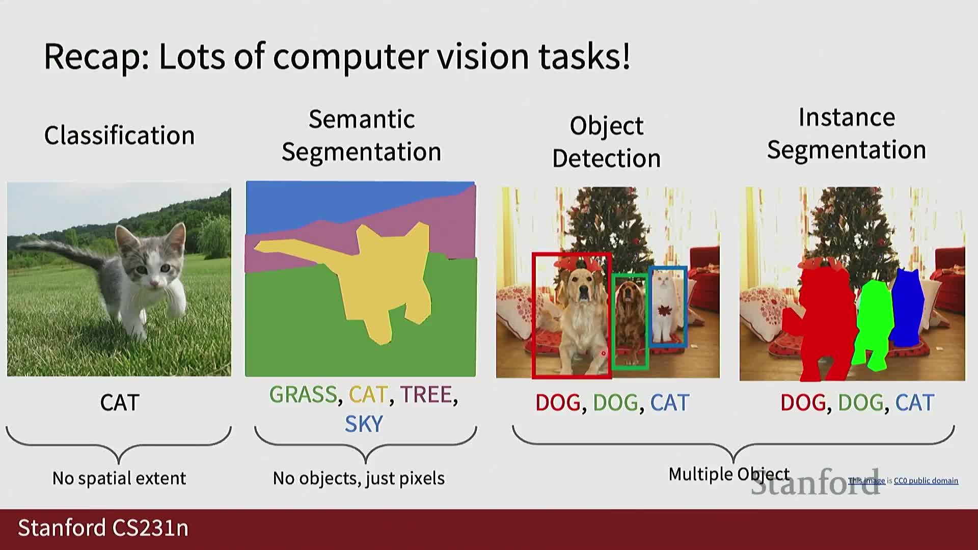
Computer vision is organized into canonical tasks:
-
Image-level classification
-
Object detection
-
Semantic and instance segmentation
-
Visualization / understanding to interpret model decisions
Each task imposes distinct output structures and evaluation requirements:
-
Semantic segmentation requires pixelwise label maps.
-
Instance segmentation requires per-instance masks and bounding boxes.
Visualization and interpretability are critical in high-stakes domains (e.g., medical imaging) because end-users need localized explanations (both where and why) in addition to categorical predictions.
Understanding these tasks and their data/annotation needs is essential when designing models or choosing architectures for applied systems.
Semantic segmentation assigns a class label to every pixel using context-aware models
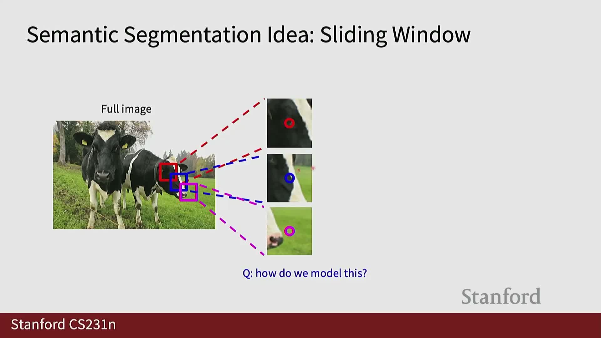
Semantic segmentation maps each pixel in an image to a semantic class label, which requires modeling both local and contextual information because isolated pixel values are ambiguous.
Practical modeling choices:
- Use convolutional neural networks or modern alternatives (e.g., ViTs) that consume image patches or the whole image and output a dense label map.
- Supervise per-pixel classification with a pixelwise loss such as cross-entropy aggregated over image pixels.
- Naïvely running a full network per pixel is infeasible, so segmentation architectures produce the entire label map in a single forward pass using fully convolutional designs that preserve spatial structure across layers.
Training requires pixel-level ground-truth label maps and substantial annotation effort, though contemporary datasets and annotation tools alleviate some labeling costs.
Fully convolutional networks use encoder–decoder topology with downsampling and upsampling to produce dense outputs
Fully convolutional networks (FCNs) downsample spatial resolution to increase receptive field and channel capacity, then upsample back to image resolution to emit dense predictions.
Downsampling methods:
-
Strided convolutions
-
Pooling (max/average)
Upsampling methods:
- Non-learned schemes: nearest-neighbor, saved max-pool indices
- Learned operators: transpose convolutions, learned upsampling filters that expand resolution while enabling parameterized reconstruction
Learned upsampling:
- Apply trainable kernels to low-resolution activations.
- Sum overlapping outputs at higher-resolution locations (differentiable and trainable end-to-end).
The overall training objective typically sums per-pixel classification losses across the output map, enabling gradient-based learning of both encoder and decoder parameters.
UNet architecture retains encoder spatial features via skip connections to sharpen decoder outputs
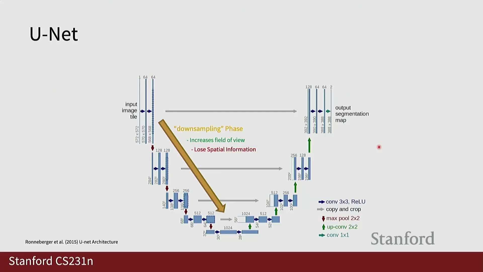
The U-shaped architecture (UNet) contains:
- A contraction path that downscales spatial resolution and expands channel depth.
- An expansion path that upsamples back to the original resolution.
Crucial design element:
-
Skip connections copy encoder feature maps to corresponding decoder layers to preserve fine-grained spatial structure lost during downsampling.
Benefits and implementation:
- Lateral connections improve boundary localization and produce sharper segmentation masks—important for tasks like medical image segmentation.
- UNet variants typically use concatenation or addition of encoder features at each decoder step and apply convolutional blocks to refine the combined information.
Because of this design, UNets remain strong baselines for many segmentation tasks where large pre-trained foundation models are not used.
Transpose convolution (deconvolution) provides a learnable upsampling operation for dense prediction
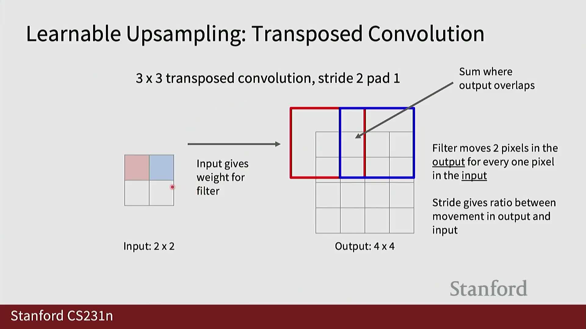
Transpose convolution performs convolution-like operations while treating the layer as the spatial inverse of a standard convolution, producing larger output spatial dimensions from lower-resolution inputs.
Key properties:
- Maintains learnable filters like ordinary convolutions.
- Produces overlapping receptive-field contributions that are summed at overlapping output locations, enabling learned reconstruction during upsampling.
- Can be implemented as a convolution with appropriately strided and padded inputs or explicitly as the matrix-transpose equivalent of standard convolution.
As a trainable decoder primitive, transpose convolutions integrate seamlessly into FCNs and UNet-style decoders to produce high-resolution, learned predictions.
Instance segmentation differentiates object instances in addition to pixel classes, which motivates object detection
Instance segmentation extends semantic segmentation by assigning pixels both a class label and an instance identifier, enabling the model to distinguish multiple occurrences of the same category.
Key implications:
- Requires object-centric reasoning—detecting object candidates (e.g., bounding boxes) and then predicting per-instance masks—because pixelwise semantic labels alone do not indicate instance membership.
- Typical pipeline:
- Use an object detection system to output class probabilities and bounding box coordinates (x,y,width,height).
- Combine boxes with mask prediction heads to yield instance-level masks.
- Use an object detection system to output class probabilities and bounding box coordinates (x,y,width,height).
- Training uses multi-task objectives (classification loss plus regression loss for box coordinates) to supervise both class and spatial localization.
Sliding-window classification is simple but unscalable; region proposals and RCNN family improved efficiency
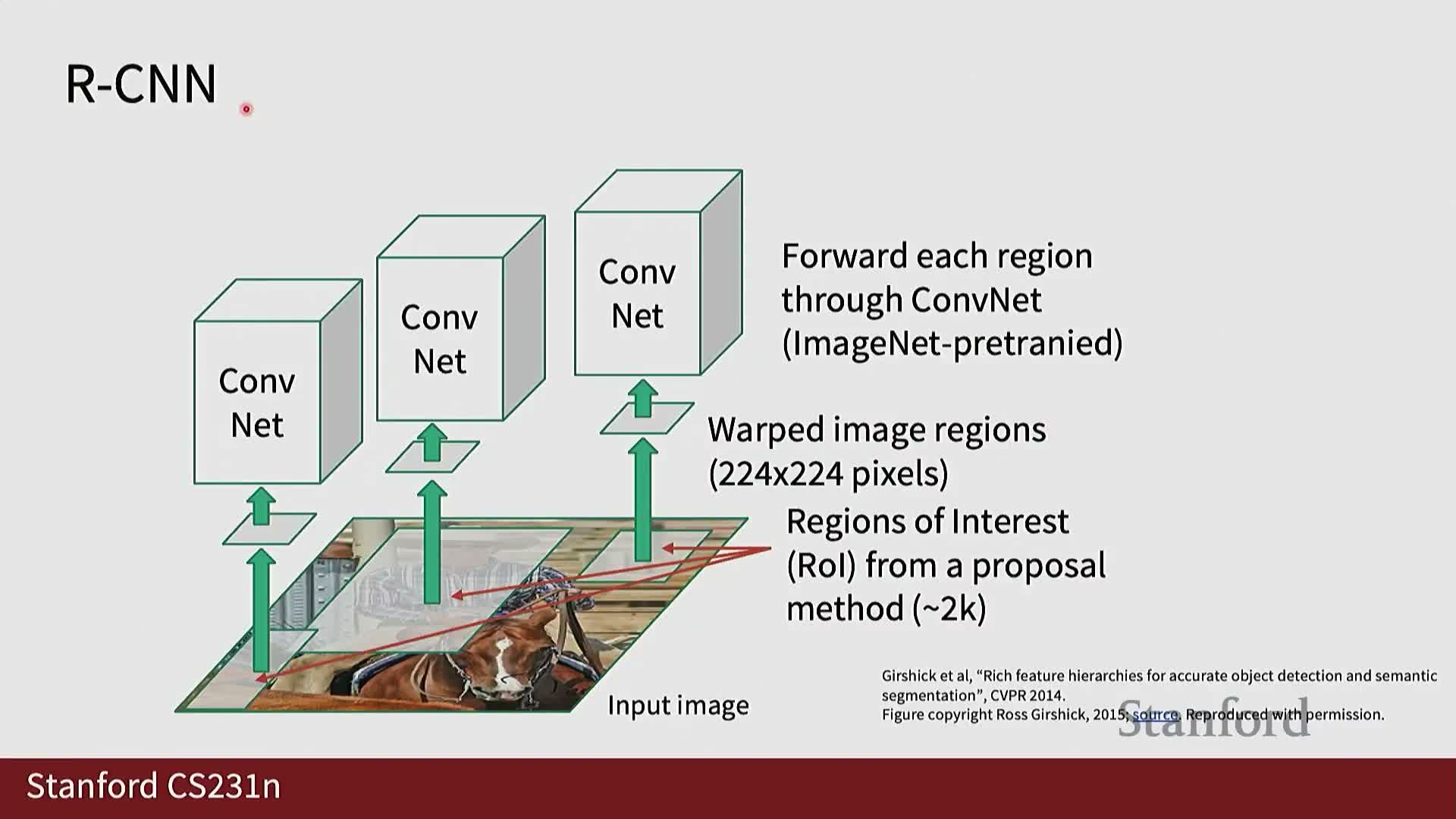
A brute-force sliding-window approach classifies a dense set of candidate windows, but enumerating all spatial locations and scales is computationally prohibitive.
Region proposal methods address this by generating a smaller set of likely object-containing regions that downstream classifiers refine and score. Historical pipeline evolution:
-
RCNN-style: crop proposals and run a full CNN per proposal—accurate but slow.
-
Faster variants: process the whole image once with a CNN to produce a shared feature map, then extract region features from that map for proposal refinement and classification—reduces redundant computation significantly.
These approaches separate region proposal generation from per-region classification/regression; later work unified many steps for additional efficiency improvements.
Region Proposal Networks (RPNs) learn to propose candidate object boxes and box refinements
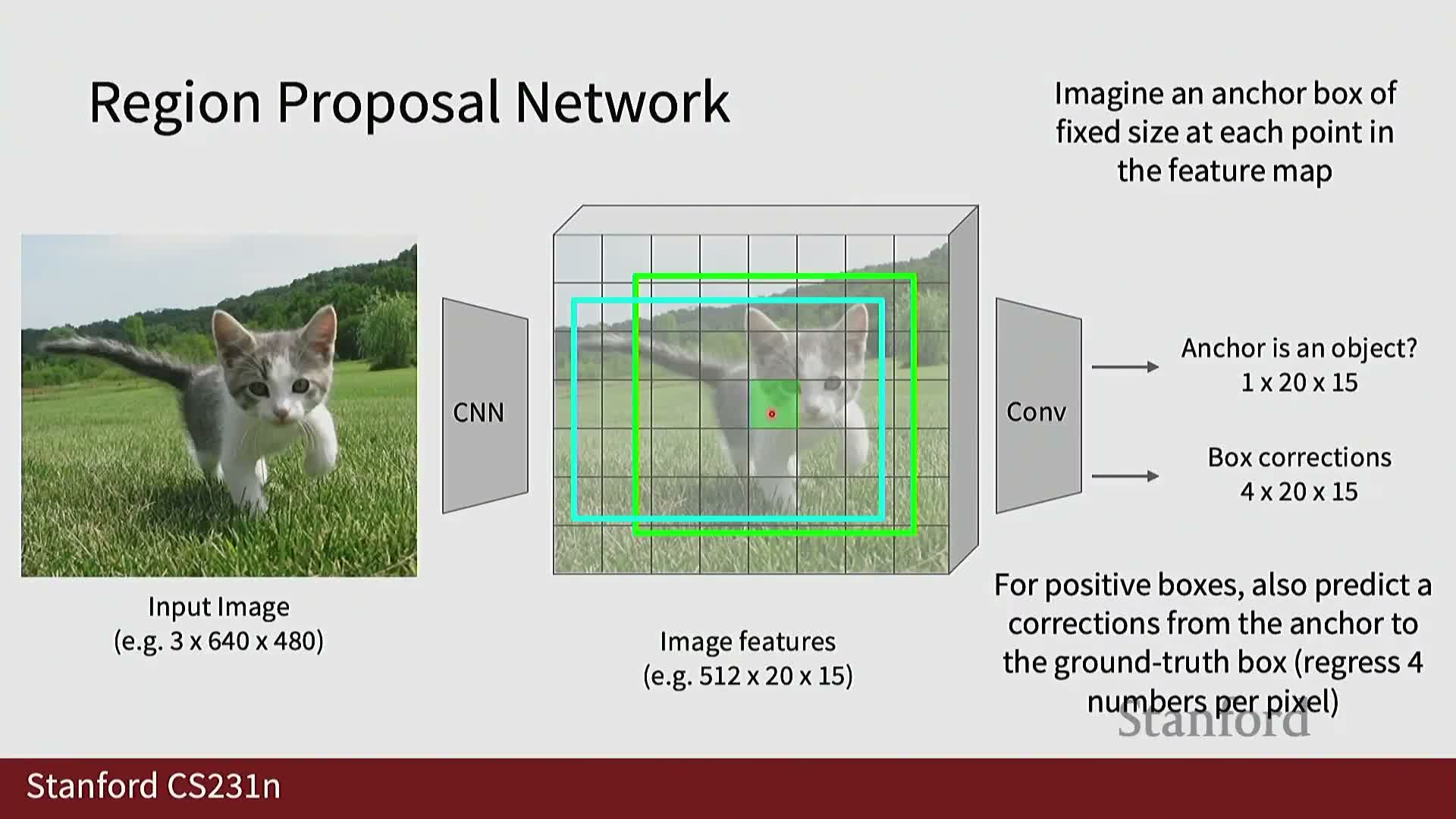
Region Proposal Networks (RPNs) embed a lightweight network atop convolutional feature maps to predict objectness scores and refined bounding box offsets for a set of predefined anchors across the image.
Training and inference details:
- Supervised with annotated box locations: positive anchors near ground-truth objects are regressed toward ground-truth coordinates while negatives are suppressed.
- At inference, proposals are ranked by objectness score and the top-k proposals are selected for downstream classification and refinement.
- RPNs replaced expensive hand-crafted region proposal pipelines and enabled efficient two-stage detectors such as Faster R-CNN.
Single-stage detectors (e.g., YOLO) predict many bounding boxes in a single pass using a dense grid and non-maximum suppression
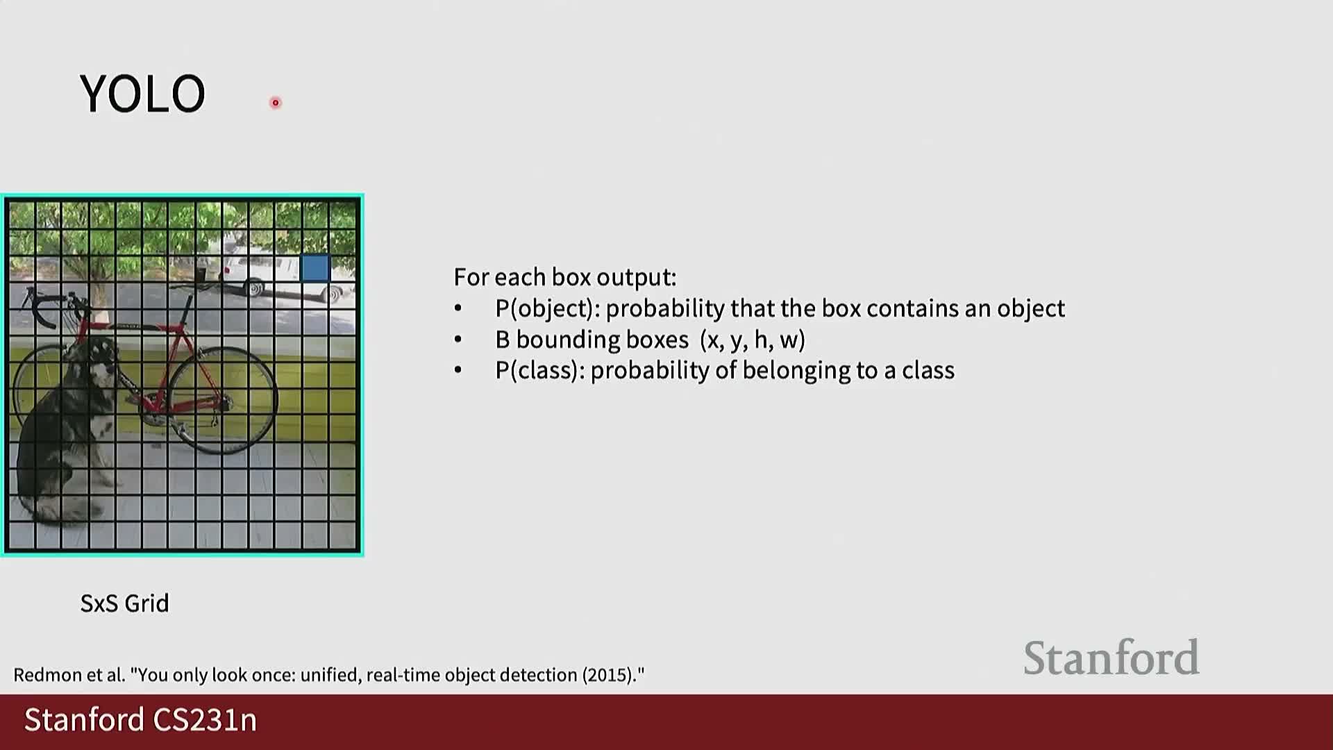
Single-stage detectors divide the image into an SxS grid and predict a fixed number B of proposed bounding boxes per cell along with class probability vectors and confidence scores, producing all candidate boxes in one forward pass.
Characteristics:
- Each predicted box includes coordinates and class probabilities.
- Post-processing such as confidence thresholding and non-maximum suppression (NMS) prunes redundant, overlapping detections to yield final object locations.
- Architectures like YOLO are optimized for speed using a single fully convolutional network and are widely used for real-time detection.
- Hyperparameters (grid size S, boxes per cell B) determine localization granularity and capacity, while NMS settings affect precision/recall trade-offs.
DETR (Detection Transformer) formulates detection as a set prediction problem using transformer encoders, decoders, and trainable object queries
DETR uses a transformer encoder to process image-derived tokens (patch embeddings or CNN features with positional encodings) and a transformer decoder that consumes a fixed set of learned query vectors to produce a set of object predictions.
How DETR works:
- The encoder produces contextualized token representations from image features.
- A fixed set of learned query vectors is input to the decoder; each query asks the model to predict one object.
- Decoder outputs are passed through small feedforward networks to regress bounding boxes and predict class labels (including a no-object class).
- Training uses a bipartite matching loss between predicted set elements and ground-truth objects to supervise the unordered set prediction.
Cross-attention between queries and encoder outputs lets the decoder localize and classify objects without explicit proposal mechanisms. DETR’s canonical formulation eliminates hand-designed NMS by learning set-level outputs, though practical variants modify training and architecture to improve convergence and performance.
Mask R-CNN extends detection pipelines with per-instance mask prediction to implement instance segmentation
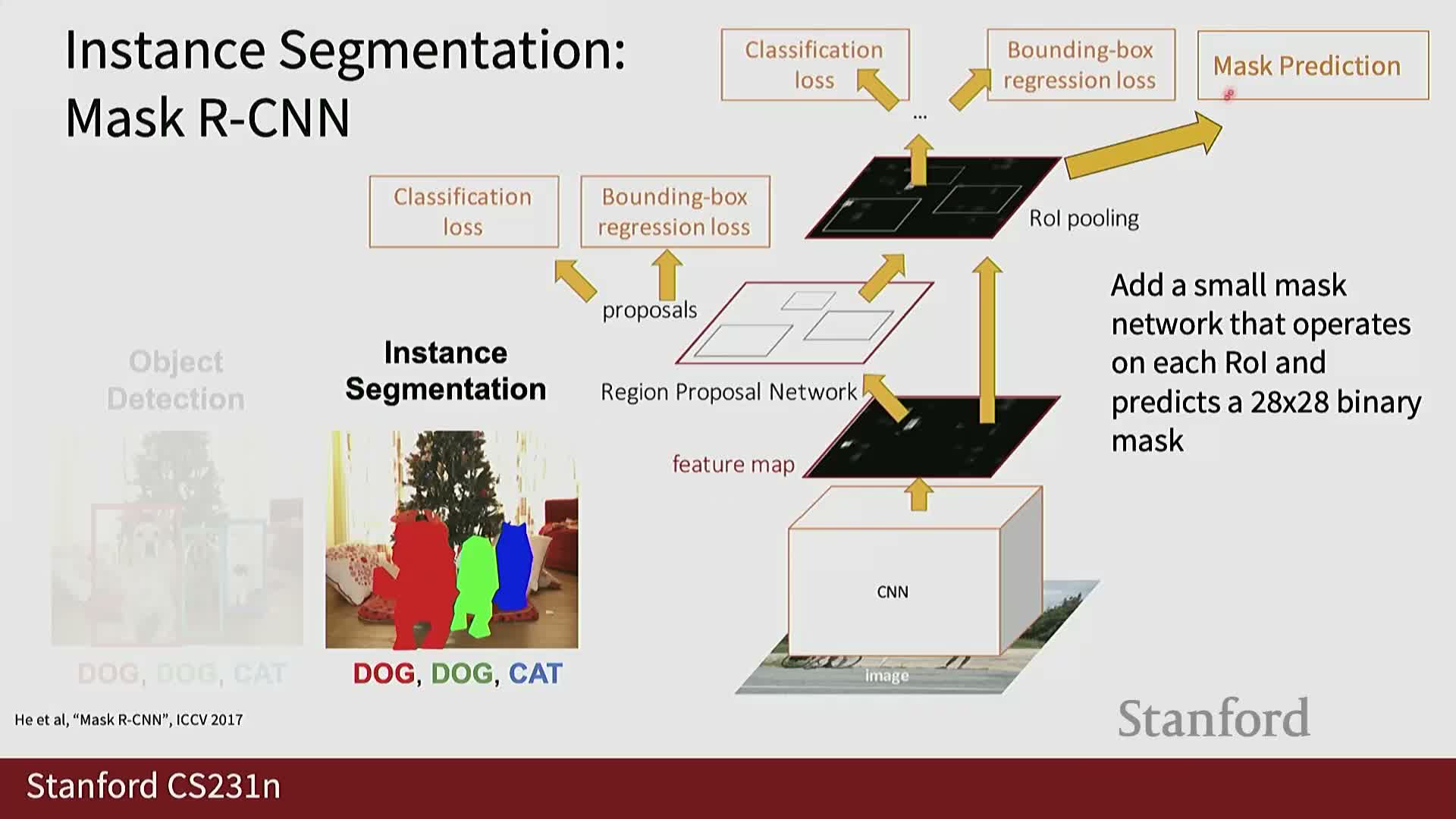
Mask R-CNN augments a two-stage detection pipeline by adding a parallel mask head that predicts a binary segmentation mask for each detected bounding box while simultaneously classifying the object and refining box coordinates.
Pipeline details:
- After region features are pooled for each proposal, separate branches predict:
-
Class scores
-
Bounding-box refinements
- A small-resolution mask (typically upsampled to the box size)
-
Class scores
- The mask branch is a small fully convolutional network trained with per-pixel binary cross-entropy against the instance mask.
This multitask formulation yields high-quality instance masks and remains a foundational, interpretable approach for precise per-instance segmentation. Many open-source APIs provide Mask R-CNN implementations for applied use.
Visualization and interpretability remain critical for trustworthy computer vision systems
Model visualization techniques reveal what representations and decisions networks encode, which is essential for debugging, trust, and deployment in high-stakes domains (e.g., medical imaging).
Common approaches:
- Visualize learned filters and activation patterns in early convolutional layers.
- Compute saliency maps that quantify sensitivity of class scores to pixel perturbations, producing localized importance heatmaps.
These techniques help assess whether models rely on semantically meaningful signals or spurious correlations, and they guide model redesign, targeted data collection, or trust calibration for deployed systems.
Saliency maps, CAM, and Grad-CAM provide pixel- and region-level attributions for class predictions
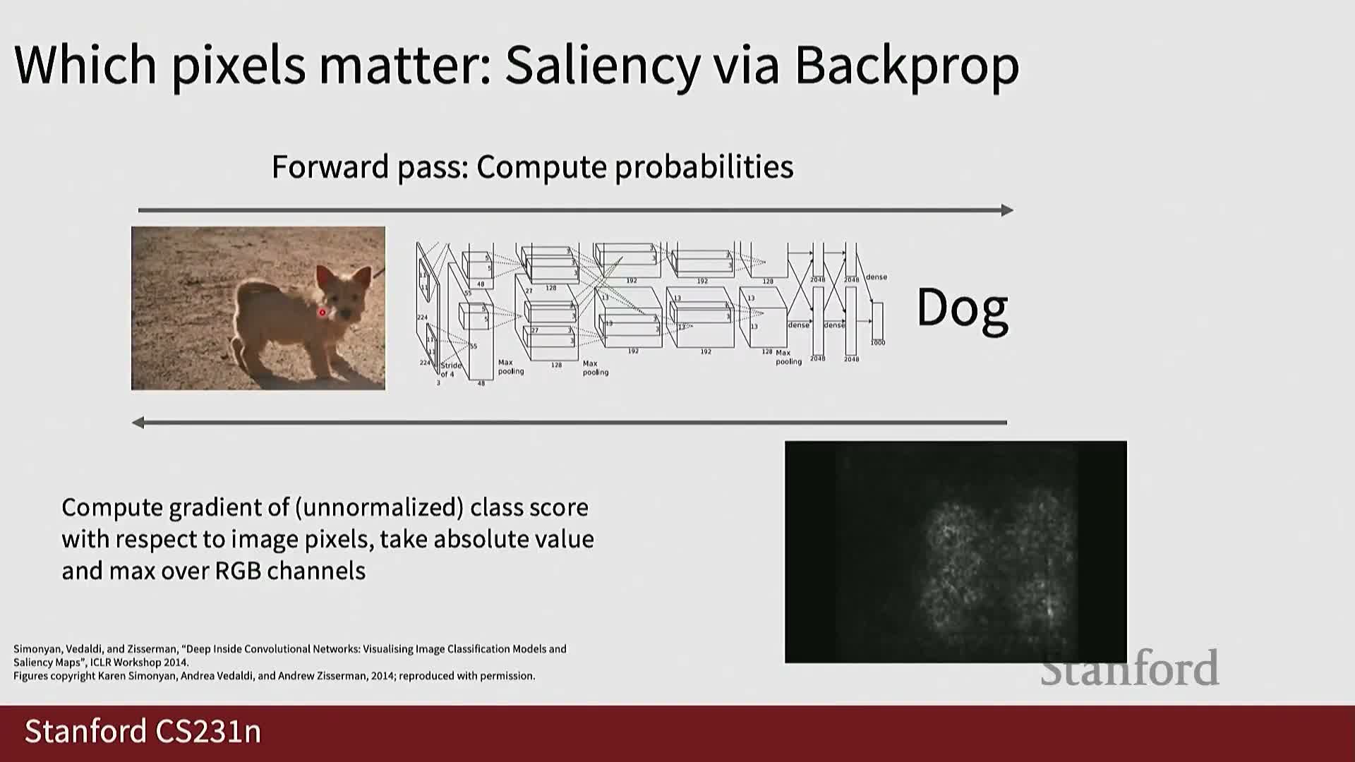
Saliency and class-discriminative localization methods:
-
Saliency maps compute the gradient of a class score with respect to input pixels; the gradient magnitude highlights pixels where small changes would strongly affect the predicted class.
-
Class Activation Mapping (CAM) constructs class-specific localization maps by linearly combining convolutional feature maps with classifier weights to reveal discriminative regions—but CAM originally requires a global pooling-based architecture at the end.
-
Grad-CAM generalizes CAM by weighting feature maps with the spatial average of gradients flowing into a chosen convolutional layer, producing class-discriminative localization heatmaps for a wider range of architectures; positive-only activations (ReLU) are often used to focus on supporting evidence.
These methods are practical diagnostic tools and produce human-interpretable visual explanations, though they approximate attribution and should be used with awareness of their assumptions.
Transformer attention maps provide direct, interpretable token-to-token and patch-level explanations for vision models
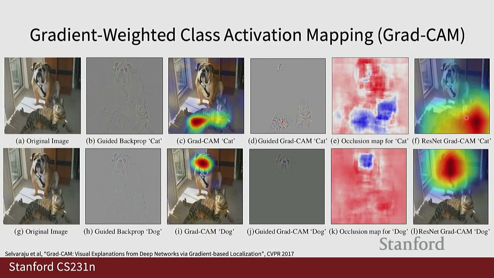
Transformer-based vision models naturally produce attention weight matrices that quantify how each output token attends to input tokens or image patches, enabling direct visualization of spatial attention patterns across layers and heads.
Interpretability advantages:
- Attention maps can be inspected per head/layer or aggregated to show which image regions contribute to a particular output token or predicted class.
- Cross-attention summaries facilitate tracing model decisions back to specific image patches, offering a more transparent mechanism for attribution compared to many gradient-based methods in CNNs.
- Because attention operates over discrete tokens with positional encodings, transformer-based explanations align naturally with image patches and are thus especially useful for debugging and understanding model behavior in practical applications.
Enjoy Reading This Article?
Here are some more articles you might like to read next: