Stanford CS231N Deep Learning for Computer Vision | Spring 2025 | Lecture 10- Video Understanding
- Course introduction and guest lecturer announcement
- Motivation for multi‑sensory machine intelligence and course focus on vision
- Definition of video as images plus time and the video classification problem
- Key differences between image and video tasks and data scale challenges
- Temporal and spatial downsampling and clip‑based training for tractability
- Per‑frame image classifier baseline and frame sampling strategies
- Late fusion: concatenation and pooling of per‑frame features
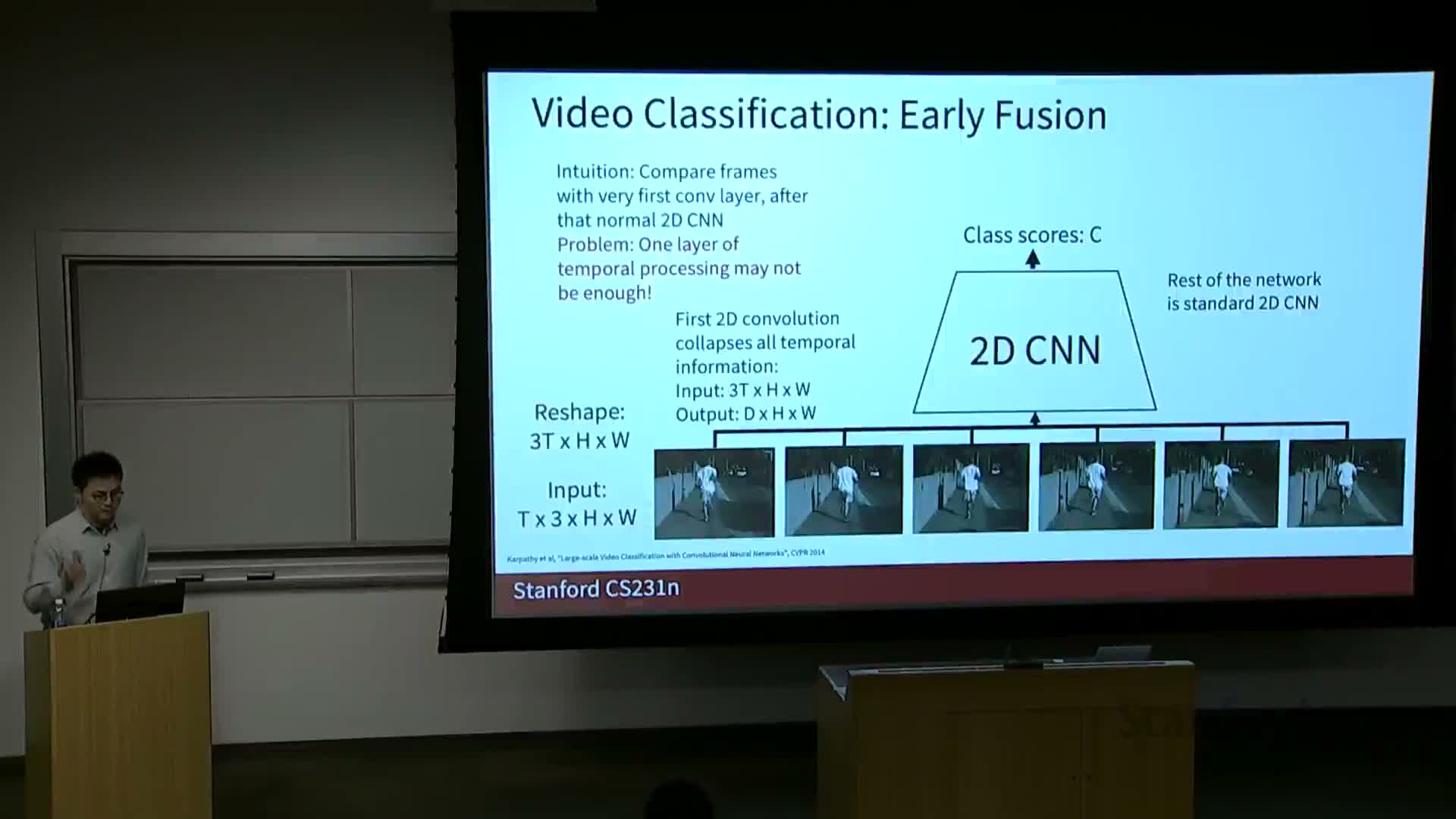
- Early fusion: collapsing temporal channels at input and limitations
- Slow fusion idea and introduction to 3D convolutions
- 3D convolutional operations and tensor dimensions
- Toy comparison of late fusion, early fusion and 3D CNN receptive fields
- Temporal shift invariance and representational efficiency of 3D kernels
- Visualization of 3D convolutional filters and qualitative interpretations
- Sports1M dataset and coarse empirical findings on fusion strategies
- Practical dataset distribution issues and C3D origin story
- Clip length conventions and computational cost of 3D CNNs
- Motivation to treat space and time separately and optical flow fundamentals
- Two‑stream networks combining appearance and motion streams
- Modeling long‑term temporal structure with recurrent models
- Recurrent convolutional networks as spatio‑temporal hybrids
- Non‑local/self‑attention blocks for spatio‑temporal interaction
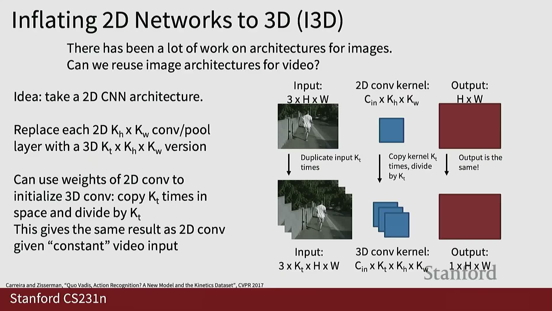
- I3D inflation: transferring 2D architectures and weights to 3D
- Progress in video architectures and large‑scale performance gains
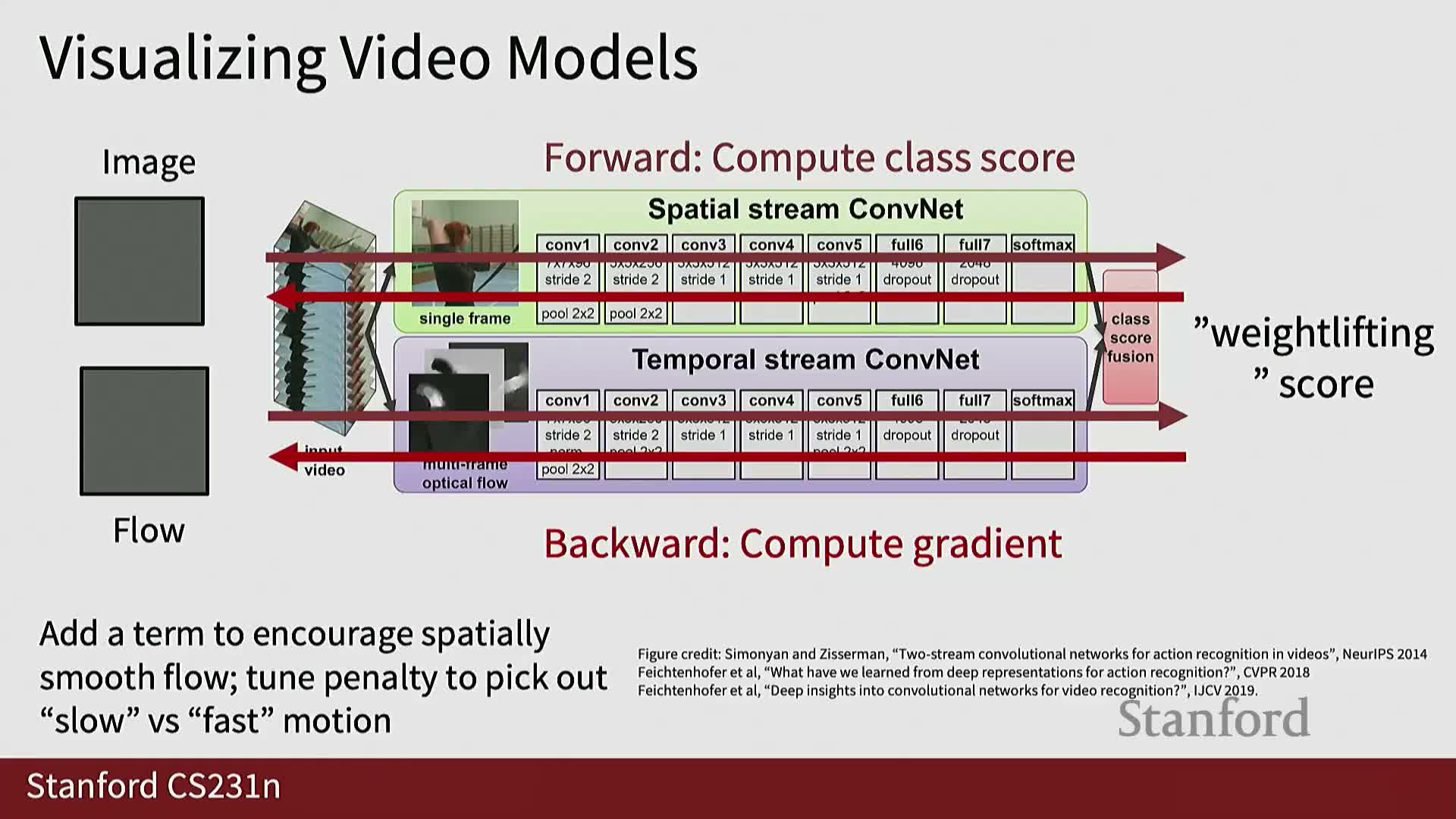
- Visualization via class‑score optimization for appearance and flow streams
- Temporal action localization and spatio‑temporal detection tasks
- Audio‑visual multimodal tasks and visually‑guided source separation
- Efficiency strategies: clip selection, modality selection and policy learning
- Egocentric multimodal video streams and social interaction understanding
- Connecting video understanding with large language models and video foundation models
Course introduction and guest lecturer announcement
Introduces the guest lecture format and presents the guest lecturer’s affiliation and research focus to establish the session context for deep learning approaches to multi‑sensory and visual problems.
The opening frames who is speaking, where they work, and the high‑level questions the lecture will address—setting expectations for the material and technical depth to follow.
Motivation for multi‑sensory machine intelligence and course focus on vision
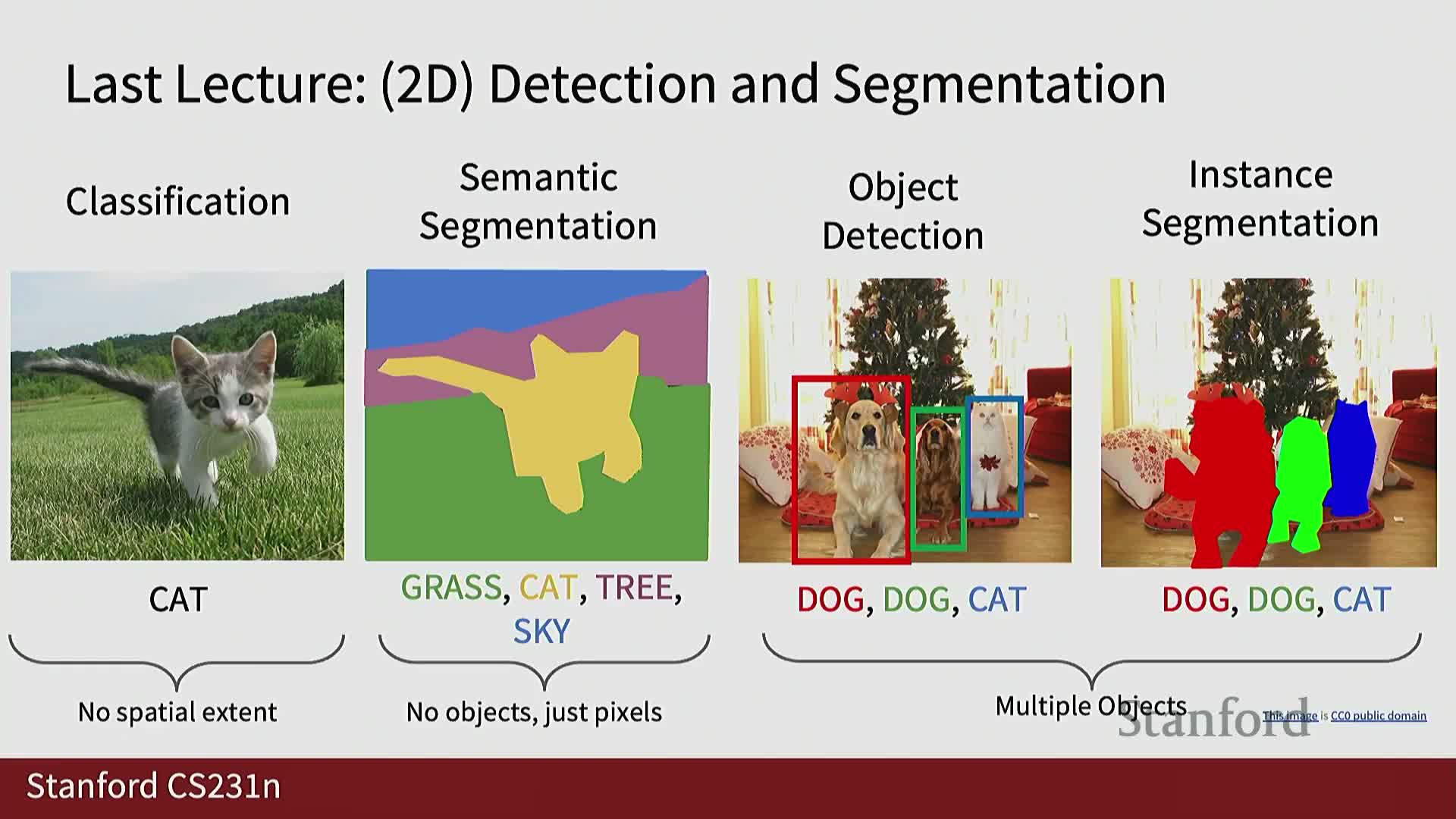
Frames the research interest in combining visual data with other sensory modalities such as audio and tactile signals, and emphasizes that the lecture will focus on video understanding as an extension of the image‑based tasks covered earlier in the course.
Key emphasis:
- Combining modalities to capture complementary information (e.g., appearance + sound).
- Treating video as a natural next step after image tasks, with additional temporal complexity to consider.
Definition of video as images plus time and the video classification problem
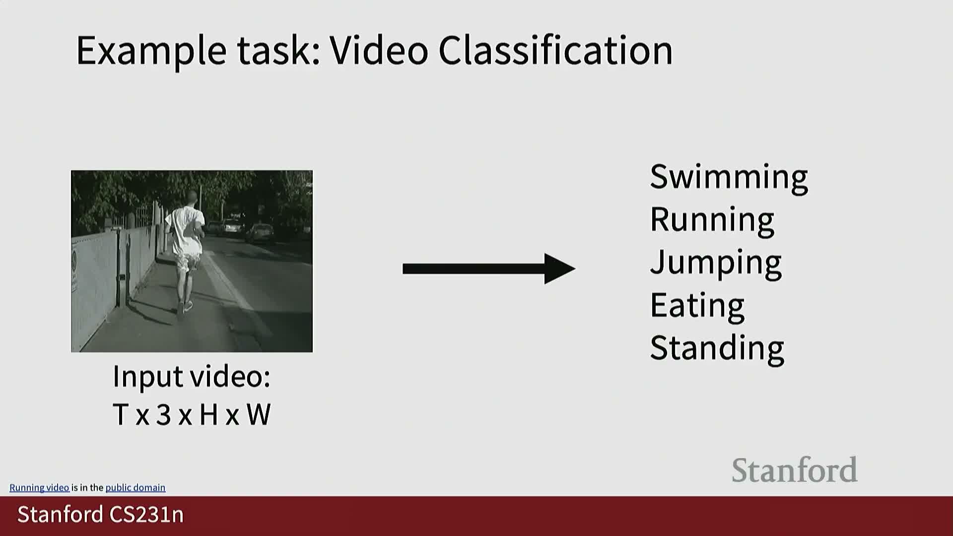
Video is defined as a temporal sequence of 2D image frames that together form a 4D tensor with shape C×T×H×W (channels, time, height, width).
Video classification is formalized as a mapping from these temporal streams of frames to discrete action or event labels, trained with loss functions such as cross‑entropy, analogous to image classification but applied over time.
Key differences between image and video tasks and data scale challenges
Video tasks typically prioritize activities and temporal dynamics rather than static object appearance.
Practical challenges:
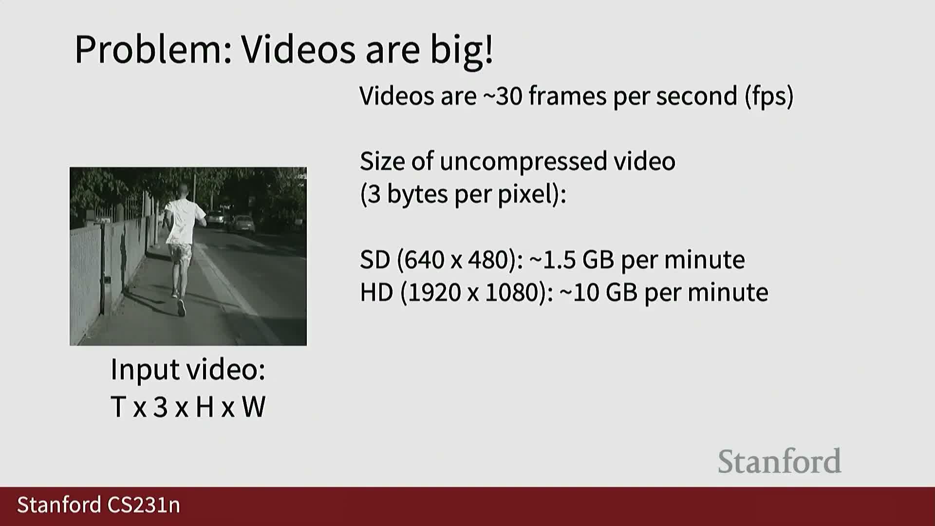
- Videos combine large spatial and temporal resolution, increasing data size.
- High frame rates and resolutions can lead to gigabytes per minute of storage for raw video.
- These scale factors complicate training and impose strict GPU memory and compute constraints.
Temporal and spatial downsampling and clip‑based training for tractability
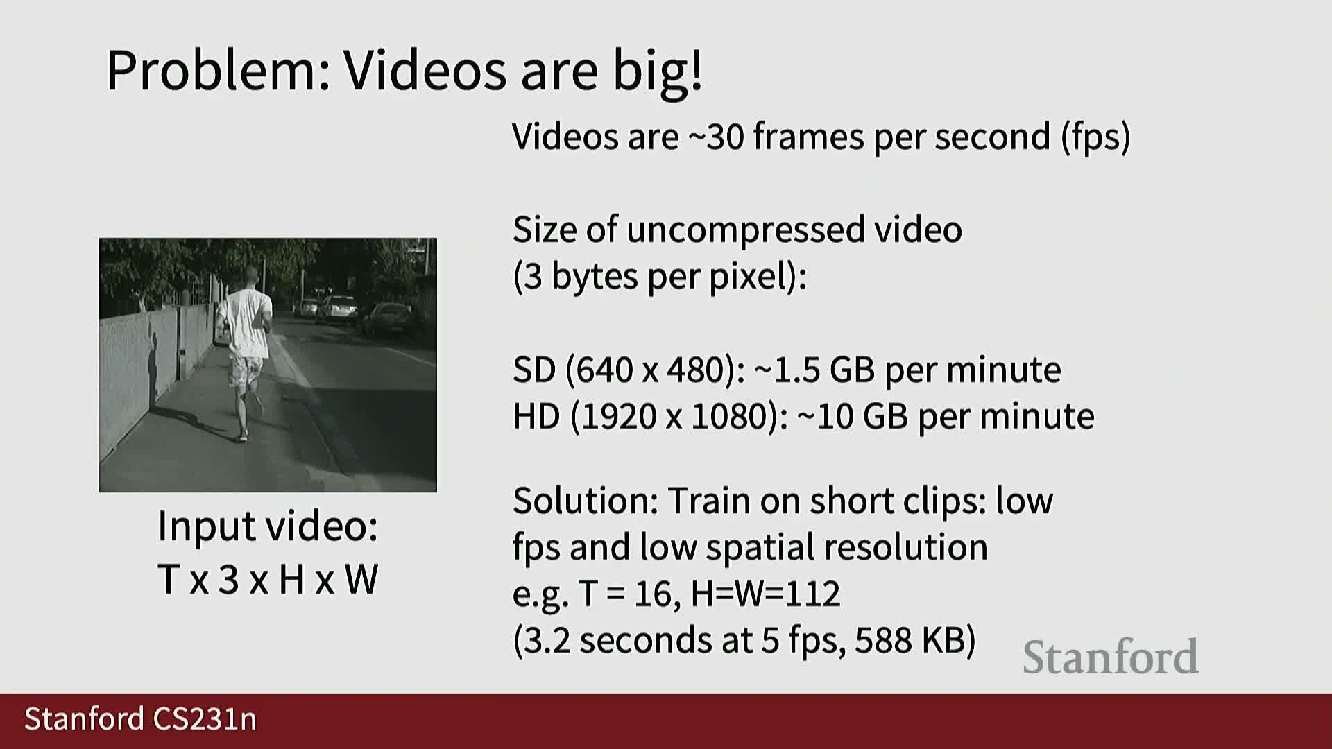
Standard preprocessing strategies make video processing tractable:
-
Reduce spatial resolution (resize frames).
-
Subsample frames per second (lower temporal sampling rate).
-
Train on shorter, fixed‑length clips sampled from the full video (often via sliding windows).
Inference typically proceeds by running the classifier on multiple sampled clips from a video and averaging or otherwise aggregating clip‑level predictions to produce a video‑level label.
Per‑frame image classifier baseline and frame sampling strategies
A simple but strong baseline is the per‑frame approach:
- Apply a standard image CNN to sampled frames independently.
- Aggregate per‑frame predictions (e.g., average scores) to obtain a video prediction.
Sampling strategies matter and remain an active research area:
-
Random sampling vs. adaptive sampling that aims to select the most informative frames from long videos.
Late fusion: concatenation and pooling of per‑frame features
Late fusion approaches:
- Independently extract features per frame using a 2D CNN.
- Aggregate frame features by concatenation or pooling, then train fully‑connected layers or a classifier on the combined vector.
Tradeoffs:
-
Concatenation can cause a parameter explosion as temporal extent grows.
-
Pooling (mean/max) reduces parameters but can lose temporal ordering and fine‑grained dynamics.
Early fusion: collapsing temporal channels at input and limitations
Early fusion concatenates temporal frames along the channel axis and applies 2D convolutions at the network input to collapse temporal information immediately.
Pros and cons:
- Enables immediate mixing of temporal information at the first layer.
- Risks losing structured temporal modeling because it attempts to capture motion in a single early layer rather than across depth.
Slow fusion idea and introduction to 3D convolutions
Slow fusion is an intermediate strategy that gradually fuses temporal and spatial information across network layers using 3D convolutions and 3D pooling.
Rather than collapsing time early or only at the end, slow fusion distributes temporal aggregation across the network depth, allowing hierarchical spatio‑temporal feature learning.
3D convolutional operations and tensor dimensions
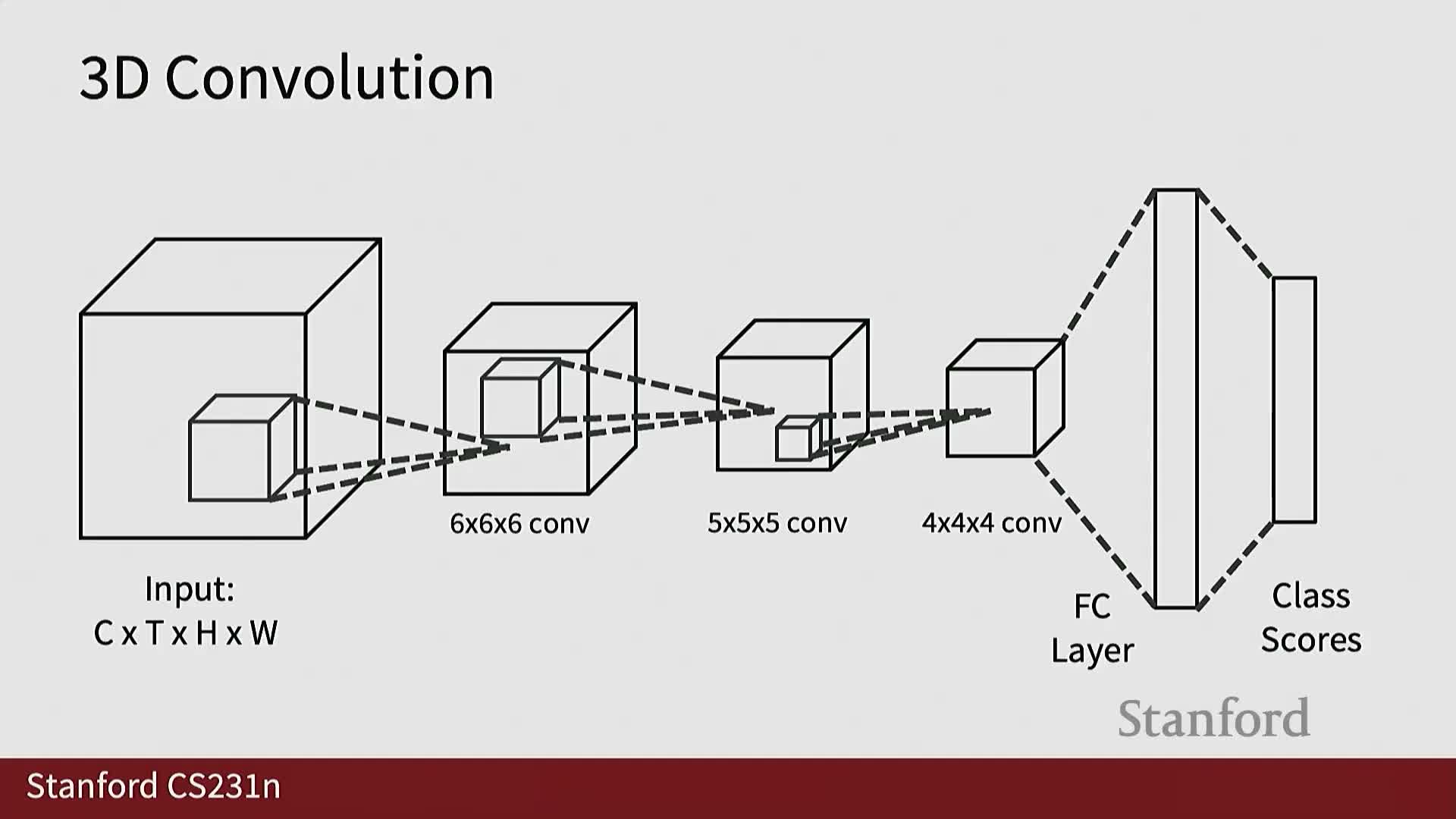
3D convolution (for input tensors shaped C×T×H×W) uses kernels that span both time and space with size kT×kH×kW.
Behavior and benefits:
- Kernels slide over the spatio‑temporal cube to produce feature maps that jointly model local temporal and spatial patterns.
- Channel interactions are preserved across the convolution operations, enabling richer spatio‑temporal filters than stacked 2D operations alone.
Toy comparison of late fusion, early fusion and 3D CNN receptive fields
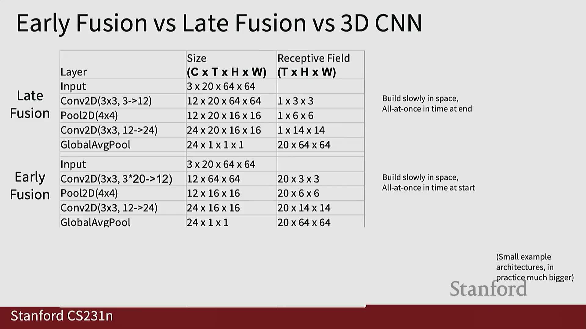
Toy architectures illustrate the differences:
-
Late fusion: preserves temporal extent through the network and aggregates near the end.
-
Early fusion: collapses temporal information in the first layer via channel concatenation.
-
3D CNNs (slow fusion style): incrementally expand both spatial and temporal receptive fields via successive 3D convolutions and pooling, enabling hierarchical motion modeling.
Temporal shift invariance and representational efficiency of 3D kernels
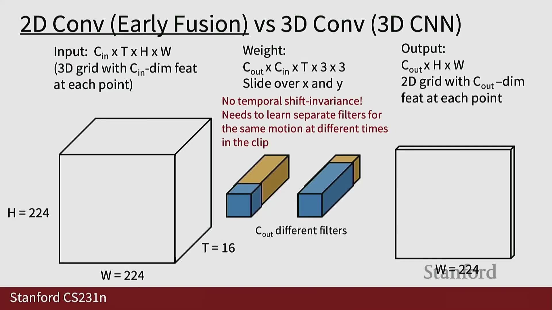
Why 2D kernels that extend fully in time can be problematic:
- A 2D kernel that spans the entire temporal axis lacks temporal shift invariance—it must learn separate filters to model the same temporal pattern at different time positions.
By contrast, 3D kernels that are local in time and slide along T provide temporal translation invariance, making them more parameter‑efficient for modeling repeated motion patterns across time.
Visualization of 3D convolutional filters and qualitative interpretations
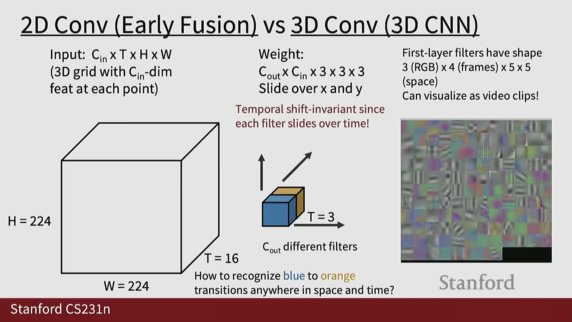
Learned 3D convolution kernels can be visualized as short video clips:
- Visualizations reveal spatio‑temporal patterns such as color transitions, moving edges, and directional motion filters.
- These visualizations help interpret how networks capture motion cues at different depths and scales.
Sports1M dataset and coarse empirical findings on fusion strategies
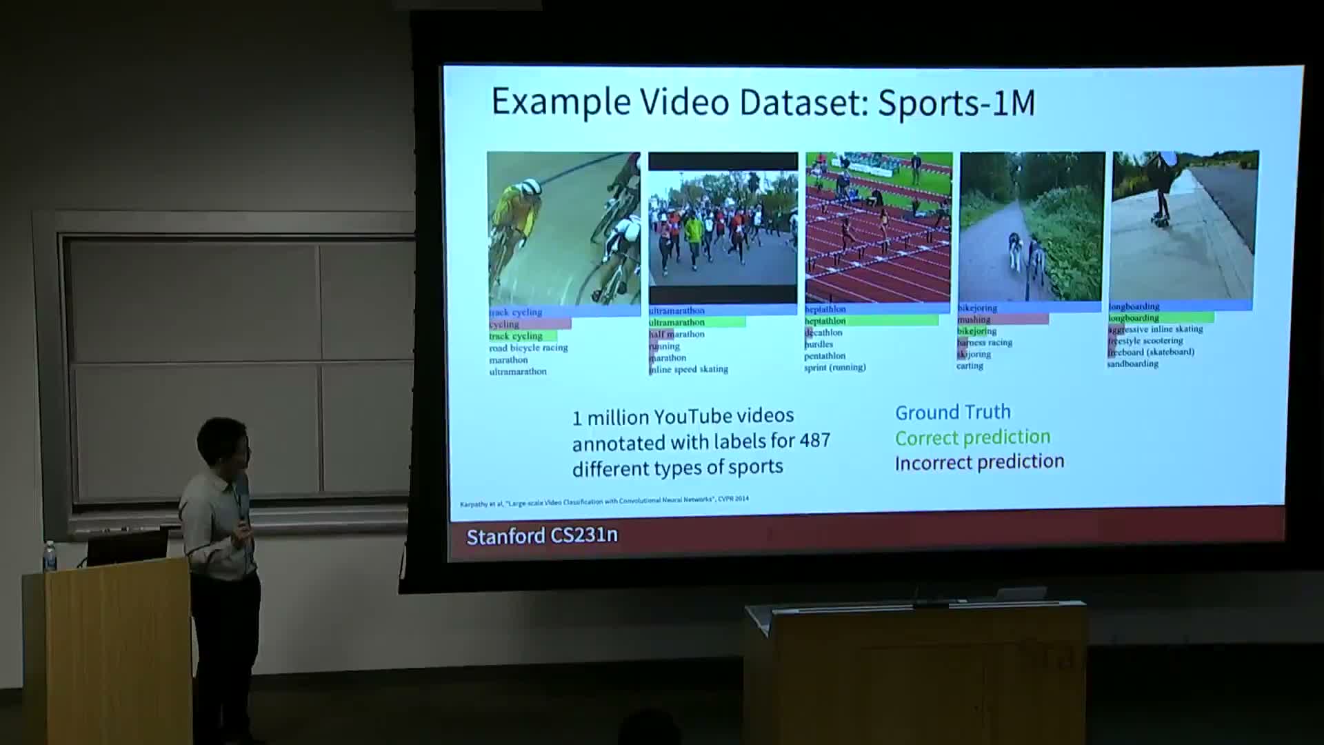
Sports1M is a large, fine‑grained action recognition dataset with hundreds of sports classes.
Empirical findings from early large‑scale studies:
-
Single‑frame baselines are surprisingly strong.
-
Early fusion can perform worse in some settings.
-
Late fusion often yields slight improvements over per‑frame baselines.
-
3D convolutional architectures typically provide modest gains on top of strong per‑frame baselines, depending on compute and data scale.
Practical dataset distribution issues and C3D origin story
Large video datasets are frequently distributed as video URLs (e.g., YouTube), which creates dataset instability as content is removed or modified over time.
Early 3D CNNs such as C3D were trained on large industrial compute resources and then shared as pretrained feature extractors to make video representations accessible to a wider research community.
Clip length conventions and computational cost of 3D CNNs
Common practice is to train video models on fixed‑length clips (e.g., 16 or 32 frames).
Cost implications:
- Naively inflating 2D architectures into 3D (e.g., 3D VGG/C3D style) can require an order of magnitude more FLOPs than their 2D counterparts, motivating architecture design and efficiency improvements to control compute and memory usage.
Motivation to treat space and time separately and optical flow fundamentals
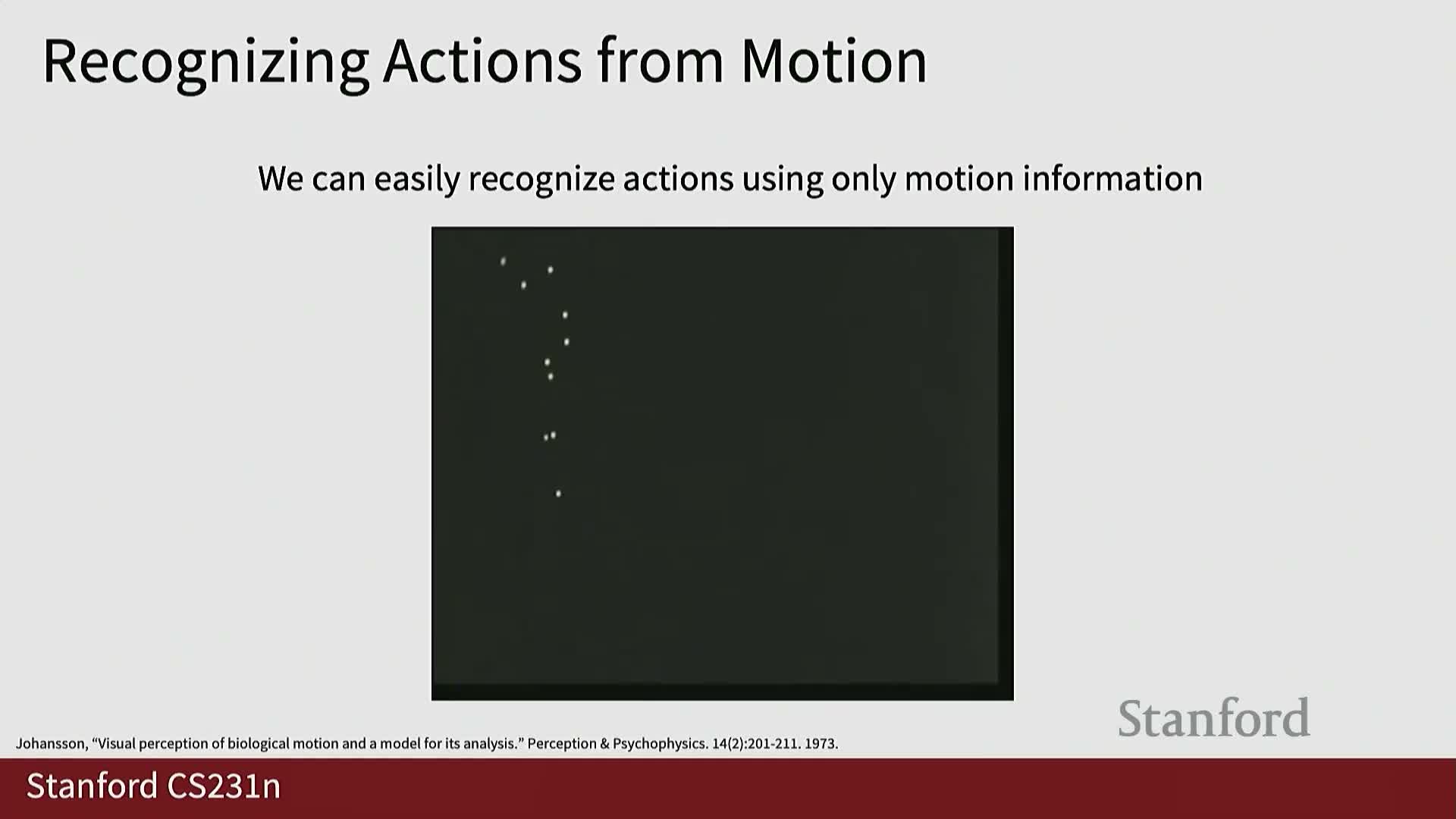
Spatial appearance and temporal motion are fundamentally different signals, motivating explicit motion modeling using optical flow.
Optical flow:
- Estimates per‑pixel 2D motion vectors between adjacent frames.
- Produces horizontal and vertical flow channels that capture low‑level motion cues useful for action recognition and temporal localization.
Two‑stream networks combining appearance and motion streams
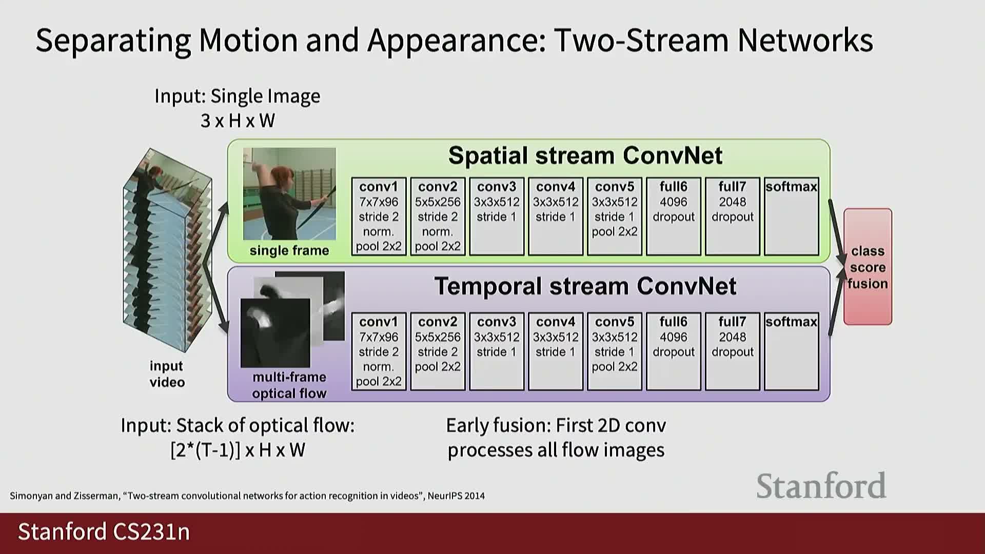
The two‑stream architecture maintains separate networks for RGB appearance and stacked optical‑flow inputs:
- Each stream is trained to predict actions independently.
- Predictions are fused (e.g., score averaging or late fusion) to leverage complementary static and motion information.
Notably, the motion stream often delivers surprisingly strong performance on many action datasets.
Modeling long‑term temporal structure with recurrent models
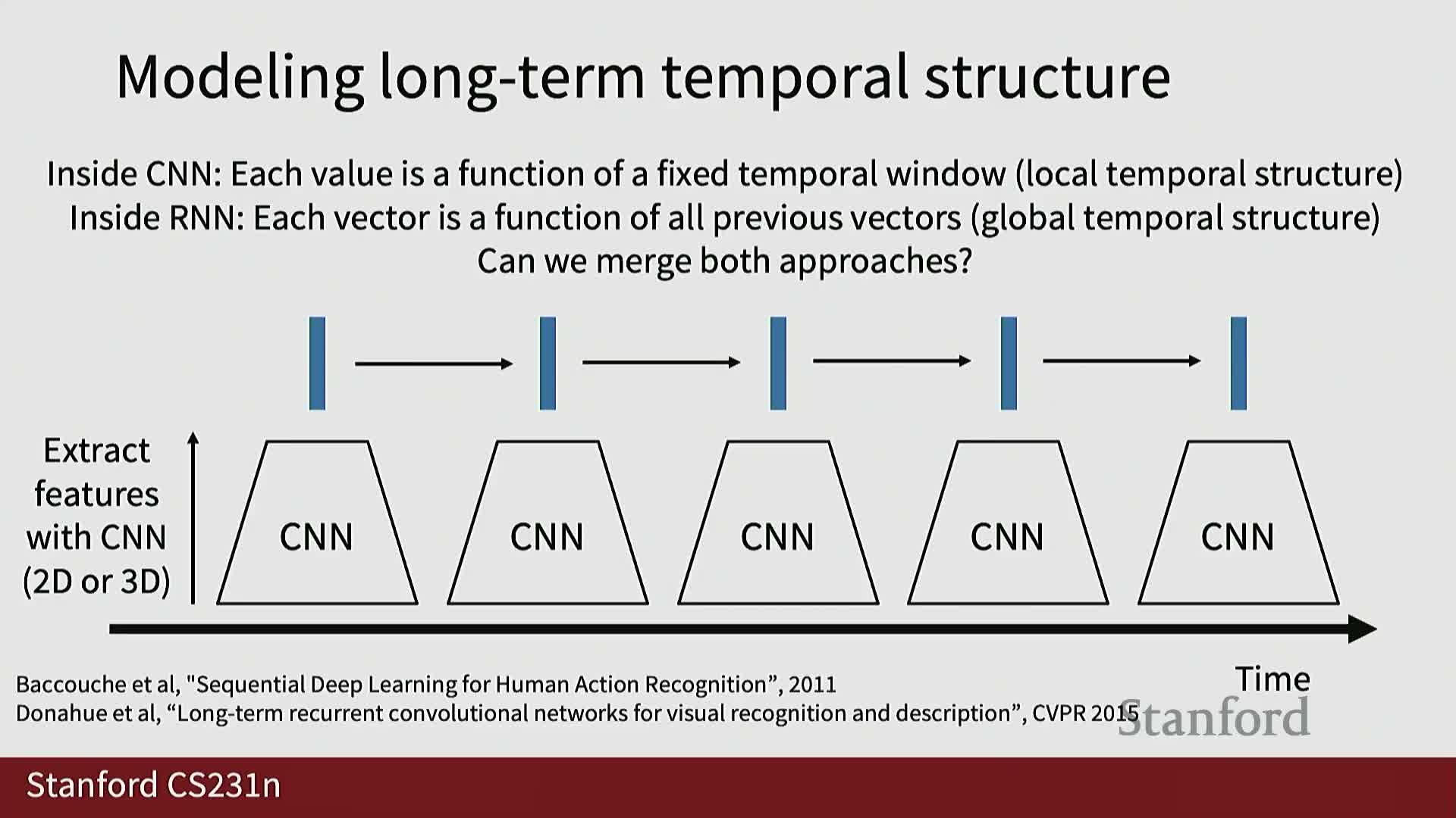
RNNs / LSTMs model longer‑range dependencies by processing sequences of clip‑level or frame‑level features extracted by CNNs:
- They support many‑to‑one mappings (video → label) or sequence outputs (per‑frame predictions).
- Practical considerations include training stability, vanishing gradients, and parallelization limits compared with feedforward alternatives.
Recurrent convolutional networks as spatio‑temporal hybrids
Recurrent convolutional networks (ConvRNNs, ConvLSTM, ConvGRU) replace matrix multiplications inside RNNs with convolutional operations so that hidden states and inputs remain 3D tensors (C×H×W).
This enables spatially localized recurrent updates that naturally fuse temporal recurrence with convolutional spatial modeling—useful when preserving spatial layout across time is important.
Non‑local/self‑attention blocks for spatio‑temporal interaction
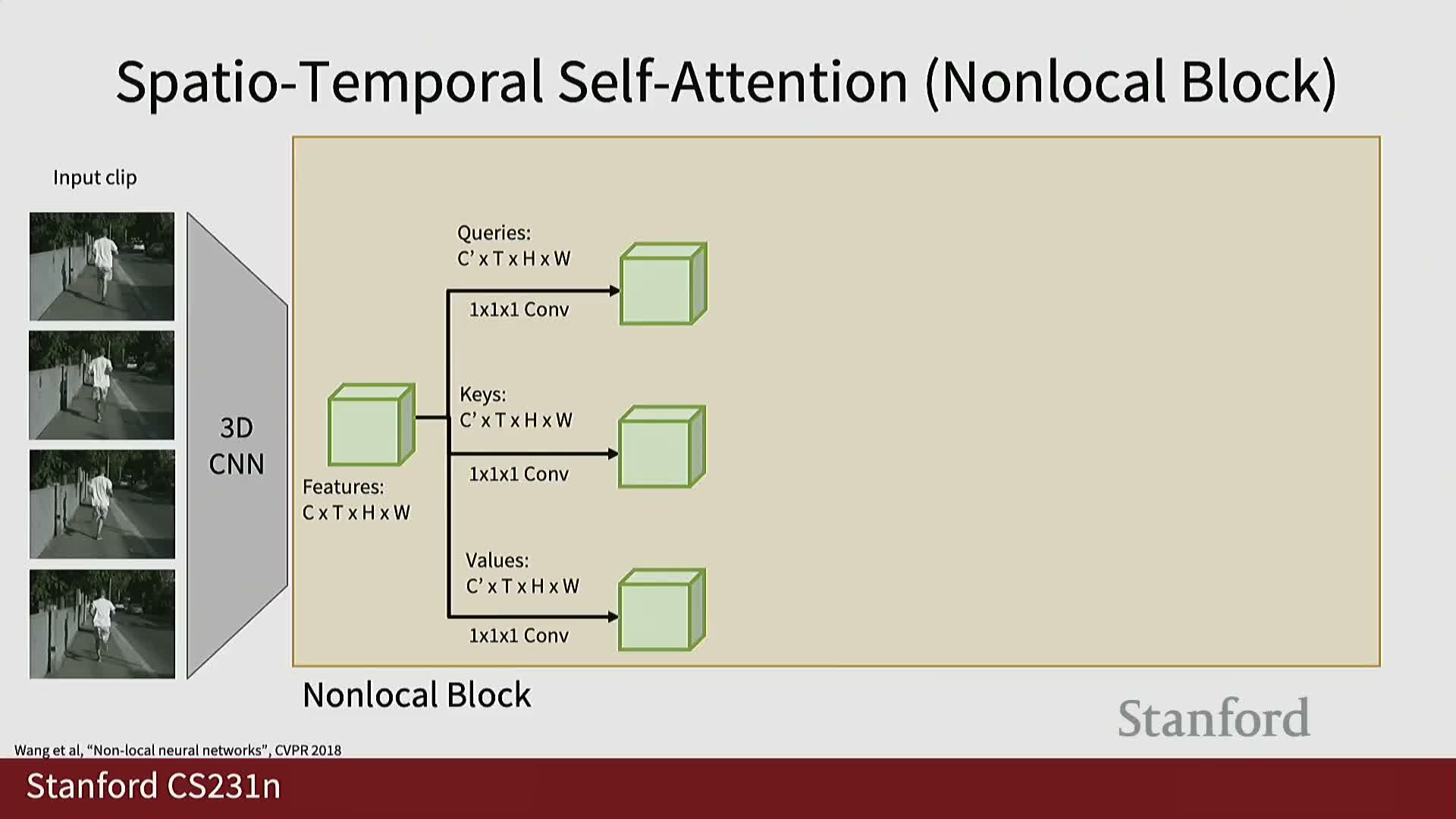
Extending self‑attention to video involves computing query/key/value tensors over C×T×H×W feature maps (often via 1×1×1 convolutions), then forming attention weights between arbitrary spatio‑temporal positions.
Benefits:
- Enables long‑range, highly parallelizable spatio‑temporal interactions.
- Allows the model to directly relate distant spatial locations and time steps without relying solely on local receptive fields.
I3D inflation: transferring 2D architectures and weights to 3D
The I3D approach inflates 2D convolutional kernels into 3D (kT×kH×kW), reusing successful 2D architectures for video.
Practical trick:
- Initialize 3D weights from pretrained 2D weights by copying and scaling along the temporal dimension, giving a strong initialization that improves training stability for video models.
Progress in video architectures and large‑scale performance gains
Recent advances have driven substantial accuracy improvements on large benchmarks (e.g., Kinetics‑400):
-
Factorized space‑time attention, transformer‑based architectures, and MAE‑style pretraining are among the techniques that improved performance.
Contemporary models can achieve much higher top‑1 / top‑5 accuracy compared to earlier baselines when trained at scale.
Visualization via class‑score optimization for appearance and flow streams
Gradient‑based visualization methods for video models optimize input RGB frames or optical‑flow stacks to maximize a target class score:
- Appearance optimizations tend to reveal texture and pose cues.
- Flow optimizations reveal coherent motion patterns that the model finds discriminative for action prediction.
Temporal action localization and spatio‑temporal detection tasks
Temporal action localization is the task of identifying temporal intervals where actions occur; spatio‑temporal detection jointly localizes actions in space and time.
Approaches often adapt object detection techniques to the temporal domain:
- Proposal generation (sliding windows, learned proposals) followed by classification and refinement.
Audio‑visual multimodal tasks and visually‑guided source separation
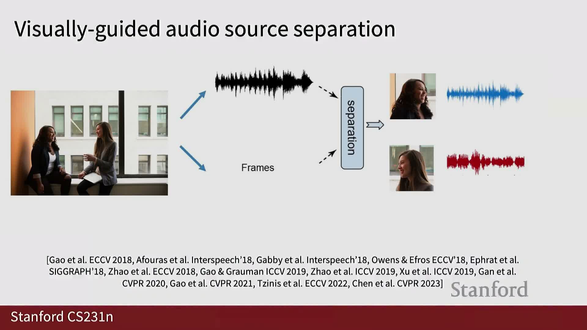
Multimodal video tasks integrate audio and visual streams—for example, visually guided audio source separation, where visual cues (lip motion, instrument movement) help separate mixed audio into constituent sources.
Applications include:
- Speech separation in noisy scenes.
- Musical instrument isolation and enhancement.
Efficiency strategies: clip selection, modality selection and policy learning
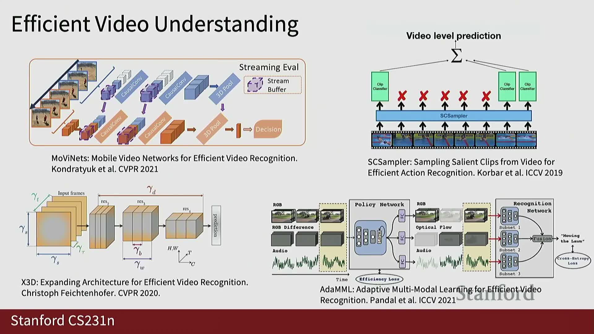
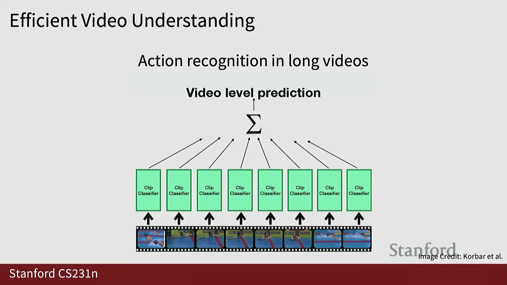
Techniques for efficient video understanding include:
- Compact 3D architectures (e.g., X3D).
-
Learned clip samplers that predict which temporal segments to evaluate.
-
Policy learning methods that adaptively choose modalities or clips to reduce computation while preserving accuracy.
Egocentric multimodal video streams and social interaction understanding
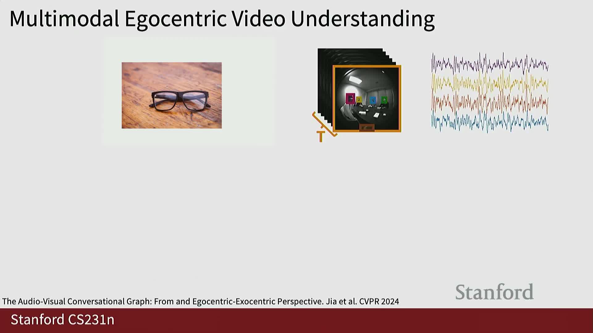
There is growing interest in egocentric (first‑person) multimodal video streams from wearables with multi‑channel audio.
Example tasks:
-
Speaker‑listener identification.
-
Social interaction understanding for real‑time assistance in AR/VR settings.
These tasks exploit spatial, temporal, and audio cues under real‑time constraints.
Connecting video understanding with large language models and video foundation models
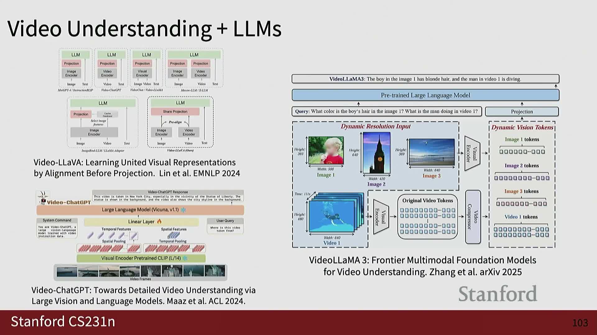
Current efforts aim to build video foundation models that tokenize visual and audio content and map video representations into language model embedding spaces.
Goals:
- Enable promptable video understanding and captioning.
- Leverage pretrained large language models for multimodal reasoning, bridging video representation learning with natural language interfaces.
Enjoy Reading This Article?
Here are some more articles you might like to read next: