Stanford CS231N | Spring 2025 | Lecture 11- Large Scale Distributed Training
- Lecture overview and Llama 3 as a running example
- GPU hardware basics and H100 microarchitecture
- Per-device throughput evolution and impact on AI progress
- Memory and interconnect hierarchy from GPU to full cluster
- Physical constraints, scale metrics and thinking of the data center as one computer
- Alternative training hardware beyond Nvidia GPUs
- Parallelism problem statement and axes for transformer models
- Data parallelism (DP) and synchronized gradient aggregation
- Fully sharded data parallelism (FSDP) to remove per-replica memory bottlenecks
- Hybrid sharded data parallelism (HSDP) and multi-dimensional parallelism
- Activation checkpointing to trade compute for memory
- Scaling recipe and practical thresholds for parallel strategies
- Hardware and model FLOPS utilization (HFU and MFU) as optimization objectives
- Context parallelism, pipeline parallelism, and tensor parallelism
- Integrated multi-dimensional parallelism in production and closing takeaways
Lecture overview and Llama 3 as a running example
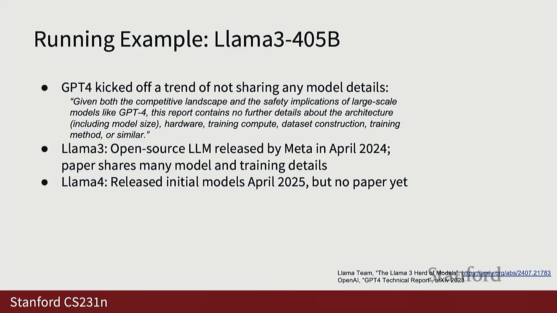
The lecture introduces large-scale distributed training as the dominant paradigm for training modern neural networks and identifies Llama 3 (405B) as a representative, well-documented example for discussing system and algorithmic details.
It situates the shift from single-GPU training a decade ago to current practice where models are routinely trained on tens to tens of thousands of devices, and notes the resulting need for new algorithms and system designs.
The description highlights differences in openness among model providers and why Llama 3 is a useful case study due to the published infrastructure and training details.
The introduction frames the talk into two main parts:
-
Hardware (GPUs and clusters)
-
Distributed training algorithms for exploiting many GPUs
GPU hardware basics and H100 microarchitecture
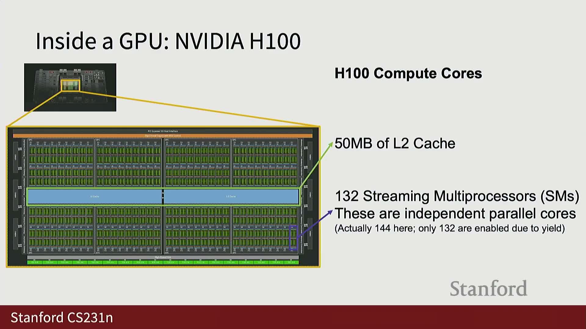
A modern GPU is a general-purpose parallel processor originally designed for graphics workloads and now optimized for high-throughput matrix operations relevant to deep learning.
Key architectural points for the Nvidia H100:
-
HBM (80 GB) is separated from compute cores via a high-bandwidth bus to balance capacity and throughput.
- A multi-level memory hierarchy includes:
-
L2 (≈50 MB) for larger, lower-latency caches
- Per-SM L1/register files (≈256 KB) for very low-latency local state
-
L2 (≈50 MB) for larger, lower-latency caches
- Each H100 contains many streaming multiprocessors (SMs) that host FP32 arithmetic units and specialized tensor cores.
-
Tensor cores execute fixed-size matrix multiply-adds at very high throughput and operate in mixed precision (low-precision inputs with higher-precision accumulation).
Practical note: software that fails to use the supported low-precision formats and mixed-precision execution paths (for example, forgetting to cast tensors to 16-bit) will fall back to slower FP32 units and suffer large slowdowns.
Per-device throughput evolution and impact on AI progress
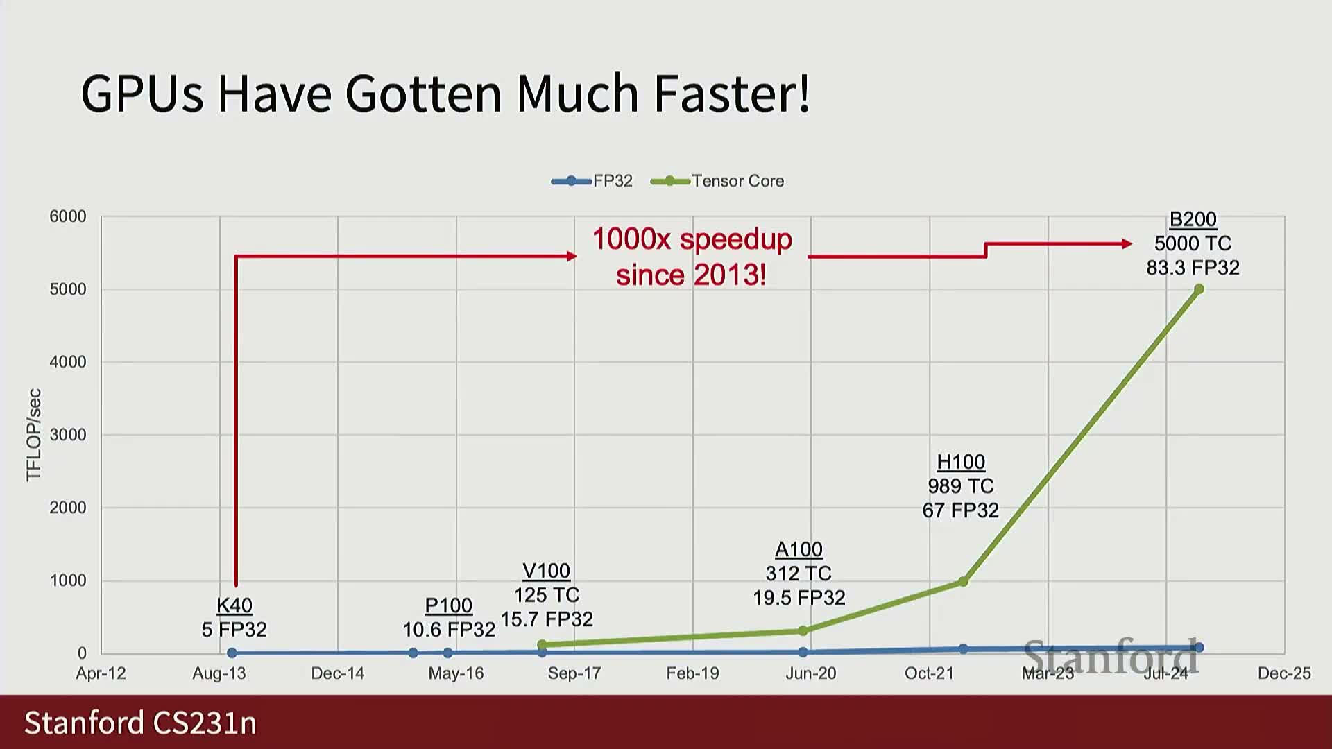
GPU designs that added tensor cores produced a step change in per-device throughput, driving roughly three orders of magnitude improvement in raw FLOPS per device over the past decade.
Highlights and caveats:
- The introduction of tensor cores (for example in the V100) enabled huge increases in mixed-precision matrix throughput relative to earlier FP32-only chips.
- Recent devices advertise enormous theoretical teraflop numbers for both FP32 and mixed-precision tensor-core execution.
- This per-device computational explosion is a major driver behind contemporary advances in deep learning.
- However, theoretical peaks must be tempered by achievable performance in real workloads and by limits in memory and interconnect bandwidth.
Memory and interconnect hierarchy from GPU to full cluster
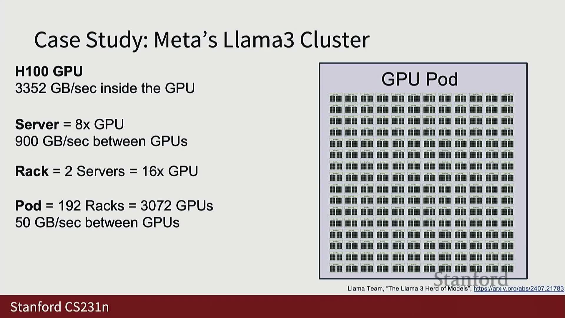
Compute performance must be considered in the context of a multi-scale memory and interconnect hierarchy that extends from on-die caches and HBM to intra-server PCIe/NVLink and inter-rack links.
Bandwidth examples and implications:
- A single GPU can move data from its HBM at multiple terabytes per second.
-
Intra-server GPU-to-GPU links typically provide hundreds of GB/s.
-
Cross-rack or pod-level connectivity can drop to tens of GB/s or less.
- These bandwidth drops require algorithms that minimize cross-node traffic or hide communication behind computation.
Concrete Llama 3 training-cluster example:
- GPUs are packaged in servers (8 GPUs per server).
- Servers are grouped in racks.
- Racks form pods (e.g., 192 racks → ≈3072 GPUs with ≈50 GB/s pairwise within-pod bandwidth).
- Pods are combined into clusters (e.g., 8 pods → 24,576 GPUs) with yet lower bandwidth between pods.
Physical constraints, scale metrics and thinking of the data center as one computer
Large training clusters occupy substantial physical space and power, require extensive cooling and networking infrastructure, and are naturally organized into racks and pods because of data center constraints.
Important operational points:
- Aggregating many GPUs into one logical computer enables treating the entire facility as a single supercomputer with aggregated memory capacity, core counts, and exascale-class FLOPS.
- This abstraction requires careful handling of the hierarchical communication costs introduced by the physical layout.
- Typical long training runs last months, so system design trade-offs (physical layout, cooling, storage racks, and networking hardware) materially affect what parallelization patterns and scales are practical.
Alternative training hardware beyond Nvidia GPUs
Although Nvidia GPUs (H100 series) are currently dominant for large-scale training, other architectures exist and present alternative trade-offs:
-
Google TPUs (e.g., V5P): Google-designed matrix-acceleration devices available via Google Cloud or internally. They provide comparable mixed-precision throughput and use a pod-based scalability model, but differ in microarchitectural choices and availability constraints.
-
AMD MI-series and other vendor accelerators: offer competitive peak metrics but differ in software ecosystem maturity, interconnect designs, and market adoption.
-
Cloud vendor chips (AWS, proprietary silicon): provide alternative trade-offs in availability, integration, and ecosystem support.
Practical point: peak FLOPS are only one axis—software ecosystem, interconnect, and adoption determine practical accessibility and overall impact for large-scale training.
Parallelism problem statement and axes for transformer models
Training on thousands of devices requires splitting computation across multiple axes to expose massive parallelism while respecting the memory and communication hierarchy.
For transformer models the computation naturally sits in a 3D tensor (batch × sequence × hidden-dimension) stacked across L layers, yielding common parallelization axes:
-
Data (batch) parallelism
-
Context (sequence) parallelism
-
Tensor (model-dimension) parallelism
-
Layer- or pipeline-parallelism (including pipeline-style layer partitioning)
Designing a distributed training strategy is therefore a problem of:
- Choosing how to partition these axes.
- Scheduling communication to match hardware topology.
- Overlapping communication with computation to maximize useful work across devices.
Data parallelism (DP) and synchronized gradient aggregation
Data parallelism (DP) replicates model weights across multiple devices, assigns different mini-batch shards to each replica, computes local forward and backward passes independently, and then performs an all-reduce to aggregate gradients before applying synchronized weight updates.
Process (high-level):
- Replicate weights on each device.
- Assign a distinct mini-batch shard to each replica and run local forward/backward.
- Use an all-reduce to sum/average gradients across replicas.
- Apply a synchronized weight update so each replica keeps identical weights.
Notes and best practices:
- Mathematically exact because gradients are linear and per-sample gradient averages commute with summation across devices.
- Effective DP implementations overlap local backward computation with gradient communication (for example, by pipelining layer-wise reductions) to hide communication latency.
- Frameworks such as PyTorch DistributedDataParallel provide common, optimized implementations.
-
Asynchronous SGD variants exist but tend to be less stable and harder to reproduce.
Fully sharded data parallelism (FSDP) to remove per-replica memory bottlenecks
Fully Sharded Data Parallelism (FSDP) eliminates the per-replica model-copy memory bottleneck by partitioning model parameters and optimizer state across devices so each parameter has a unique owner device.
High-level flow:
- During the forward pass owners broadcast parameter shards to participants as needed.
- Participants compute activations and then drop the parameter copy to save memory.
- During backward, the owner gathers local gradients for its owned shard and computes global updates locally.
- Owners maintain optimizer state and perform local updates.
Trade-offs:
-
FSDP reduces memory duplication and enables training much larger models than naive DP.
- It introduces repeated weight broadcasts and gradient gathers per layer, increasing communication complexity.
- Careful overlap of communication with computation is required to avoid throughput regressions.
Hybrid sharded data parallelism (HSDP) and multi-dimensional parallelism
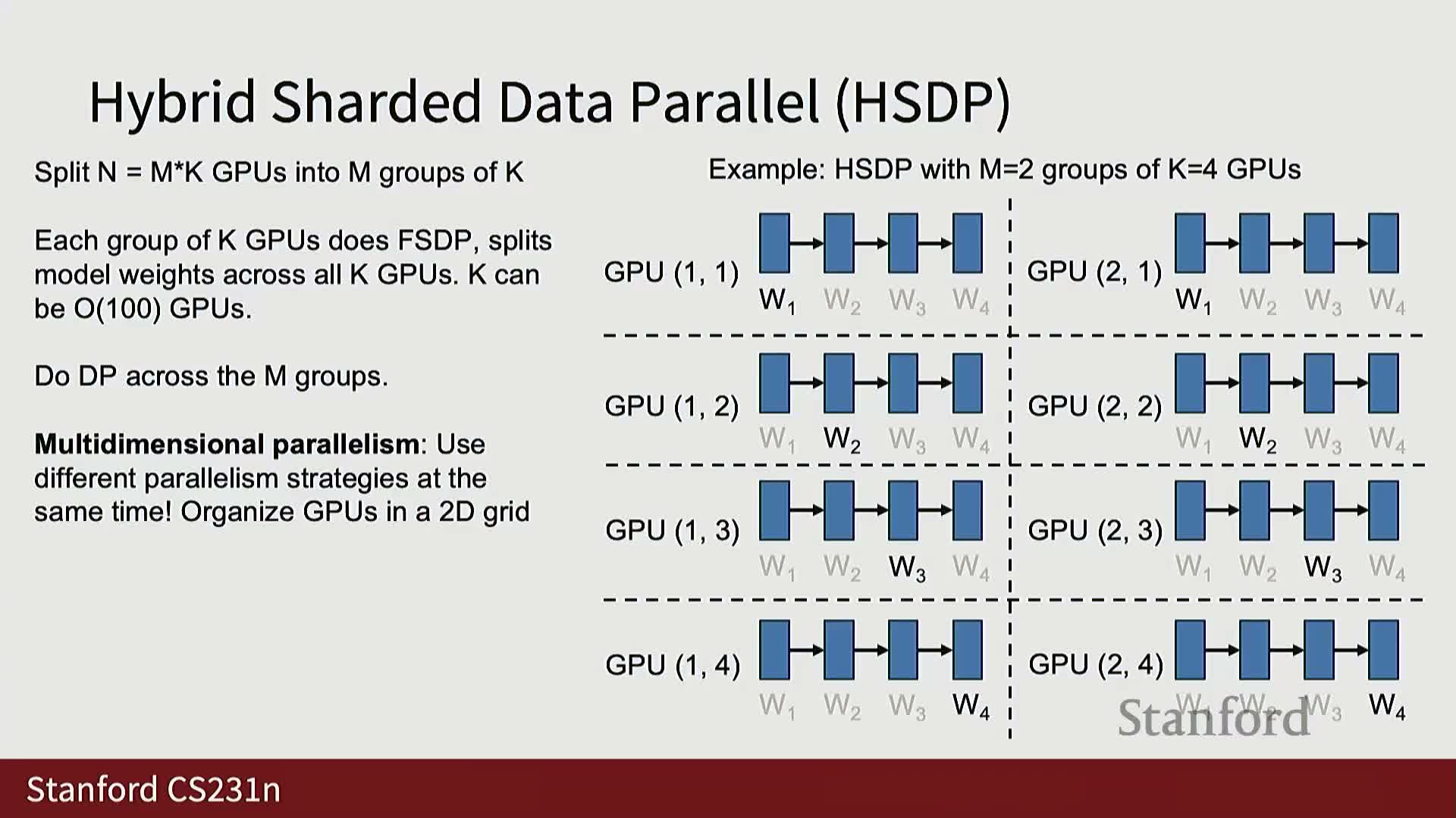
Hybrid Sharded Data Parallelism (HSDP) arranges devices in a two-dimensional grid combining fully sharded groups along one axis and replicated data-parallel groups along the other, enabling a trade-off between memory savings and reduced cross-group communication.
Concretely:
- Form K-device groups that perform FSDP internally to shard weights and reduce intra-group memory.
- Form M replicated groups that then perform inter-group all-reduces to obtain macro-batch gradients.
- This split maps well to hierarchical hardware topologies where intra-server connectivity is faster than cross-server links.
Practical benefit: HSDP reduces the amount of weight broadcast traffic across slow links and leverages faster local connectivity for the heavier FSDP operations, making it useful when scaling beyond a few hundred GPUs.
Activation checkpointing to trade compute for memory
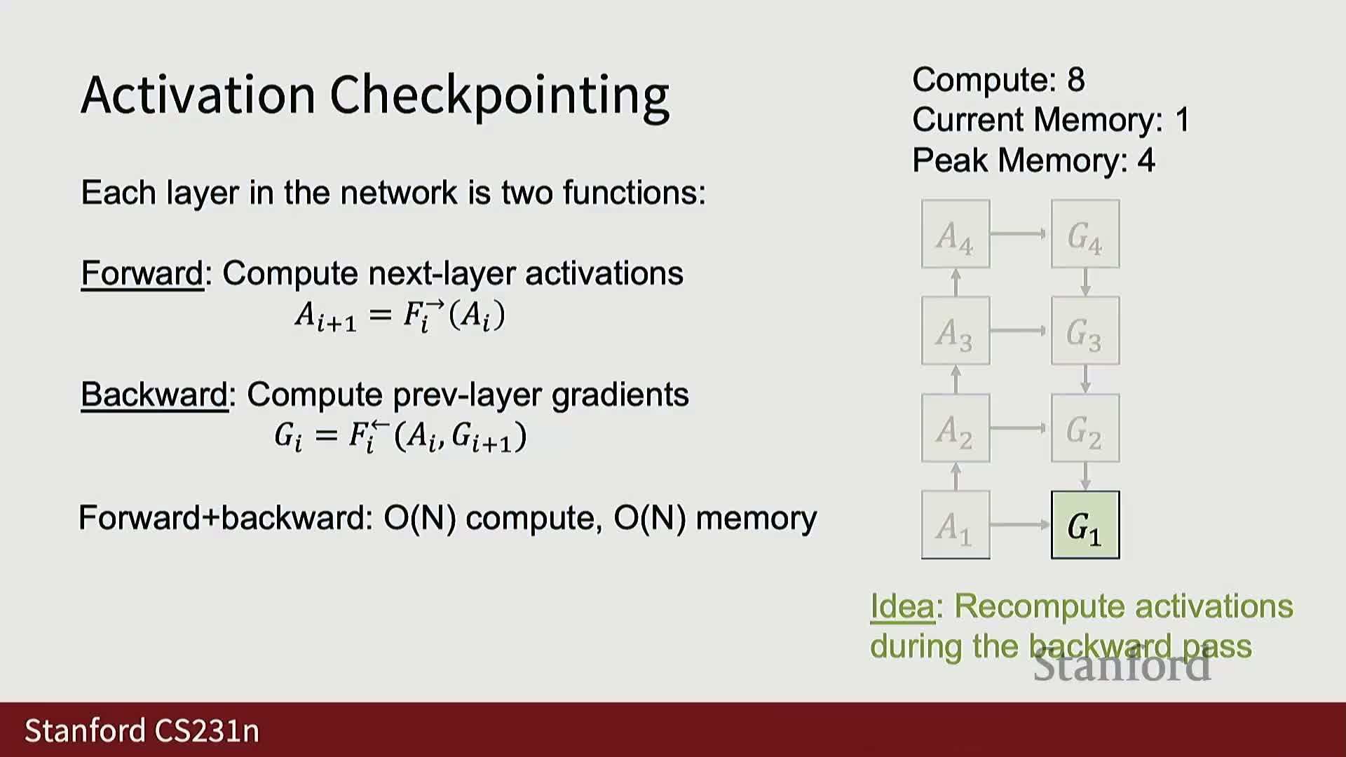
Activation checkpointing reduces peak activation memory by discarding intermediate activations during the forward pass and recomputing them during the backward pass, trading increased compute for a lower memory footprint.
Cost/benefit and complexity:
- A naive recomputation strategy that re-evaluates every layer gives O(n^2) extra compute for an n-layer network with constant memory.
- Checkpointing at intervals of C layers yields roughly O(n^2 / C) extra compute and O(C) memory.
- A common practical choice is C ≈ √n, which gives approximately O(n√n) compute and O(√n) memory.
Practical note: checkpointing is essential when activations dominate memory for very deep or wide models, enabling larger sequence lengths or model sizes at the cost of increased wall-clock computation and careful scheduling.
Scaling recipe and practical thresholds for parallel strategies
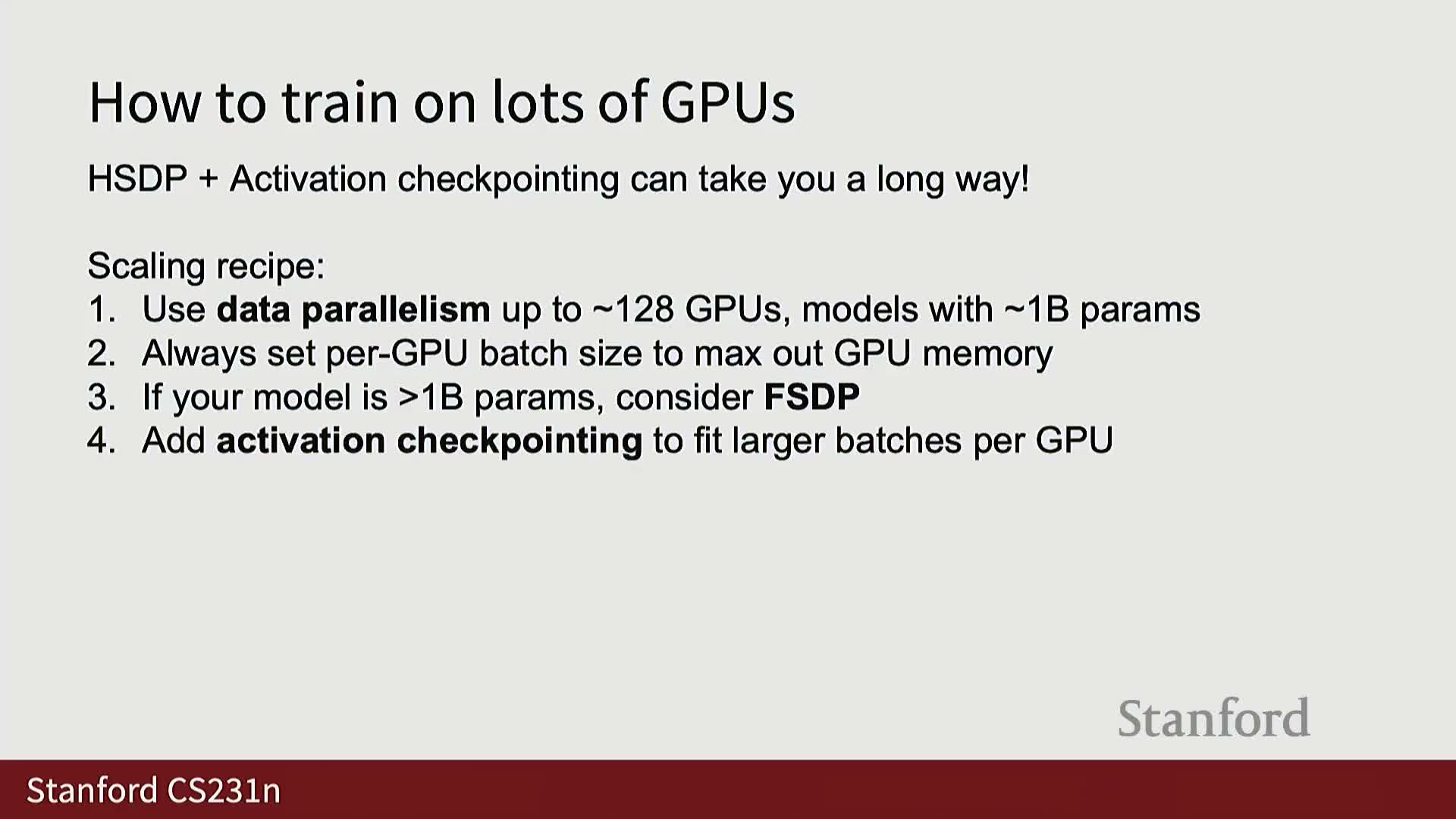
A practical scaling recipe sequences parallel strategies by problem scale and resource availability:
- Use simple data parallelism up to roughly O(128) GPUs and about ~1B parameters.
- Switch to FSDP when model parameters exceed per-device memory.
- Enable activation checkpointing when activations begin to dominate GPU memory.
- Adopt hybrid sharding (HSDP) as group sizes grow to several hundred devices.
- For extremely large models, further partition via tensor parallelism, pipeline parallelism, and context (sequence) parallelism.
These staged transitions balance memory, communication, and computation to maximize throughput as model and cluster scales grow. Exact thresholds depend on GPU memory capacity, interconnect bandwidth, sequence length, and desired global batch size.
Hardware and model FLOPS utilization (HFU and MFU) as optimization objectives
Two practical utilization metrics to guide tuning:
-
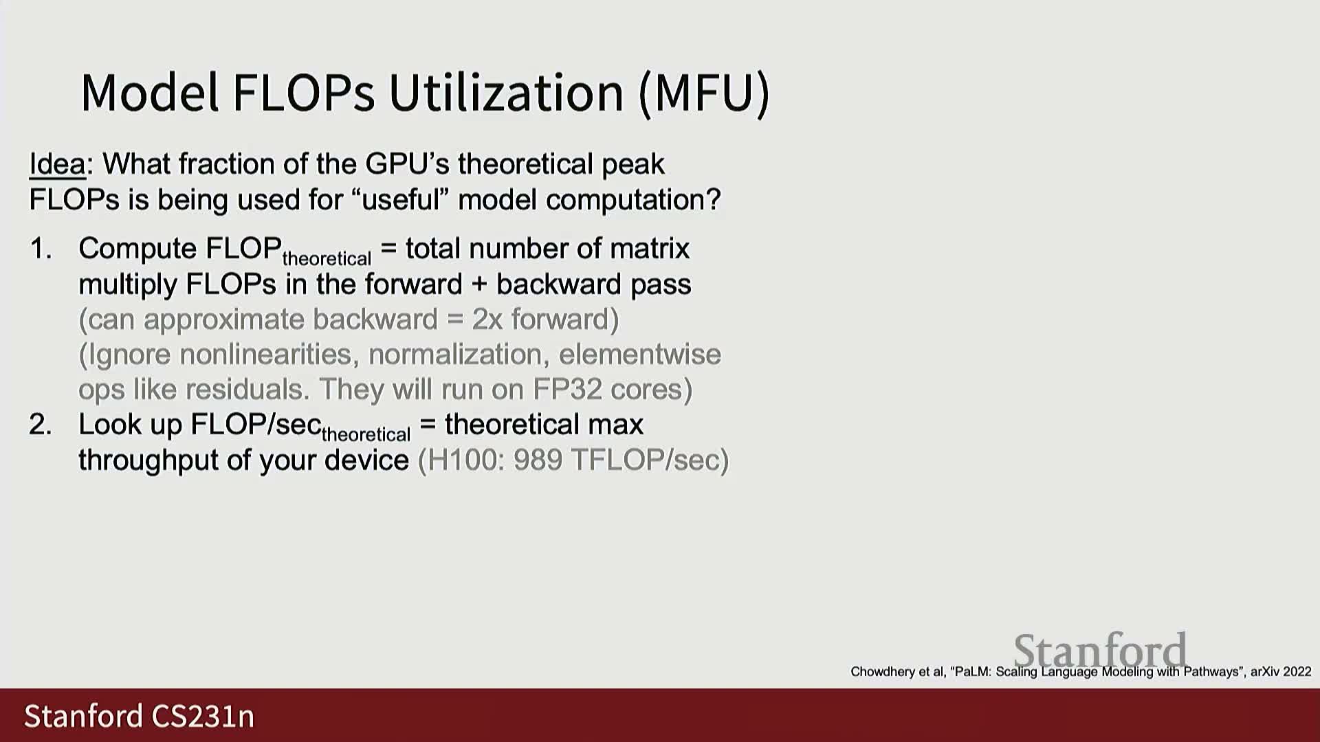
Hardware FLOPS Utilization (HFU): the fraction of a device’s theoretical peak FLOPS actually achieved by low-level kernels.
-
Model FLOPS Utilization (MFU): the fraction of device peak FLOPS spent computing the model’s forward/backward rather than doing IO, communication, or recomputation.
MFU is computed as:
- MFU = (model’s theoretical FLOP count per iteration) / (device peak FLOPS × measured iteration time)
Practical guidance:
-
MFU is the primary metric to guide tuning across batch size, parallelism dimensions, checkpointing, and micro-batching.
- Typical good MFU targets for modern training are > ~30%; excellent designs reach ~40% or higher.
- Published large-scale runs (e.g., Llama 3) report MFUs in the high-30s to low-40s on large GPU fleets, reflecting interconnect and system overheads.
Context parallelism, pipeline parallelism, and tensor parallelism
Parallelism axes and their practical implications:
-
Context (sequence) parallelism partitions long input sequences across devices so each device processes a subsequence. It is attractive when sequence length is the limiting axis but complicates attention (all-pairs interactions) and requires special attention algorithms or head-parallel variants.
-
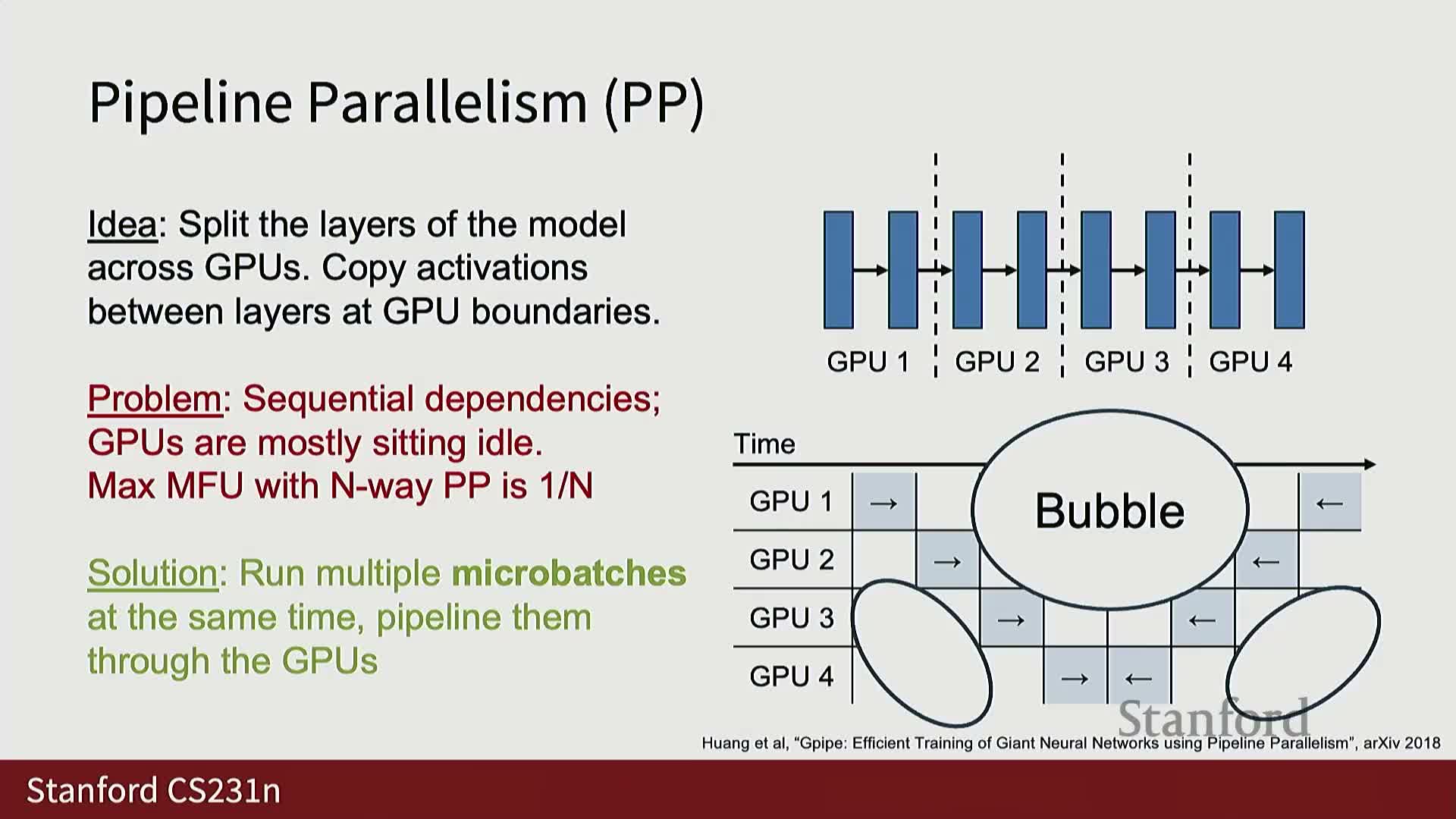
Pipeline parallelism partitions layers across devices and amortizes the pipeline “bubble” by running multiple microbatches concurrently so devices stay busy. This increases activation memory pressure and typically requires checkpointing and micro-batch tuning to maximize utilization.
-
Tensor parallelism partitions large weight matrices across devices and computes block-matrix multiplies in parallel. Clever blocking and pairing of consecutive layers can reduce intermediate communication—for example, two-layer MLP structures in transformers are amenable to efficient tensor-parallel splits.
In practice, modern training pipelines combine these axes (N-D parallelism) with topology-aware placement to exploit intra-node high-bandwidth links and minimize slow cross-pod traffic.
Integrated multi-dimensional parallelism in production and closing takeaways
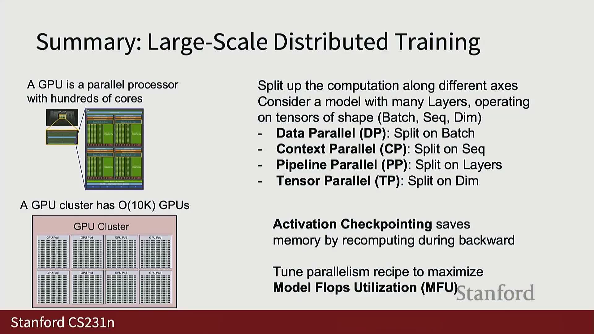
State-of-the-art large-scale training uses all axes of parallelism together: for example, production Llama 3 training mixes tensor, context, pipeline, and data parallelism across thousands of GPUs to balance memory and communication at each hierarchical level.
Engineering goals and practical takeaways:
- Treat the entire cluster as one giant parallel computer while designing algorithms that partition computation, overlap communication with compute, and maximize model FLOPS utilization.
- Understand device and cluster memory hierarchies.
- Apply staged parallel strategies as model and sequence scales grow.
- Use activation checkpointing when necessary.
- Optimize for MFU as the single guiding performance metric.
Enjoy Reading This Article?
Here are some more articles you might like to read next: