Stanford CS231N Deep Learning for Computer Vision | Spring 2025 | Lecture 13- Generative Models 1
- Recap of self-supervised learning and pretext-task two-stage training
- Contrastive learning pulls augmentations of the same sample together and pushes different samples apart
- SimCLR requires large batch sizes to provide sufficient negative examples for effective contrastive learning
- Momentum Contrast (MoCo) provides large pools of negatives using a momentum-updated encoder and a queue
- DINO and DINOv2 apply momentum encoders and modified losses to scale self-supervised training to very large datasets
- Generative models are the main topic and have progressed dramatically with scale and training recipes
- Supervised versus unsupervised learning: objectives and outcomes
- Discriminative models learn conditional distributions P(Y|X) and lack a notion of global data probability
- Generative models learn P(X) or P(X|Y) and induce a global competition for probability mass among inputs
- Practical uses: discriminative models for prediction and features; conditional generative models for controllable sampling
- Taxonomy of generative modeling approaches: explicit vs implicit and direct vs indirect sampling
- Explicit density autoregressive models train by maximum likelihood using the chain rule factorization
- Autoregressive modeling and maximum likelihood estimation (MLE) reduce joint density learning to sequential conditional prediction
- Autoencoders use a bottleneck to learn compressed representations; variational autoencoders add a probabilistic latent prior to enable sampling
- VAE probabilistic formulation uses a decoder p_theta(X|Z) and an encoder q_phi(Z|X) that outputs parametric Gaussian distributions
- The evidence lower bound (ELBO) provides a tractable training objective that trades exact likelihood for a computable lower bound
- VAE training uses the reparameterization trick, balances reconstruction and prior terms, and enables latent interpolation and sampling
Recap of self-supervised learning and pretext-task two-stage training
Self-supervised learning trains an encoder–decoder system on large unlabeled datasets by defining a pretext task that produces supervisory signals from the data itself.
The approach typically follows a two-stage procedure:
- Train an encoder and decoder jointly on the pretext objective using massive unlabeled image collections.
- Discard the decoder and reuse the encoder features (optionally with a small classifier head) on downstream labeled tasks.
Common pretext tasks force the encoder to learn structure and invariances in natural images:
-
Rotation prediction — predict image rotation angle.
-
Patch rearrangement (jigsaw) — predict correct patch ordering.
-
Reconstruction / inpainting — reconstruct missing or corrupted regions.
Key operational points:
- The method leverages scale — millions to billions of unlabeled samples — to produce transferable representations for problems with limited labeled data.
- Important implementation choices include augmentation policy, encoder architecture, and whether to fine-tune the encoder end-to-end on downstream tasks.
Contrastive learning pulls augmentations of the same sample together and pushes different samples apart
Contrastive learning builds representations by forming multiple views (augmentations) per input and training a feature extractor so that:
- Representations of augmentations from the same image are similar (positive pairs).
- Representations from different images are dissimilar (negatives).
Typical training pipeline:
- Apply random augmentations to each image to form positive pairs.
- Pass all augmented views into a neural feature extractor.
- Compute pairwise similarities across the minibatch to implement a contrastive objective (often using a large similarity matrix).
Practical considerations:
- Losses encourage high similarity for positives while treating other views as negatives.
- The approach relies heavily on effective augmentations and having enough distinct negatives per optimization step for a strong learning signal.
- Common encoders: CNNs or Vision Transformers; tune augmentation policies and temperature hyperparameters for best performance.
SimCLR requires large batch sizes to provide sufficient negative examples for effective contrastive learning
SimCLR-style contrastive methods compute similarities among all augmented views in a minibatch and designate the two augmentations of the same image as positives, treating all other views as negatives.
Consequences and tradeoffs:
- The number of negatives is proportional to batch size.
- With small batches the task becomes too easy (too few negatives), degrading feature learning.
- State-of-the-art representations typically require very large minibatches or distributed training.
Design responses to this dependence:
- Decouple the number of available negatives from instantaneous minibatch size (e.g., memory banks).
- Cache negatives from previous iterations (queues).
- Practitioners balance batch size, augmentation strength, and temperature to obtain good convergence.
Momentum Contrast (MoCo) provides large pools of negatives using a momentum-updated encoder and a queue
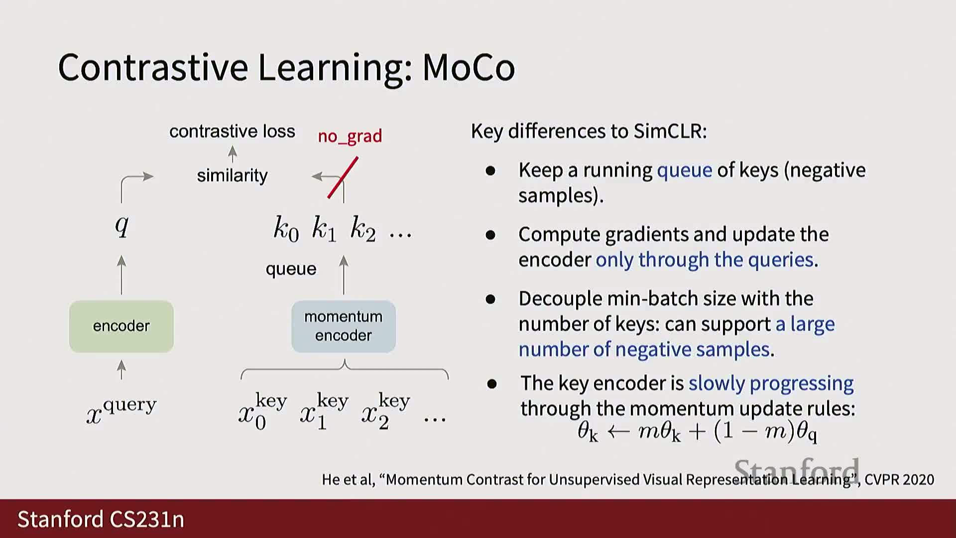
MoCo builds a dynamic dictionary of negative keys by maintaining a queue of feature representations from previous minibatches and using a separate momentum encoder to compute keys for those stored negatives.
How it works:
- The primary encoder is updated via gradient descent on the current minibatch.
- The momentum encoder (used to encode keys placed into the queue) is updated as an exponential moving average of the primary encoder weights, e.g. new_m = m_old * 0.99 + primary * 0.01, which:
- avoids backpropagating through the large queue, and
- stabilizes the key representations.
- At each iteration the current minibatch features act as queries and the queue supplies many negatives, enabling effective contrastive training without extremely large instantaneous batch sizes.
Practical benefits:
- Reduces memory pressure.
- Enables large effective negative sets while keeping per-step batch sizes reasonable.
- Has influenced many follow-up self-supervised architectures.
DINO and DINOv2 apply momentum encoders and modified losses to scale self-supervised training to very large datasets
DINO (and DINOv2) uses a dual-encoder approach similar to MoCo with a momentum encoder, but replaces some loss choices and introduces stabilization mechanisms.
Key algorithmic and recipe changes:
- Replace simple softmax cross-entropy with alternatives such as KL-divergence-based objectives and centering mechanisms.
- Careful normalization/centering and tailored augmentation schemes improve stability and representation quality.
Empirical scaling:
-
DINOv2 shows that with careful recipes this architecture can scale beyond ImageNet to tens or hundreds of millions of images (e.g., ~142 million images), producing robust self-supervised features that transfer well to downstream tasks.
Practical outcome:
- Contributions are both algorithmic (loss variants, normalization, augmentations) and empirical (large-scale data and compute).
- Resulting pretrained models are commonly used for feature extraction and fine-tuning in practical workflows.
Generative models are the main topic and have progressed dramatically with scale and training recipes
Generative modeling treats generation as probabilistic modeling of high-dimensional data and has progressed from blurry outputs to realistic image, video, and language generation through algorithmic innovations, larger datasets, more compute, and stable training recipes.
High-level taxonomy and concerns:
- Models either explicitly model densities or implicitly provide sampling mechanisms.
- Some methods give direct, fast sampling; others require iterative procedures.
- Modern generative models underpin language models and conditional image synthesis systems and require careful handling of probabilistic objectives, architectures, and sampling procedures to scale.
The subsequent discussion contrasts generative objectives and situates modern methods within a taxonomy of explicit/implicit and direct/iterative approaches.
Supervised versus unsupervised learning: objectives and outcomes
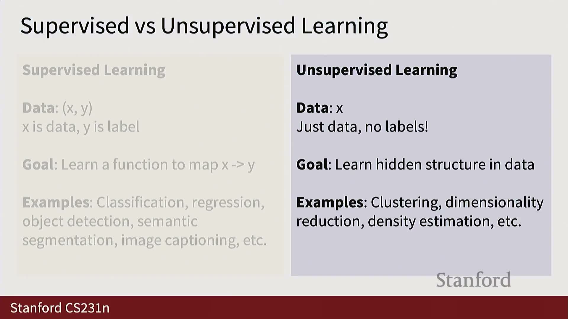
Supervised learning trains models to map inputs X to labels Y using paired examples (X,Y), optimizing a loss that encourages correct label prediction and generalization to new inputs.
Examples and contrasts:
- Classic supervised tasks: classification, detection, segmentation.
-
Unsupervised learning (including self-supervised learning) operates on unlabeled data X to uncover structure, representations, or density estimates without a specific prediction target. Examples include k-means (clustering), PCA (dimensionality reduction), and density estimation.
Operational distinction:
-
Supervised models learn conditional distributions **P(Y X)** and are tailored to a specific task.
- Unsupervised models aim for general-purpose structure or factors of variation that can transfer to tasks with limited labels.
- Modern pipelines often combine both paradigms: learn unsupervised representations at scale, then fine-tune them for downstream supervised tasks.
Discriminative models learn conditional distributions P(Y|X) and lack a notion of global data probability
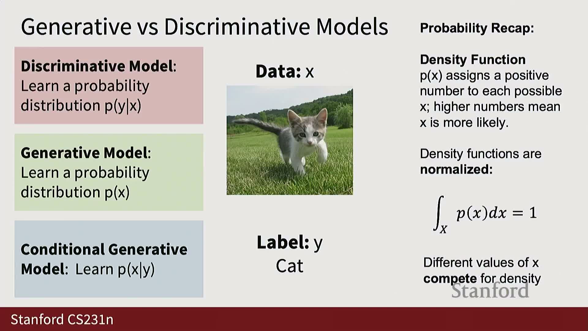
Discriminative probabilistic models focus on modeling the distribution of labels or targets Y conditioned on a given input X, i.e., they model P(Y|X).
Key properties:
- For each X the model produces a normalized distribution over labels; normalization occurs over labels, not over inputs.
- Because normalization is per-input, there is no competition among different inputs for probability mass — the model cannot naturally reject out-of-distribution (OOD) inputs and must assign probabilities across the fixed label set.
- Discriminative models are appropriate when the task is prediction of Y from X or when learning features useful for downstream tasks.
- They are typically trained with cross-entropy or equivalent objectives that maximize conditional log-likelihood across training pairs.
Practical limitation:
- The inability to represent global outlier likelihoods hinders OOD detection when needed.
Generative models learn P(X) or P(X|Y) and induce a global competition for probability mass among inputs
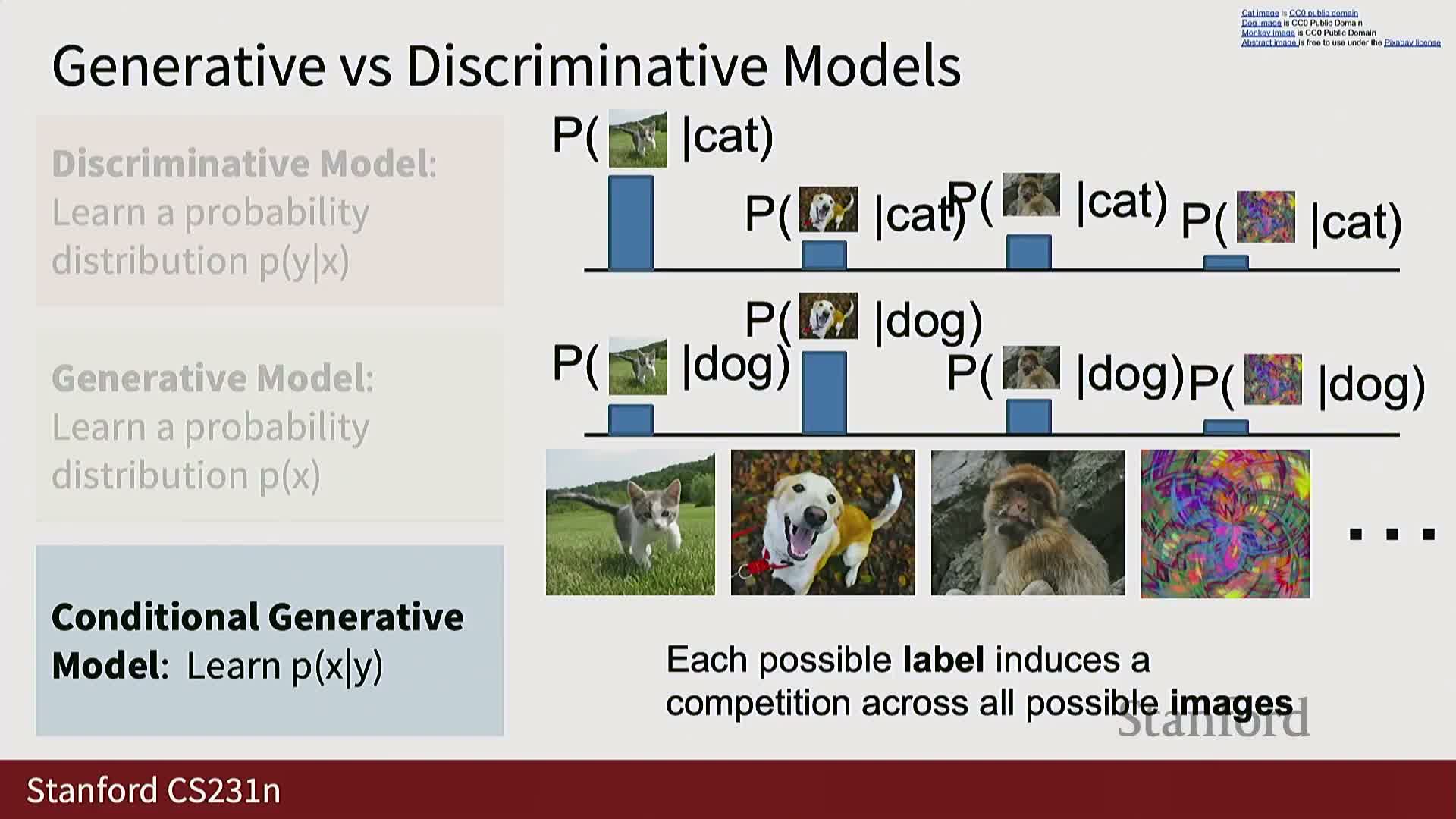
An unconditional generative model specifies a probability distribution P(X) over all possible data instances X so that all candidate images compete for finite probability mass; modeling P(X) therefore requires capturing which images are typical and which are unlikely under the data-generating process.
In contrast, a conditional generative model P(X|Y) defines, for each conditioning value Y, a distribution over images, enabling:
-
Controlled synthesis (sample conditioned on labels, text, or other modalities).
- The ability to assign low probability to inputs outside the conditional support.
Consequences of global normalization:
- Forces the model to internalize rich structural assumptions about the data manifold and to reason about which variants are more likely.
- Enables outlier detection, principled sampling, and composition with discriminative components via Bayes’ theorem, but increases modeling complexity compared to discriminative formulations.
Practical uses: discriminative models for prediction and features; conditional generative models for controllable sampling
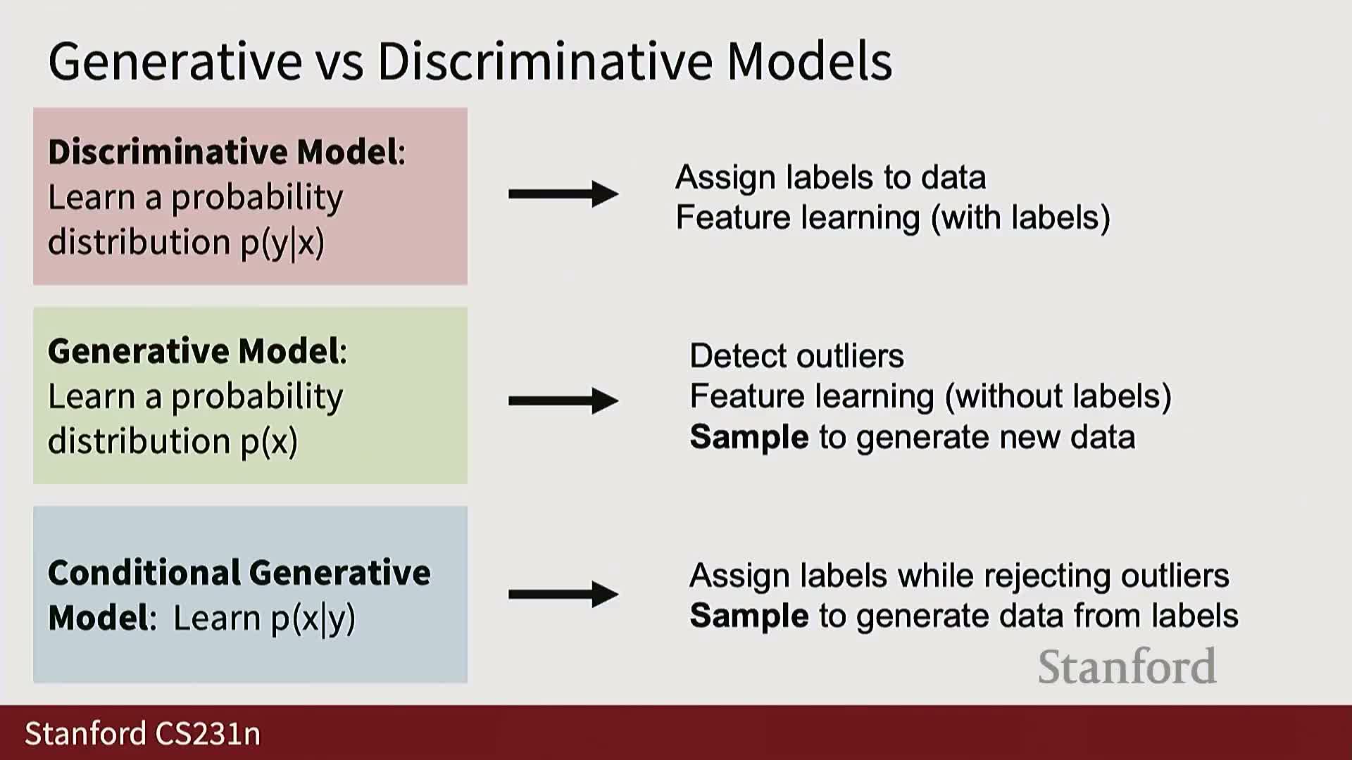
Use cases and practical trade-offs across model types:
-
Discriminative models — primarily used for direct prediction tasks and for learning transferable representations.
-
Unconditional generative models — mainly useful for density estimation and outlier detection, but offer limited control for synthesis.
-
Conditional generative models — most practically valuable because they provide controllable sampling conditioned on labels, text, or other modalities (e.g., text-to-image, conditional video prediction).
Practical training note:
- Although Bayes’ rule relates discriminative and generative models theoretically, composing separate components is often impractical.
-
In practice, conditional generative models are usually trained directly and end-to-end rather than composing P(Y X) and P(X).
Taxonomy of generative modeling approaches: explicit vs implicit and direct vs indirect sampling
Generative methods split along whether they provide an explicit tractable density P(X) or only allow sampling without accessible density values (implicit density methods).
Explicit density models:
- Enable direct likelihood evaluation and maximum likelihood training.
- Include exact methods (e.g., autoregressive models that factor the joint via the chain rule) and approximate methods (e.g., variational autoencoders (VAEs) that optimize a lower bound on likelihood).
Implicit density models:
- Focus on sample generation without providing tractable likelihoods.
- Some are direct implicit methods that produce samples with a single forward pass (e.g., GAN generators).
- Others are indirect implicit methods that require iterative procedures to sample (e.g., diffusion models, MCMC).
Choice considerations:
- Select a family based on whether likelihood evaluation, sampling speed, or constrained latent structure is the primary requirement.
Explicit density autoregressive models train by maximum likelihood using the chain rule factorization
Autoregressive models decompose the joint density P(X) into a product of conditional distributions across a canonical ordering of the data: P(X) = ∏t P(X_t | X{<t}).
Implications and implementation:
- Convert high-dimensional density estimation into a sequence of conditional prediction problems.
-
Maximum likelihood training reduces to fitting a model that predicts each next element given the prefix; the log-likelihood decomposes into a sum of per-step log-probabilities.
- Architectures that naturally implement this pattern include recurrent neural networks (RNNs) and causal (masked) transformers, which maintain a hidden summary of the prefix and output a distribution for the next token.
- Particularly well-suited to language (discrete 1D sequences).
- Direct pixel-level autoregressive modeling of images requires extremely long sequences and is computationally expensive; tokenization or higher-level sequence representations mitigate this cost in practical image autoregressive models.
Autoregressive modeling and maximum likelihood estimation (MLE) reduce joint density learning to sequential conditional prediction
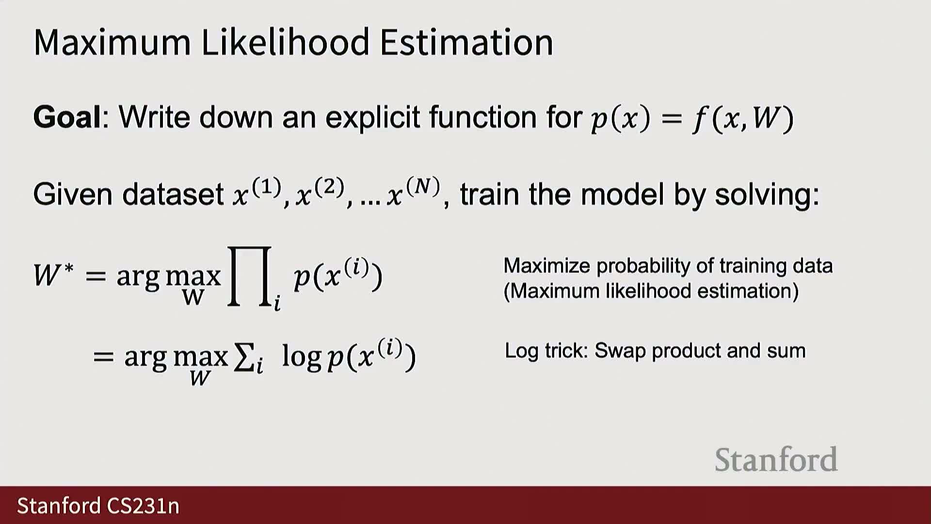
Maximum likelihood estimation (MLE) fits a parameterized density to observed samples by maximizing the product (or sum of log-probabilities) of the model’s probabilities on training points under the iid assumption.
Operational details:
- For autoregressive models the chain rule factors the joint into per-step conditionals, so the log-likelihood decomposes into a sum of per-step log-probabilities.
- This yields a sequence prediction loss implemented via cross-entropy for discrete data.
- Architectures such as RNNs or masked transformers map the prefix to a distribution over the next element; at evaluation the full joint is recovered by multiplying per-step conditionals (or summing log-probabilities).
- MLE trades modeling a combinatorially large joint distribution for modeling many simpler conditional distributions that share parameters.
Autoencoders use a bottleneck to learn compressed representations; variational autoencoders add a probabilistic latent prior to enable sampling
A classical autoencoder is a deterministic encoder–decoder pair that compresses input X into a lower-dimensional latent code Z and reconstructs X from Z; the bottleneck forces the encoder to capture essential structure.
To enable principled sampling, variational autoencoders (VAEs) adopt a probabilistic latent-variable model:
- Assume each observed X is generated from an unobserved latent Z drawn from a chosen prior (commonly an isotropic Gaussian).
-
Train a probabilistic encoder **q_phi(Z X)** and probabilistic decoder **p_theta(X Z)** so that learned latent codes approximately follow the prior.
- At inference, draw Z ~ p(Z) and decode to generate new samples.
VAE tradeoffs:
- Trades exact likelihood computation for a structured latent space that supports interpolation and conditional generation.
VAE probabilistic formulation uses a decoder p_theta(X|Z) and an encoder q_phi(Z|X) that outputs parametric Gaussian distributions
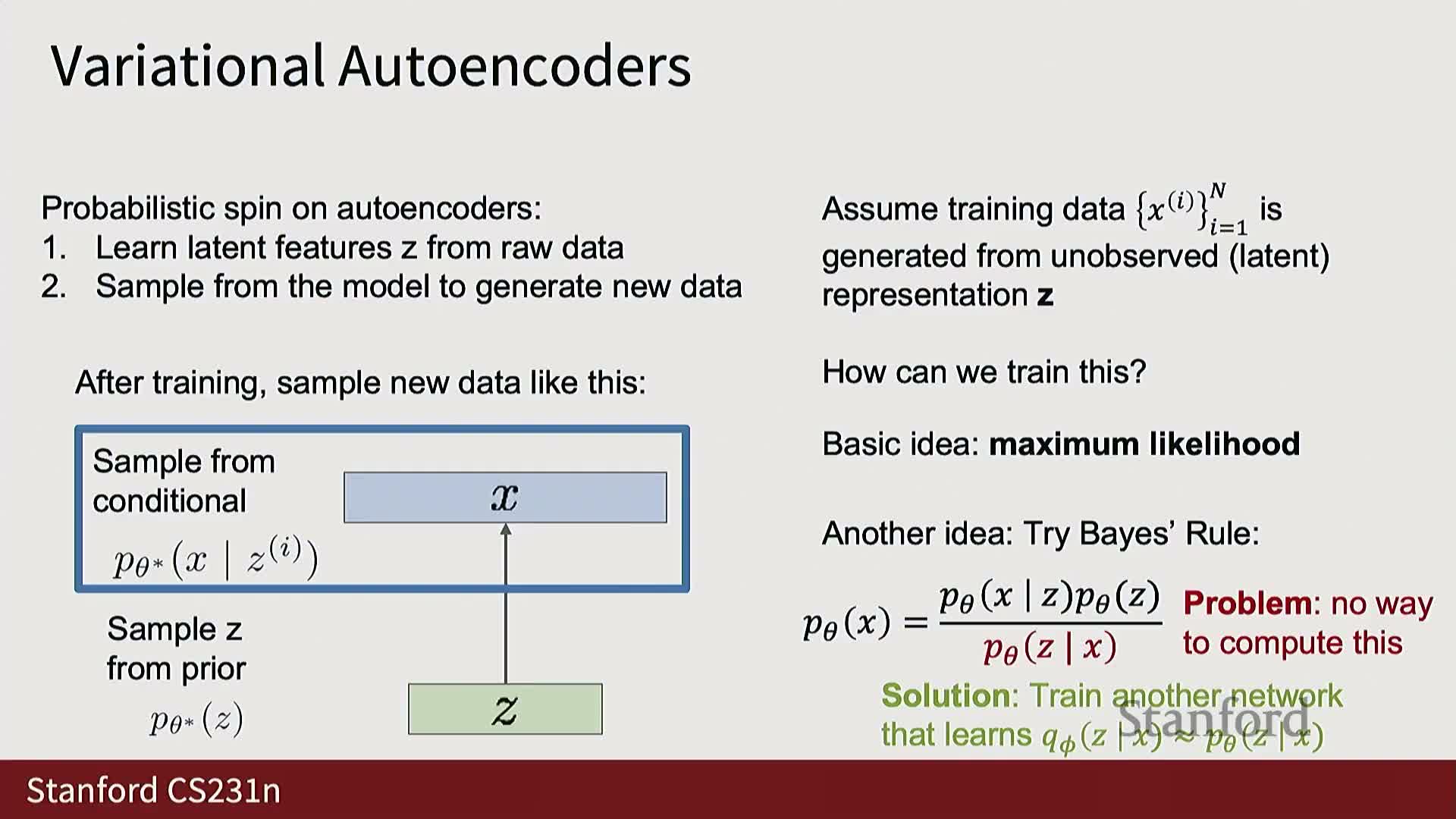
Variational autoencoders posit a joint model p_theta(X,Z) = p_theta(X|Z) p(Z) where p(Z) is a simple prior (typically unit Gaussian) and p_theta(X|Z) is a decoder neural network defining a conditional distribution over X given Z.
Inference and approximation:
-
The true posterior **p_theta(Z X)** is intractable for expressive decoders, so VAEs introduce an approximate posterior **q_phi(Z X)** implemented by an encoder network.
- The encoder outputs parameters (mean and diagonal covariance) of a Gaussian over Z; the decoder outputs parameters of a tractable conditional (often a diagonal Gaussian) for X given Z.
- Designing encoder and decoder outputs as Gaussian parameters enables closed-form KL computations between diagonal Gaussians and supports efficient backpropagation via the reparameterization trick:
z = mu_phi(x) + sigma_phi(x) * epsilon with epsilon ~ N(0,I), allowing gradient flow through sampling.
The evidence lower bound (ELBO) provides a tractable training objective that trades exact likelihood for a computable lower bound
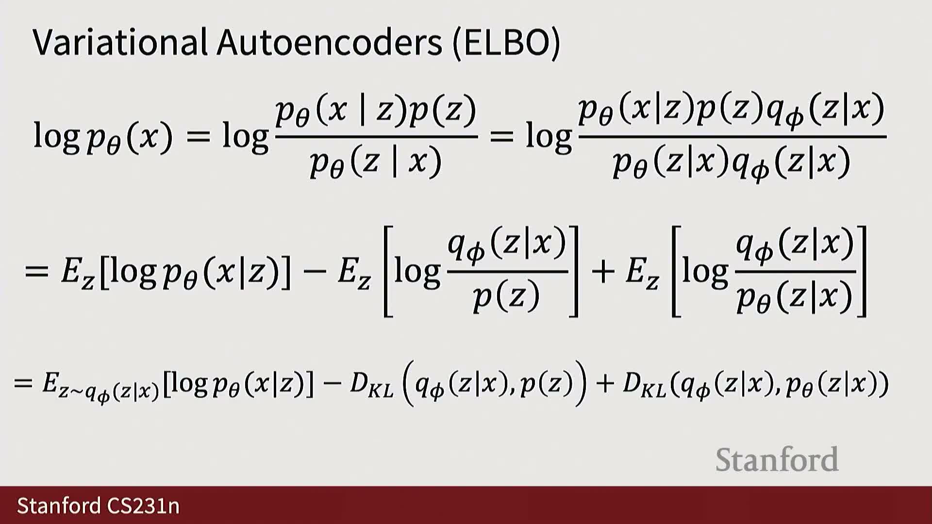
Direct maximization of the marginal log-likelihood log p_theta(X) requires integrating out Z, which is intractable for expressive neural decoders. The ELBO (evidence lower bound) is derived by introducing q_phi(Z|X) and applying Jensen’s inequality to produce a lower bound on log p_theta(X).
ELBO decomposition and interpretation:
- Two interpretable terms:
-
Expected reconstruction term: E_{z~q_phi(z x)}[log p_theta(x z)] — encourages accurate reconstructions when sampling z from the encoder.
-
KL divergence term: KL[q_phi(z x) p(z)] — regularizes the approximate posterior toward the chosen prior.
-
- Maximizing the ELBO jointly updates encoder parameters phi and decoder parameters theta.
- The KL term enforces encoded latents align with the prior (enabling sampling), while the reconstruction term preserves information needed to reconstruct x — a tradeoff between fidelity and latent-space regularity.
VAE training uses the reparameterization trick, balances reconstruction and prior terms, and enables latent interpolation and sampling
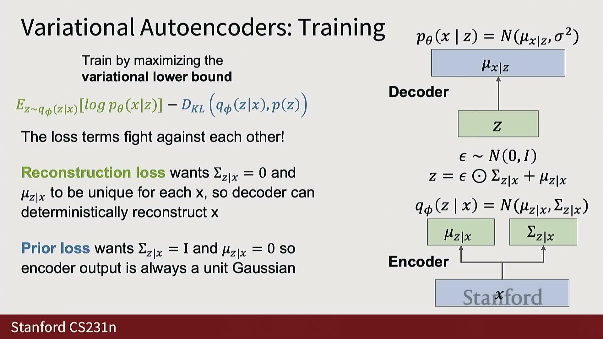
In practice the encoder outputs mu_phi(x) and log-variance parameters for a diagonal Gaussian q_phi(z|x); training samples z are drawn via the reparameterization z = mu + sigma * epsilon so gradients propagate through sampling.
Training and sampling details:
- The training objective is the negative ELBO (or equivalently maximize ELBO), combining:
- the expected log-likelihood (often implemented as an L2-like reconstruction under Gaussian decoder noise), and
- the KL divergence to the prior.
- These two terms compete: the reconstruction term encourages expressive, data-specific means and small variances, while the KL term pulls posteriors toward the unit Gaussian prior.
-
After training, sampling is straightforward: draw z ~ p(z) (the prior) and compute x ~ p_theta(x z) (often using the decoder mean).
- The diagonal Gaussian latent structure commonly yields semantically meaningful directions in latent space enabling smooth interpolation between samples.
- Important implementation choices include decoder likelihood family, variance handling (fixed vs learned), and KL weighting strategies to control the tradeoff between sample quality and latent regularity.
Enjoy Reading This Article?
Here are some more articles you might like to read next: