Stanford CS231N Deep Learning for Computer Vision| Spring 2025 | Lecture 14- Generative Models 2
- Likelihood-based explicit-density models (autoregressive models and variational autoencoders) estimate data densities directly and optimize likelihood objectives
- Implicit-density models for generative modeling do not yield explicit P(X) values but permit sampling from an induced generator distribution
- Generative adversarial networks use a discriminator network to enforce distributional alignment between the generator-induced distribution and the data distribution
- The GAN training objective is a minimax game between generator and discriminator optimized via alternating gradient updates
- The GAN value V is not a straightforward scalar loss for monitoring progress, and GAN optimization is fundamentally unstable
- GANs exhibit difficult early-stage learning dynamics and a practical non-saturating loss modification improves generator gradients
- Under idealized assumptions the GAN objective has a provable optimum at PG = Pdata via the optimal discriminator, but practical caveats limit this guarantee
- GAN architectures evolved from DCGAN to StyleGAN, and well-trained GANs can learn smooth latent-space interpolations
- GANs trade high sample quality for difficult and brittle training, common failure modes include mode collapse and memorization
- Diffusion models replace adversarial training with iterative denoising of samples corrupted by increasing noise levels
- Rectified flow is a diffusion-style formulation that trains a network to predict the velocity vector from clean data to noise on interpolated samples
- Sampling from rectified-flow diffusion models iteratively updates a noisy sample by stepping along predicted velocity vectors from high to low noise levels
- Conditional diffusion models incorporate auxiliary inputs (e.g., class labels or text) and classifier-free guidance is a practical technique to amplify conditioning at sampling time
- Noise schedules and sampling density across noise levels critically affect diffusion training and inference difficulty
- Latent diffusion models scale diffusion to high-resolution data by running diffusion in a compressed latent space produced by an encoder-decoder (typically a VAE)
- Modern diffusion architectures frequently use transformer-based denoisers with mechanisms for embedding time and conditioning inputs
- Text-to-image pipelines use a frozen or pre-trained text encoder to provide conditioning embeddings that guide a latent diffusion model
- Text-to-video extends latent diffusion to an additional temporal dimension, greatly increasing sequence length and computational cost
- Distillation methods accelerate diffusion sampling by learning to approximate many-step denoising with far fewer steps, trading compute for potential quality loss
- Multiple rigorous formalisms underpin diffusion models—latent-variable ELBOs, score-matching, and SDE-based perspectives—which yield related algorithms
- Autoregressive models on discrete latents and combined pipelines summarize the modern generative modeling toolkit
Likelihood-based explicit-density models (autoregressive models and variational autoencoders) estimate data densities directly and optimize likelihood objectives
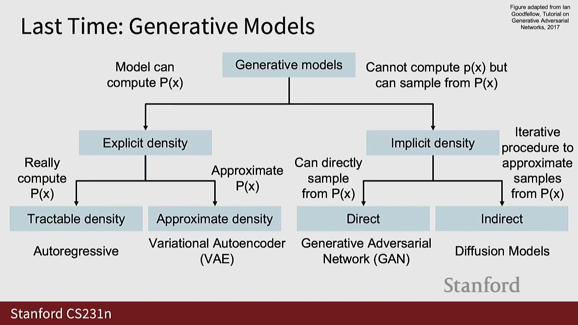
Explicit-density generative models produce or approximate an explicit probability density P(X) and are typically trained with likelihood-based objectives.
Autoregressive models factorize the joint density as a product of conditional distributions over a sequence (e.g., pixels or sub-pixel discrete values) and model those conditionals with sequence models such as RNNs or Transformers.
- Key properties:
- Enable exact likelihood evaluation.
- Support straightforward sampling via ancestral sampling.
- Enable exact likelihood evaluation.
Variational autoencoders (VAEs) introduce an encoder q(z|x) and a decoder p(x|z) and optimize a variational lower bound on the marginal likelihood by jointly training encoder and decoder.
- The encoder outputs a distribution over latent codes; the decoder maps latents back to data.
- Tradeoffs and considerations:
- The VAE objective trades exact likelihood for a tractable lower bound (the ELBO).
- VAEs produce useful latent representations for downstream tasks.
- They require careful selection of the approximate posterior, priors, and decoder parameterization to achieve good samples and representations.
- The VAE objective trades exact likelihood for a tractable lower bound (the ELBO).
Implicit-density models for generative modeling do not yield explicit P(X) values but permit sampling from an induced generator distribution
Implicit-density models dispense with computing explicit density values and instead define a sampling procedure that induces a distribution PG over data; the model provides no tractable P(X) but allows drawing synthetic samples.
Typical construction:
- A simple prior p(z) (commonly a unit Gaussian).
- A parameterized generator G(z) that maps latent draws to data-space samples. Modifying G changes the induced distribution PG.
Training objective:
- Adjust G so that the induced PG approximates the unknown data distribution Pdata, enabling realistic sample generation even without access to density evaluations.
Generative adversarial networks use a discriminator network to enforce distributional alignment between the generator-induced distribution and the data distribution
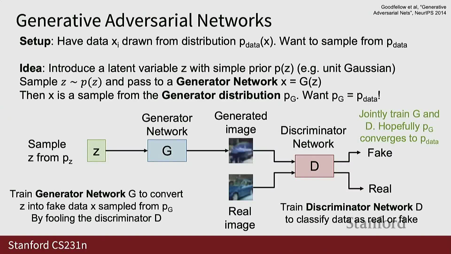
A generative adversarial network (GAN) pairs a generator G with a discriminator D(x) that outputs the probability a sample x is real versus generated.
- The discriminator is a learned, differentiable test the generator tries to fool.
- Typical objectives:
- Discriminator maximizes log-probabilities for real samples and log(1 − D(G(z))) for generated samples.
- Generator is commonly trained to maximize D(G(z)), or equivalently to minimize −log D(G(z)) in the non-saturating variant.
- Discriminator maximizes log-probabilities for real samples and log(1 − D(G(z))) for generated samples.
- Training dynamics:
- Gradients flow from the discriminator through generated samples back into the generator parameters, enabling end-to-end training.
- Gradients flow from the discriminator through generated samples back into the generator parameters, enabling end-to-end training.
- Conceptual shift:
- The adversarial setup turns distribution matching into a two-player minimax game rather than explicit density estimation.
- The adversarial setup turns distribution matching into a two-player minimax game rather than explicit density estimation.
The GAN training objective is a minimax game between generator and discriminator optimized via alternating gradient updates
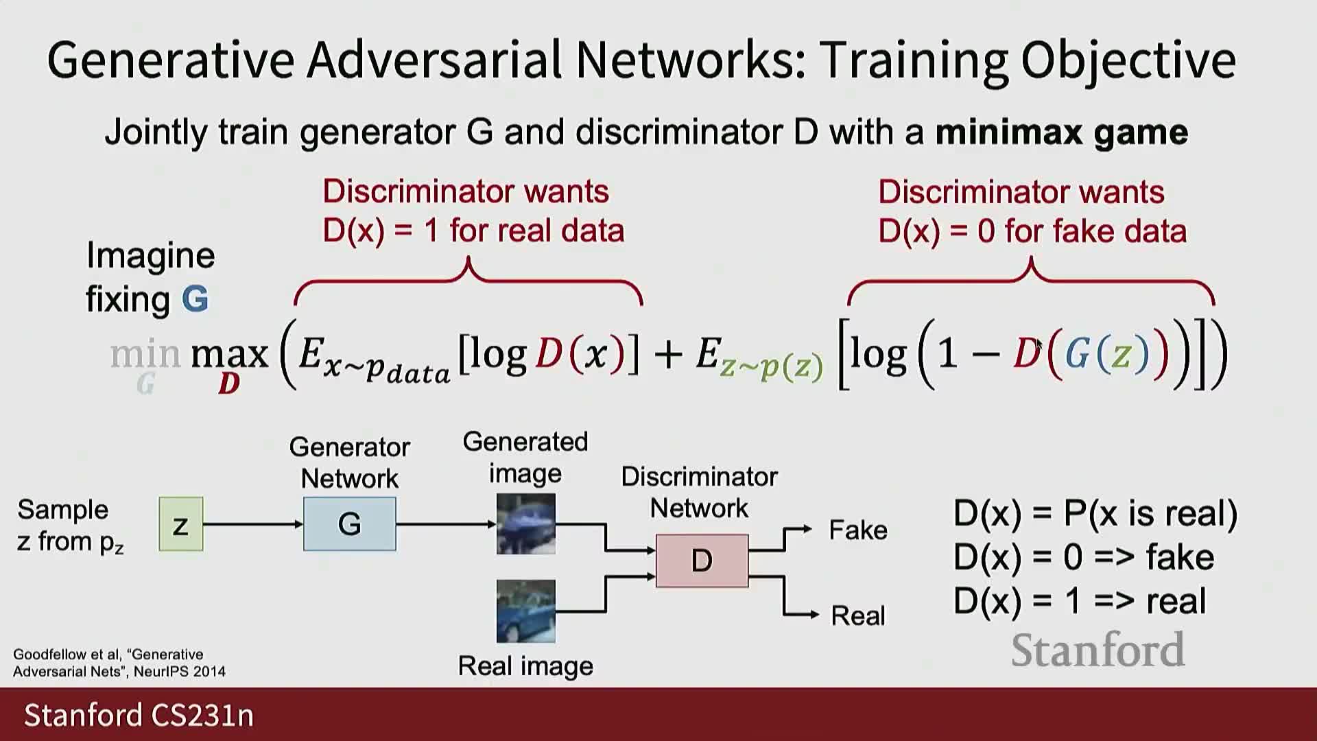
GAN training formalizes the adversarial process as an inner maximization over the discriminator and an outer minimization over the generator for a value function V(G, D) that aggregates expected log-probabilities on real and generated samples.
- Optimization pattern:
- The discriminator performs gradient ascent on its parameters to maximize V.
- The generator performs gradient descent on its parameters to minimize V.
- The discriminator performs gradient ascent on its parameters to maximize V.
- Implementation detail:
- Typically implemented with alternating optimization steps (e.g., multiple discriminator updates per generator update or vice versa).
- Typically implemented with alternating optimization steps (e.g., multiple discriminator updates per generator update or vice versa).
- Assumptions and caveats:
- This procedure relies on backpropagating discriminator gradients through generated samples and assumes sufficient model capacity and stable optimization dynamics for the game to reach an equilibrium where PG ≈ Pdata.
- This procedure relies on backpropagating discriminator gradients through generated samples and assumes sufficient model capacity and stable optimization dynamics for the game to reach an equilibrium where PG ≈ Pdata.
The GAN value V is not a straightforward scalar loss for monitoring progress, and GAN optimization is fundamentally unstable
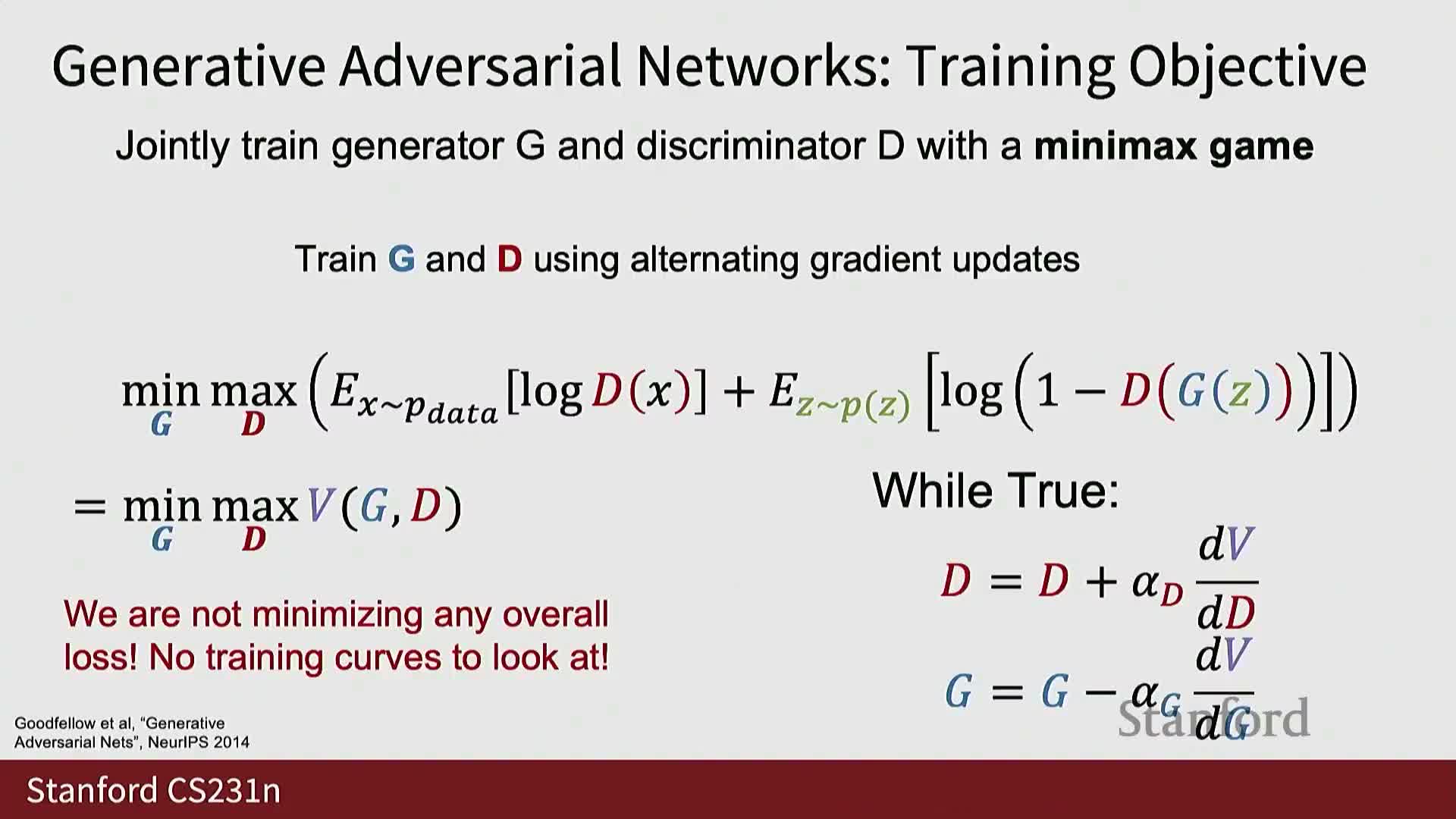
The scalar value V of the minimax game does not behave like a conventional loss metric because its magnitude depends on the relative strengths and equilibria of the generator and discriminator rather than a univariate measure of sample quality.
- Practical consequences:
- Different combinations of generator and discriminator performance can yield similar V values, so tracking V (or the separate generator/discriminator objectives) often gives little diagnostic information about whether PG is approaching Pdata.
- Optimization is inherently unstable because it attempts simultaneous maximization and minimization of a shared objective across interacting parameter sets, producing:
-
Nonstationary dynamics.
- High sensitivity to hyperparameters.
- Frequent need for extensive heuristics to stabilize training.
-
Nonstationary dynamics.
- Different combinations of generator and discriminator performance can yield similar V values, so tracking V (or the separate generator/discriminator objectives) often gives little diagnostic information about whether PG is approaching Pdata.
GANs exhibit difficult early-stage learning dynamics and a practical non-saturating loss modification improves generator gradients
At initialization a randomly parameterized generator produces near-random samples that are trivial for the discriminator to separate from real data.
- Effect on gradients:
- Discriminator outputs near zero for generated samples cause very small gradients for the generator under the naive log(1 − D(G(z))) objective.
- Discriminator outputs near zero for generated samples cause very small gradients for the generator under the naive log(1 − D(G(z))) objective.
- Common remedy:
- Use the non-saturating objective and train the generator to minimize −log D(G(z)), which provides stronger gradients when the discriminator is confident and accelerates early learning.
- Use the non-saturating objective and train the generator to minimize −log D(G(z)), which provides stronger gradients when the discriminator is confident and accelerates early learning.
- Remaining coupling:
- Training remains end-to-end and the only signal to the generator comes through discriminator gradients, which can exacerbate instability despite the heuristic improvement.
- Training remains end-to-end and the only signal to the generator comes through discriminator gradients, which can exacerbate instability despite the heuristic improvement.
Under idealized assumptions the GAN objective has a provable optimum at PG = Pdata via the optimal discriminator, but practical caveats limit this guarantee
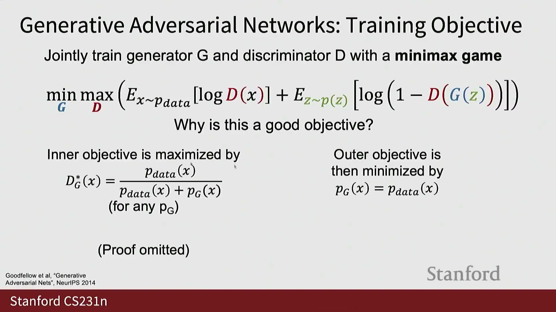
The GAN minimax game admits an analytic solution for the inner maximization: for a fixed generator the optimal discriminator can be expressed in closed form as a function of Pdata and PG.
- Theoretical implication:
- Substituting this optimal discriminator into the value function yields an objective minimized when PG = Pdata, providing a principled existence proof that the global optimum corresponds to distributional matching.
- Substituting this optimal discriminator into the value function yields an objective minimized when PG = Pdata, providing a principled existence proof that the global optimum corresponds to distributional matching.
- Practical limitations:
- This result requires infinite model capacity and access to true densities or infinite data.
- It offers no guarantees of convergence under gradient-based training with finite-capacity networks or finite samples.
- Consequently the theoretical justification is limited in operational utility without further constraints and careful engineering.
- This result requires infinite model capacity and access to true densities or infinite data.
GAN architectures evolved from DCGAN to StyleGAN, and well-trained GANs can learn smooth latent-space interpolations
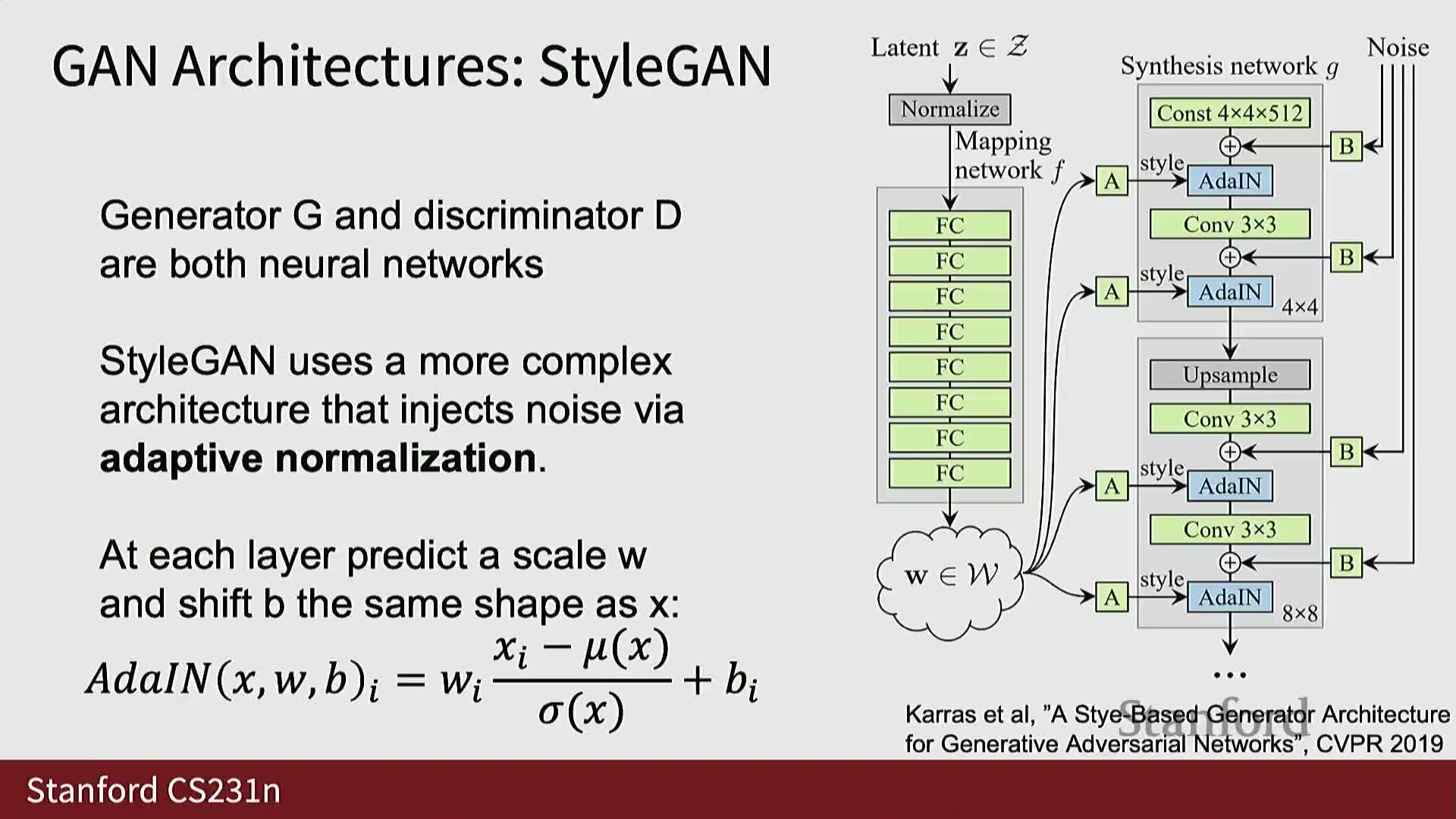
Convolutional GAN architectures such as DCGAN demonstrated early impactful image-generation results by combining convolutional generator and discriminator blocks.
- Architectural advances:
- Later designs like StyleGAN introduced more sophisticated generator parameterizations and normalization techniques that improved sample fidelity and controllability.
- Later designs like StyleGAN introduced more sophisticated generator parameterizations and normalization techniques that improved sample fidelity and controllability.
- Latent-space properties:
- Well-optimized GAN generators often yield a learned latent manifold with smooth semantic interpolations — linear or nonlinear paths in latent space produce smoothly varying decoded images, indicating meaningful structure in the representation.
- Well-optimized GAN generators often yield a learned latent manifold with smooth semantic interpolations — linear or nonlinear paths in latent space produce smoothly varying decoded images, indicating meaningful structure in the representation.
- Practical note:
- These advances underpin many high-fidelity image generation systems but require delicate training and hyperparameter tuning.
- These advances underpin many high-fidelity image generation systems but require delicate training and hyperparameter tuning.
GANs trade high sample quality for difficult and brittle training, common failure modes include mode collapse and memorization
GANs can produce sharp, photorealistic samples when carefully tuned, but they suffer notable practical drawbacks.
- Common failure modes:
-
Training instability and sensitivity to architectural/optimization choices.
- Catastrophic failures such as exploding losses or NaNs.
-
Mode collapse, where the generator maps many latents to a small set of outputs or memorizes training samples.
-
Training instability and sensitivity to architectural/optimization choices.
- Mode collapse specifics:
- Can manifest as the generator ignoring the latent z input and producing a limited set of outputs, leading to poor diversity and a degenerate PG.
- Can manifest as the generator ignoring the latent z input and producing a limited set of outputs, leading to poor diversity and a degenerate PG.
- Broader implication:
- These failure modes combined with the lack of reliable scalar diagnostics historically made GANs challenging to scale reliably, motivating alternative generative paradigms.
- These failure modes combined with the lack of reliable scalar diagnostics historically made GANs challenging to scale reliably, motivating alternative generative paradigms.
Diffusion models replace adversarial training with iterative denoising of samples corrupted by increasing noise levels
Diffusion-based generative models construct a continuum of corrupted versions of data by progressively adding noise parameterized by a noise level t ∈ [0,1] (t = 0 is clean data, t = 1 is pure noise), and train the model to perform small denoising steps at intermediate noise levels.
- Training setup:
- A neural network receives a noisy sample and a noise-level embedding and is optimized to estimate either:
- The clean signal, or
- The added noise, or
- Another task-specific target.
- The clean signal, or
- A neural network receives a noisy sample and a noise-level embedding and is optimized to estimate either:
- Inference:
- Starts from pure noise and applies the denoiser iteratively across decreasing t to synthesize a clean sample.
- Starts from pure noise and applies the denoiser iteratively across decreasing t to synthesize a clean sample.
- Advantages:
- The iterative denoising framework yields tractable training losses that correlate with sample quality and supports both continuous and discrete-time formulations.
- The iterative denoising framework yields tractable training losses that correlate with sample quality and supports both continuous and discrete-time formulations.
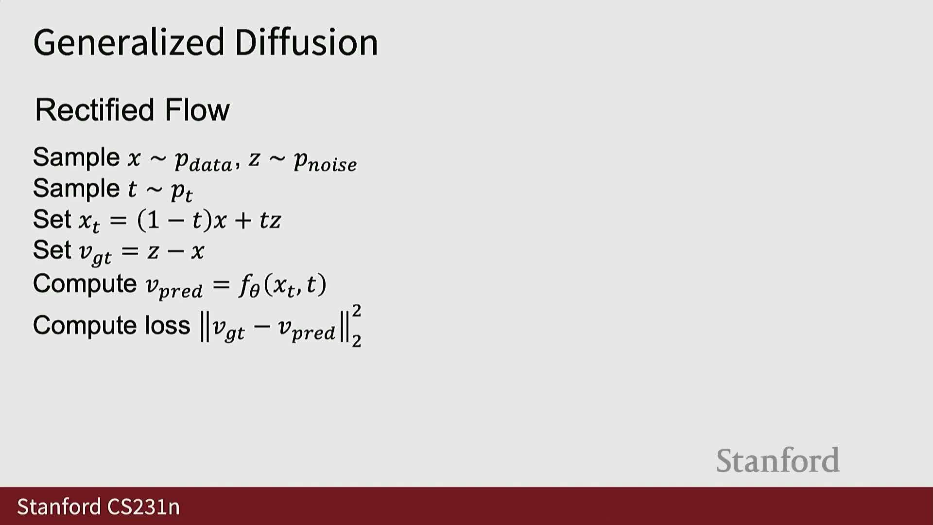
Rectified flow is a diffusion-style formulation that trains a network to predict the velocity vector from clean data to noise on interpolated samples
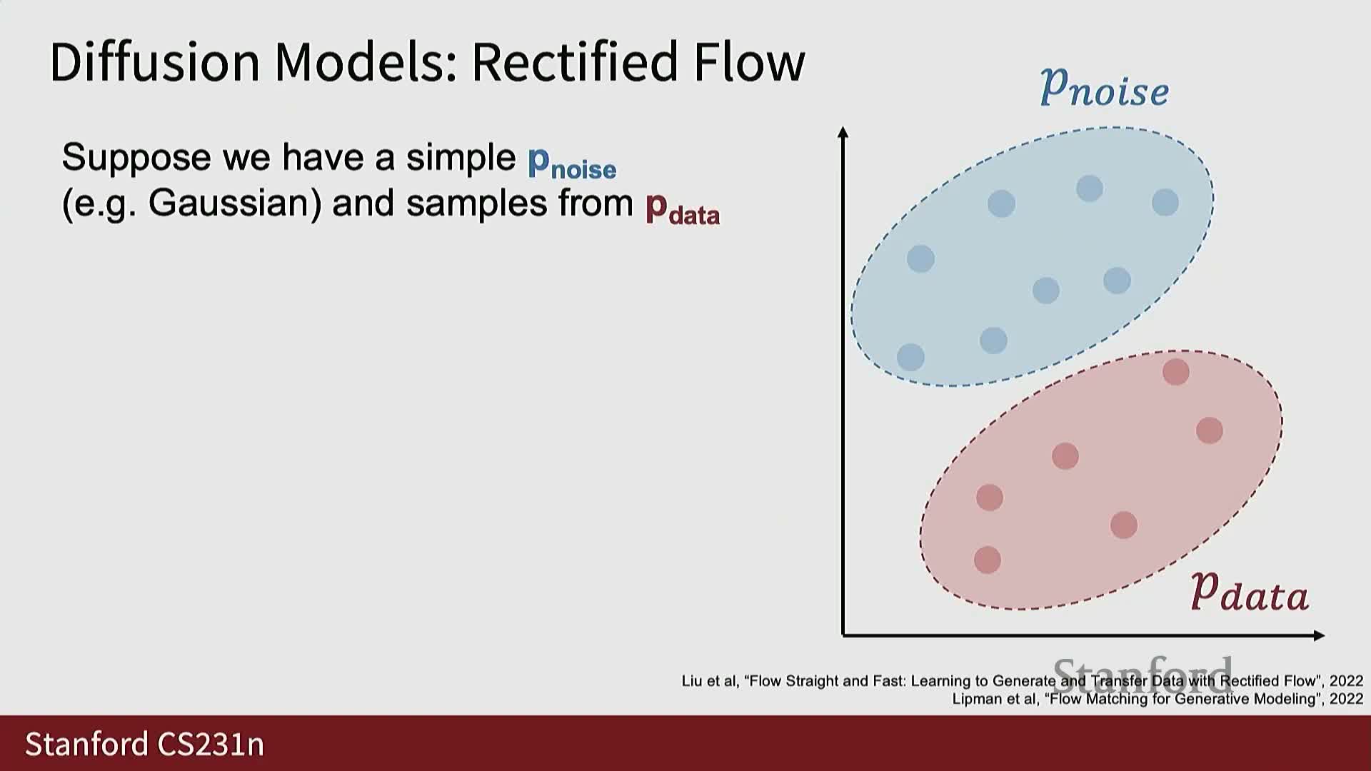
Rectified flow formalizes a geometric denoising task via linear interpolation between data and noise.
- Setup and target:
- Sample data point x ∼ Pdata and independent noise point z ∼ Pz.
- Choose t uniformly in [0,1] and form x_t as the linear interpolation between x and z at t.
- Train a model f_θ(x_t, t) to predict the ground-truth velocity vector v = z − x (or an equivalent linear target) using a mean squared error (MSE) loss.
- Sample data point x ∼ Pdata and independent noise point z ∼ Pz.
- Outcome:
- The network learns a vector field that points noisy samples toward cleaner regions of the data manifold and can be used for iterative sample refinement at inference.
- The network learns a vector field that points noisy samples toward cleaner regions of the data manifold and can be used for iterative sample refinement at inference.
Sampling from rectified-flow diffusion models iteratively updates a noisy sample by stepping along predicted velocity vectors from high to low noise levels
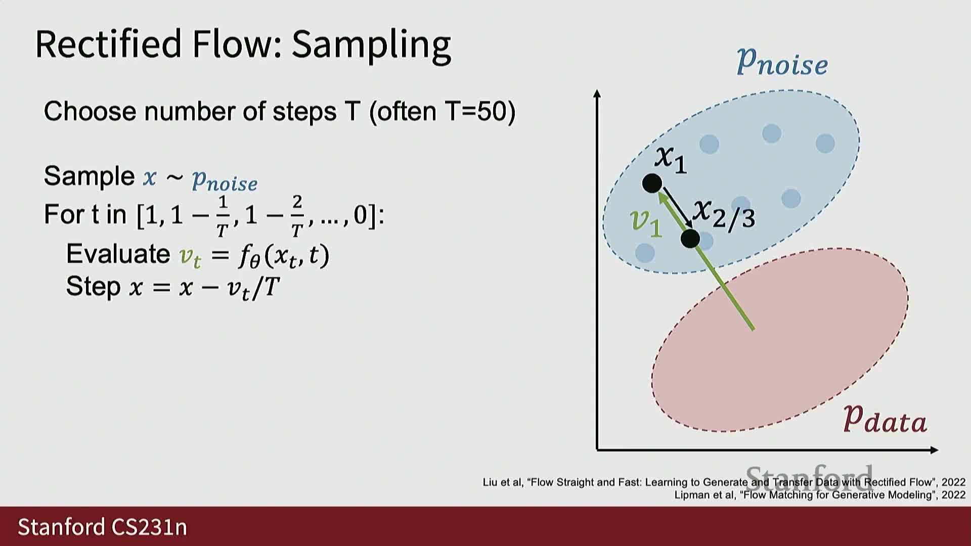
Inference for rectified flow and related denoising samplers proceeds iteratively from noise toward data-like samples.
- Draw an initial sample from the prior noise distribution.
- Select a sequence of noise levels that march from full noise toward zero.
- At each step:
- Use the model to predict a velocity (or denoising direction) at the current x_t and t.
- Take a small step along the predicted vector to obtain a slightly denoised sample.
- Use the model to predict a velocity (or denoising direction) at the current x_t and t.
- Repeat the predict–update cycle across the chosen schedule until reaching a low-noise or clean sample.
- The full trajectory integrates many small denoising steps into a path from noise to data and is analogous to integrating a flow or score-based SDE; performance depends on the number of steps, step sizes, and the noise-level schedule used in training and sampling.
Conditional diffusion models incorporate auxiliary inputs (e.g., class labels or text) and classifier-free guidance is a practical technique to amplify conditioning at sampling time
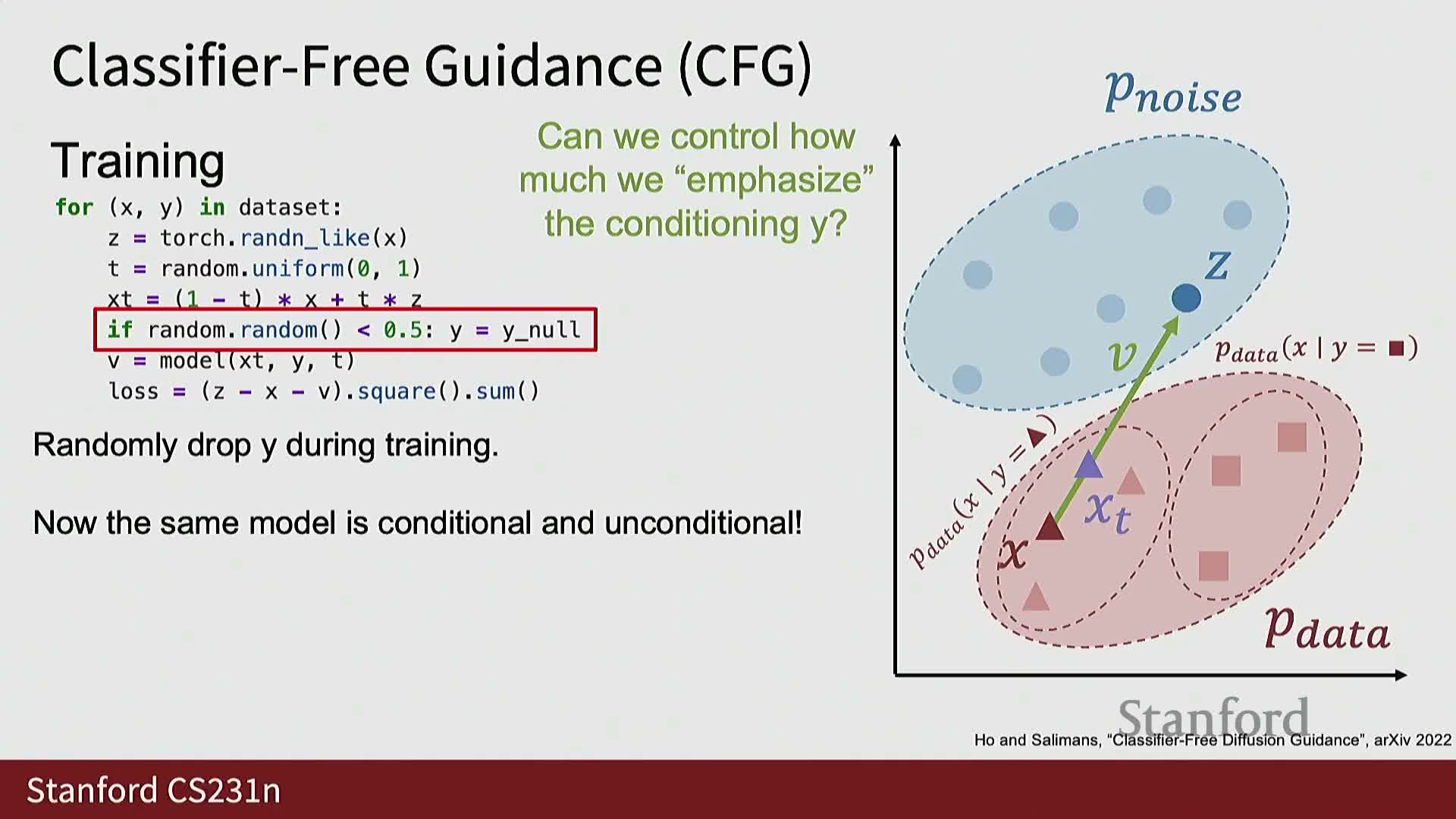
Conditioning signals Y are incorporated by providing Y as an additional input to the denoising network so the model learns conditional velocity or score fields that concentrate probability mass on data consistent with Y.
-
Classifier-free guidance:
- Train the model to handle both conditioned and unconditioned inputs by randomly dropping the conditioning during training (commonly 50% of the time). The network thus learns:
- A conditional vector field v_cond, and
- An unconditional vector field v_uncond.
- A conditional vector field v_cond, and
- During sampling combine the two predictions with a guidance weight w:
-
v_cfg = v_uncond + w * (v_cond − v_uncond).
-
v_cfg = v_uncond + w * (v_cond − v_uncond).
- This enables control over adherence to the conditioning signal at the cost of evaluating the model twice per step.
- Train the model to handle both conditioned and unconditioned inputs by randomly dropping the conditioning during training (commonly 50% of the time). The network thus learns:
Noise schedules and sampling density across noise levels critically affect diffusion training and inference difficulty
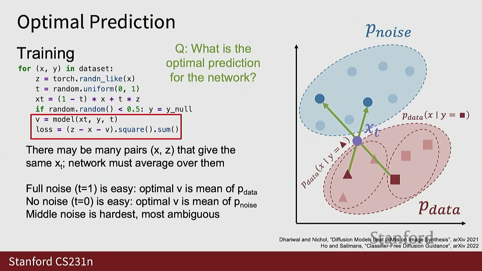
The choice of the noise-level distribution P(t) and the functional mapping that blends clean data and noise into x_t shape the learning difficulty across t.
- Observations:
- Uniform sampling of t weights all noise levels equally, but intermediate t values often present the hardest inverse problems because multiple (x, z) pairs can map to the same x_t.
- Uniform sampling of t weights all noise levels equally, but intermediate t values often present the hardest inverse problems because multiple (x, z) pairs can map to the same x_t.
- Practical schedules:
- Practitioners use nonuniform noise schedules (e.g., log-normal or shifted schedules) that emphasize informative or difficult intermediate regions while down-weighting trivial endpoints.
- Practitioners use nonuniform noise schedules (e.g., log-normal or shifted schedules) that emphasize informative or difficult intermediate regions while down-weighting trivial endpoints.
- Scaling consideration:
- Schedule design becomes more important for high-resolution data, where spatial correlations change how information is destroyed by noise.
- Schedule design becomes more important for high-resolution data, where spatial correlations change how information is destroyed by noise.
Latent diffusion models scale diffusion to high-resolution data by running diffusion in a compressed latent space produced by an encoder-decoder (typically a VAE)
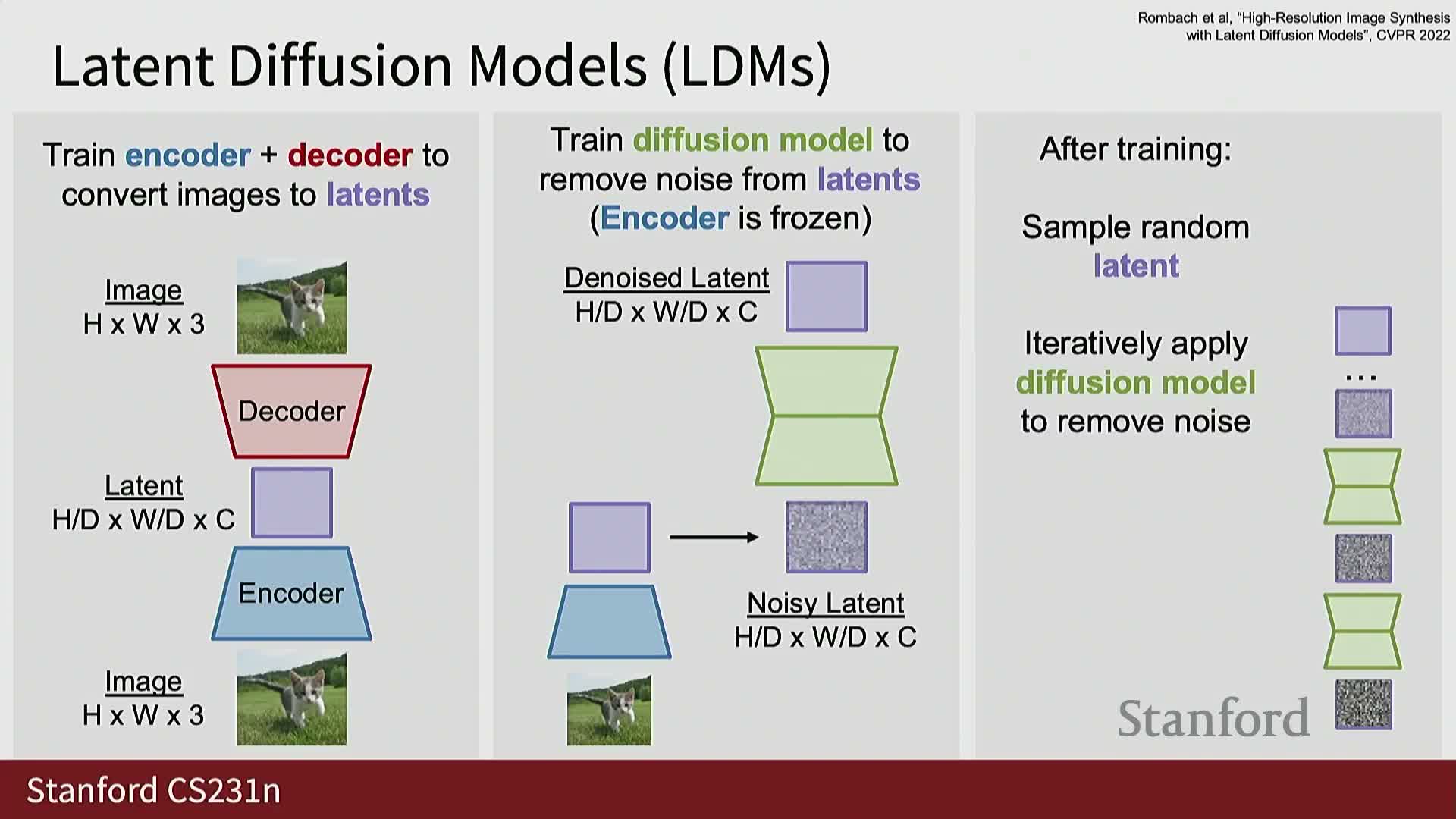
Latent diffusion first trains or adopts an encoder that maps high-dimensional images into a lower-dimensional latent representation and a decoder that reconstructs images from latents; diffusion is then applied in latent space rather than on raw pixels.
- Pipeline notes:
- Latents typically use spatial downsampling with increased channel depth.
- Because standalone VAEs can produce blurry reconstructions, modern pipelines augment the decoder with additional discriminators or apply adversarial and perceptual losses to improve visual fidelity.
- Common approach: combine VAE-style compression with GAN-style discriminators, train the latent diffusion model on these learned latents while freezing the encoder.
- Latents typically use spatial downsampling with increased channel depth.
- Benefits:
- The two-stage approach dramatically reduces computation and sequence length during diffusion training and sampling, enabling high-resolution image and video synthesis while leveraging components from multiple generative paradigms.
- The two-stage approach dramatically reduces computation and sequence length during diffusion training and sampling, enabling high-resolution image and video synthesis while leveraging components from multiple generative paradigms.
Modern diffusion architectures frequently use transformer-based denoisers with mechanisms for embedding time and conditioning inputs
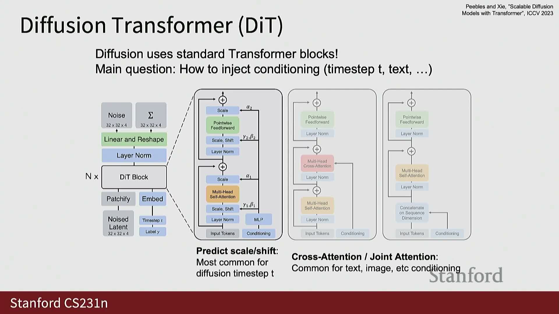
Diffusion transformers (DiTs) apply standard transformer blocks to model noisy latents as sequences, leveraging attention for long-range spatial and temporal interactions.
- Architectural details:
- Time-step embeddings are commonly injected via learned scale-and-shift parameters that modulate intermediate activations.
- Conditioning modalities such as text are provided by:
- Concatenating token sequences and using cross-attention, or
- Using joint-attention mechanisms that fuse modalities.
- Concatenating token sequences and using cross-attention, or
- Time-step embeddings are commonly injected via learned scale-and-shift parameters that modulate intermediate activations.
- Advantage:
- This modularity simplifies extending diffusion models to multimodal conditional generation while maintaining high representational capacity for both images and videos.
- This modularity simplifies extending diffusion models to multimodal conditional generation while maintaining high representational capacity for both images and videos.
Text-to-image pipelines use a frozen or pre-trained text encoder to provide conditioning embeddings that guide a latent diffusion model
Text-to-image generation pipelines embed a text prompt with a pre-trained text encoder (e.g., CLIP, T5) and feed the resulting embeddings as conditioning into a latent diffusion denoiser together with noisy latents and a time embedding.
- Flow:
- The denoiser iteratively transforms noise-distributed latents toward conditioned latent samples.
- A decoder (trained with perceptual or adversarial losses) converts final latents back to pixels.
- The denoiser iteratively transforms noise-distributed latents toward conditioned latent samples.
- Practical notes:
- The text encoder is often frozen to leverage large-scale pretraining.
- Scaled systems operate on long sequences of image tokens (e.g., thousands of tokens) and use large transformers to achieve state-of-the-art conditional image synthesis quality.
- The text encoder is often frozen to leverage large-scale pretraining.
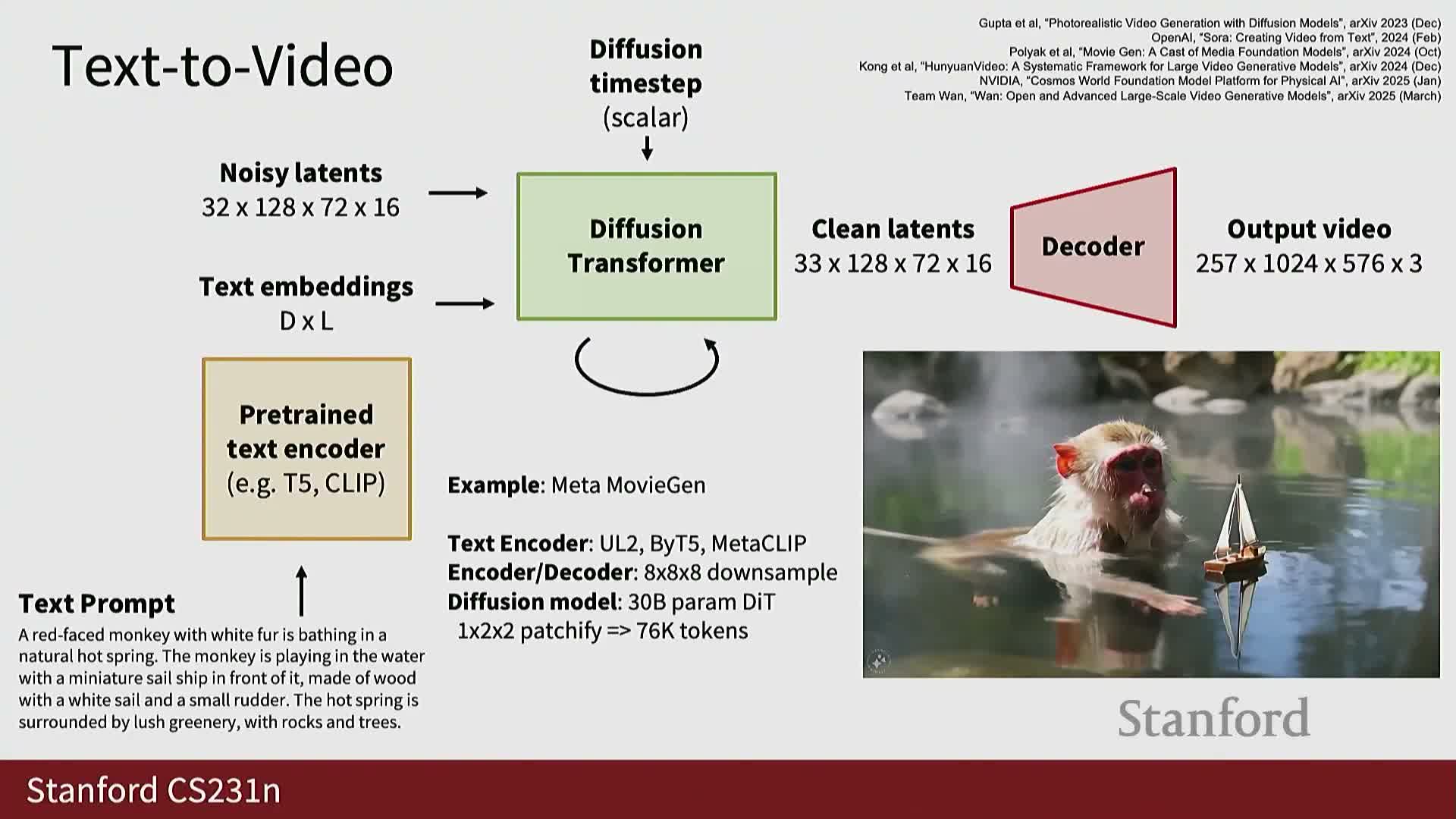
Text-to-video extends latent diffusion to an additional temporal dimension, greatly increasing sequence length and computational cost

Text-to-video diffusion models extend the conditional latent-diffusion pipeline with latents that include an explicit time axis in addition to spatial axes and use spatiotemporal encoder/decoder modules that down- and up-sample across both space and time.
- Computational challenge:
- Sequence lengths can be orders of magnitude larger than image-token sequences, driving the primary computational cost in training and inference.
- Addressing this requires architectural and efficiency innovations (e.g., sparse attention, factorized temporal processing, or compression).
- Sequence lengths can be orders of magnitude larger than image-token sequences, driving the primary computational cost in training and inference.
- Recent progress:
- Large-scale video diffusion systems have adopted transformer-based denoisers and scalability techniques to achieve high-quality text-to-video synthesis, catalyzing rapid research and product development in video generative modeling.
- Large-scale video diffusion systems have adopted transformer-based denoisers and scalability techniques to achieve high-quality text-to-video synthesis, catalyzing rapid research and product development in video generative modeling.
Distillation methods accelerate diffusion sampling by learning to approximate many-step denoising with far fewer steps, trading compute for potential quality loss
Diffusion sampling is iterative and computationally expensive because it requires tens to hundreds of model evaluations per sample; distillation methods compress this iterative procedure by training a model (or sequence of models) to emulate multiple denoising steps with fewer evaluations.
- Distillation approaches:
- Range from multistep to single-step approximations.
- Aim to preserve sample quality while drastically reducing latency.
- Range from multistep to single-step approximations.
- Trade-offs:
- Achieving high-fidelity compressed samplers is an active research area that balances inference speed, sample quality, and additional training complexity.
- Achieving high-fidelity compressed samplers is an active research area that balances inference speed, sample quality, and additional training complexity.
Multiple rigorous formalisms underpin diffusion models—latent-variable ELBOs, score-matching, and SDE-based perspectives—which yield related algorithms
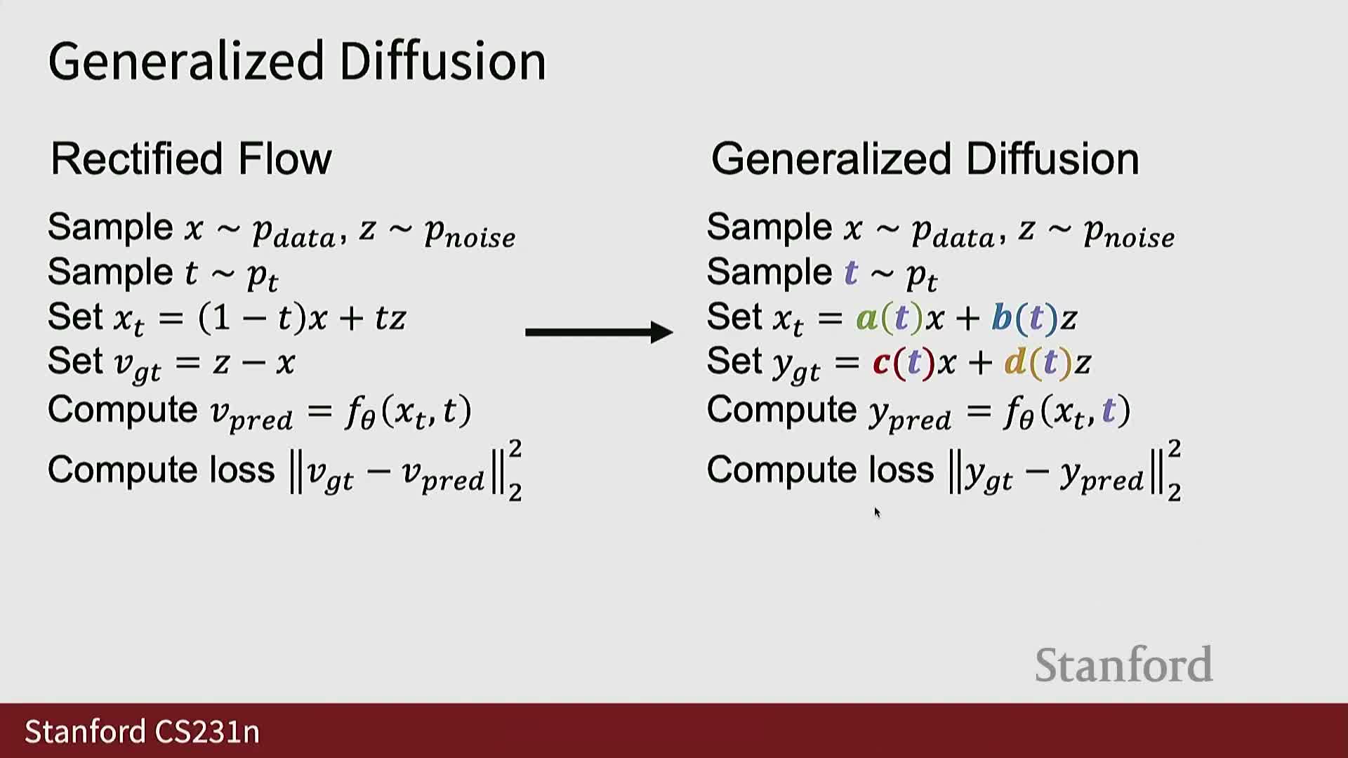
Diffusion models admit several mathematically distinct interpretations that converge to similar training and sampling procedures:
-
Latent-variable variational formulation — views corrupted intermediate samples as latent variables and derives ELBO-based objectives.
-
Score-matching perspective — trains networks to estimate the gradient of log-density (the score) for noised distributions and then uses Langevin or score-based samplers.
-
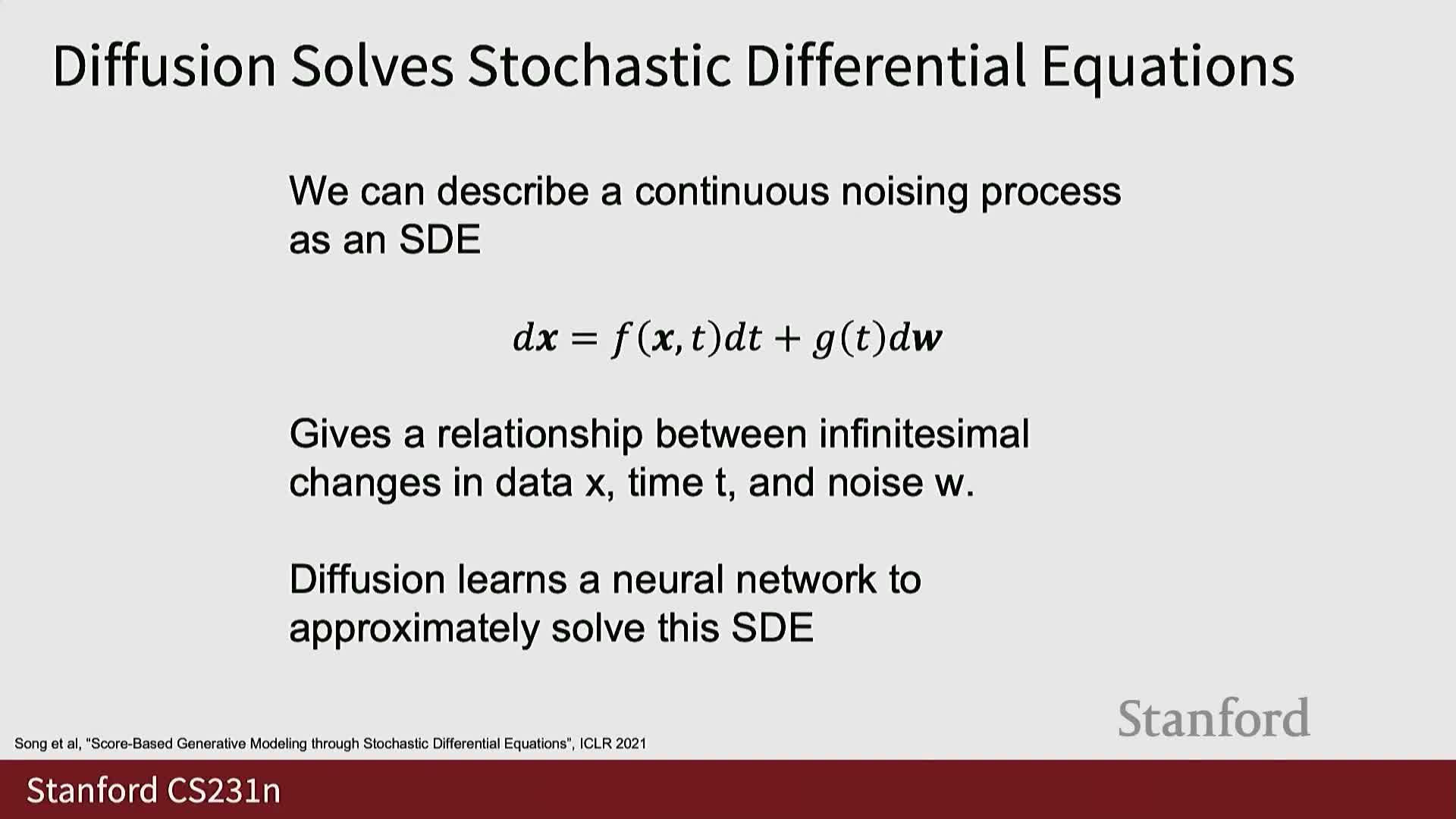
Stochastic differential equation (SDE) viewpoint — models forward noising and reverse denoising as continuous-time stochastic dynamics, enabling principled numerical integrators for sampling.
- Each perspective prescribes different choices for noise schedules, parameterizations, and discretization schemes and offers distinct theoretical and practical trade-offs exploited across the literature.
Autoregressive models on discrete latents and combined pipelines summarize the modern generative modeling toolkit
A prevalent modern recipe composes multiple generative paradigms into hybrid pipelines rather than relying on a single formulation.
- Typical components:
- A discrete or continuous variational autoencoder (VAE) to compress high-dimensional data into latents.
- An autoregressive or transformer-based model trained over discrete latents for likelihood modeling.
-
Diffusion denoisers as alternatives or complements depending on the task.
- A discrete or continuous variational autoencoder (VAE) to compress high-dimensional data into latents.
- Why combine models:
- Combining VAEs, GANs, autoregressive models, and diffusion models leverages complementary strengths:
- Efficient sampling.
- Controllable latents.
- High-fidelity samples.
- More stable training dynamics.
- Efficient sampling.
- Combining VAEs, GANs, autoregressive models, and diffusion models leverages complementary strengths:
- Takeaway:
- No single generative formulation dominates all tasks; hybrid systems achieve state-of-the-art results by orchestrating multiple models according to task requirements and resource constraints.
Enjoy Reading This Article?
Here are some more articles you might like to read next: