Stanford CS236- Deep Generative Models I 2023 I Lecture 2 - Background
- Course overview and objectives
- Problem statement: data are samples from an unknown distribution P_data
- Model family, loss function, and projection-based optimization
- Applications of learned probability distributions
- Representing probability distributions and the curse of dimensionality
- Discrete pixel modeling and combinatorial explosion in color spaces
- Binary image example and the exponential state space 2^n
- Assuming independence to reduce parameters and its limitations
- Chain rule (autoregressive factorization) for joint distributions
- Parameter explosion in naive autoregressive models and Markov assumptions
- Bayesian networks (directed graphical models) as structured factorization
- Example Bayesian network: modeling exam difficulty, intelligence, grades
- Using graphical models versus neural networks for conditional structure
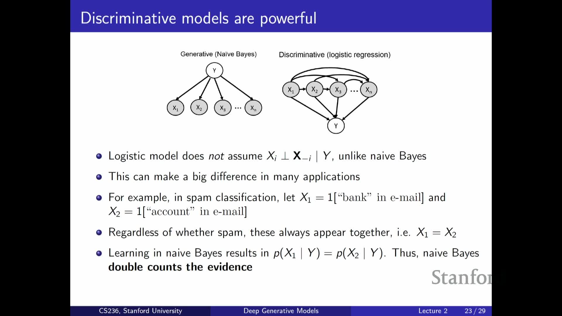
- Generative modeling applied to discriminative tasks: the Naive Bayes classifier
- Discriminative versus generative factorization and practical trade-offs
- Logistic regression as a functional parametrization of P(Y|X)
- Neural networks as richer functional parameterizations and deep autoregressive models
- Design choices for deep generative models: factorization, parameter tying, and assumptions
- Continuous variables, probability density functions, and latent-variable generative models (mixtures and VAEs)
Course overview and objectives
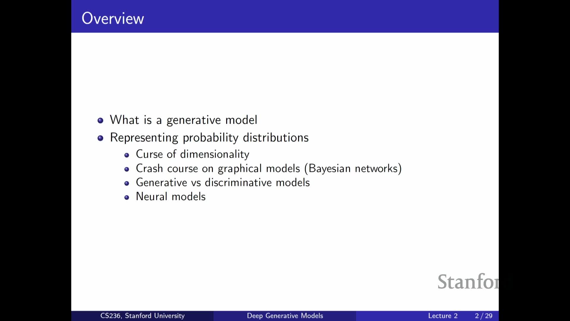
Provides a high-level roadmap for the lecture series that orients the listener around three goals:
- Define what we mean by generative models and introduce graphical models.
- Explain the generative vs. discriminative distinction and when each viewpoint is useful.
- Motivate using neural networks to combat the curse of dimensionality when modeling complex data like images and text.
The overview frames subsequent material around three components needed for generative modeling: data, a model family, and a similarity / loss metric.
- Changing any of these components yields different classes of generative models (for example: autoregressive models, diffusion models, GANs).
Taken together, this situates deep generative modeling as an exploration of representational and algorithmic choices that balance expressivity and tractability.
Problem statement: data are samples from an unknown distribution P_data

Defines the core problem: approximate an unknown data-generating distribution P_data from observed samples.
- A successful approximation lets us sample to generate new data and supports many downstream tasks (imputation, anomaly detection, etc.).
- Treat P_data as an object to be approximated by a parameterized model family P_theta.
- The central goal becomes finding the member of that family closest to P_data according to a chosen notion of distance or loss.
This formulation highlights that data-driven modeling reduces to design choices about the model family, the divergence or loss, and the optimization method used to fit theta.
Model family, loss function, and projection-based optimization
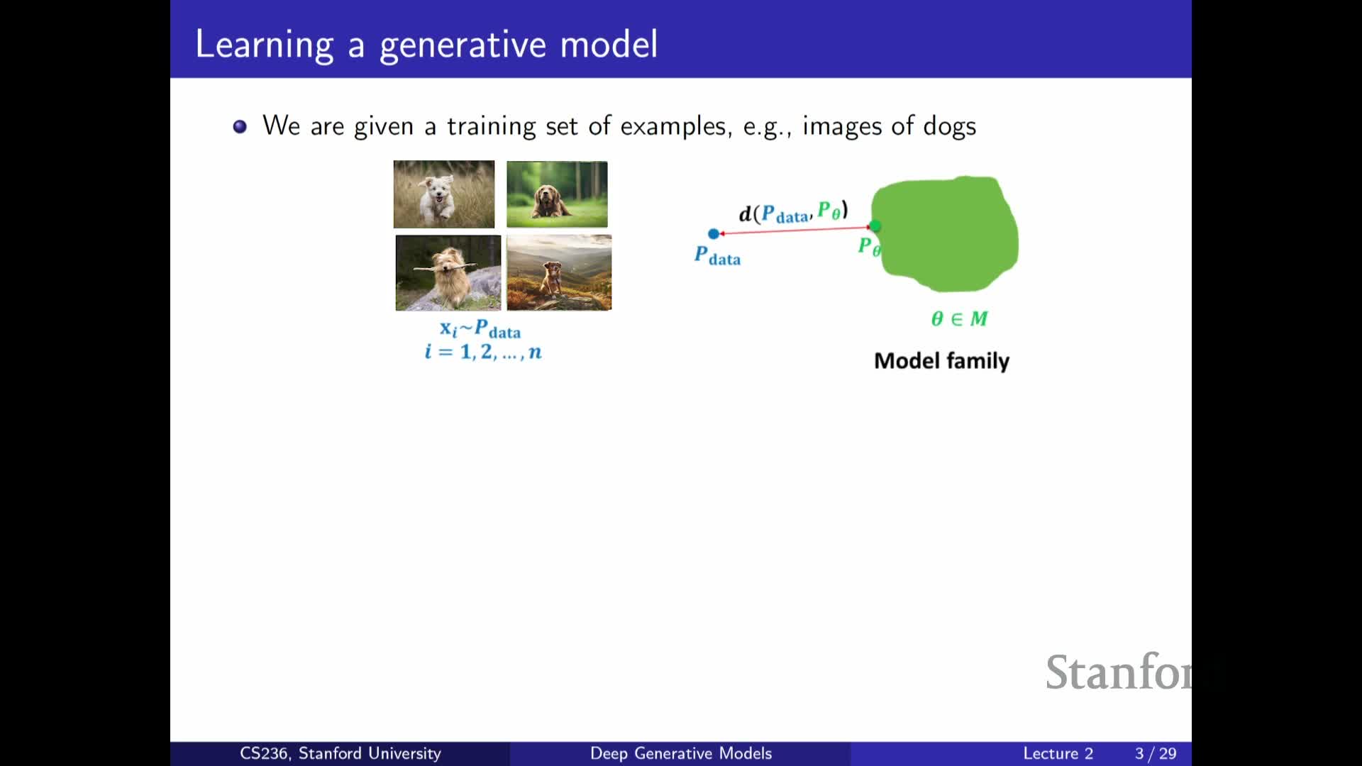
Describes the three fundamental components of generative modeling and how they interact:
-
Model family {P_theta} — a parameterized set of probability distributions that encodes representational assumptions.
-
Distance / loss — a metric that determines which discrepancies between distributions matter for the application.
-
Optimization procedure — the algorithm that projects P_data onto the model family by minimizing the chosen loss.
- The model family controls representational capacity and inductive biases.
- The loss dictates the kinds of errors we prioritize (e.g., mode coverage vs. sample fidelity).
- The optimizer governs what solutions are reachable in practice.
Together these components determine inductive biases, computational tractability, and the types of errors a generative model will make.
Applications of learned probability distributions
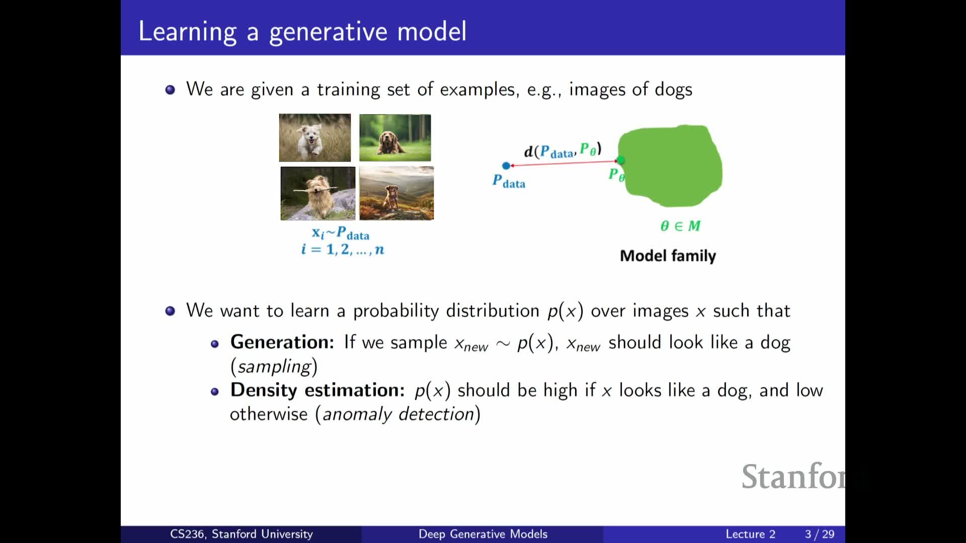
Enumerates practical uses for a learned approximation P_theta:
-
Sampling: generate new, synthetic data drawn from the modeled distribution.
-
Density estimation: assign likelihoods or scores to inputs under the model.
-
Anomaly detection: flag low-likelihood events as outliers.
-
Unsupervised feature discovery: extract latent structure or representations useful for downstream tasks.
A learned density gives a principled measure of how typical an input is under the data manifold, enabling additional tasks such as:
-
Imputation, controllable generation, semi-supervised learning, and discovery of axes of variation in the dataset.
These capabilities show why modeling the full distribution is valuable beyond pure classification objectives.
Representing probability distributions and the curse of dimensionality
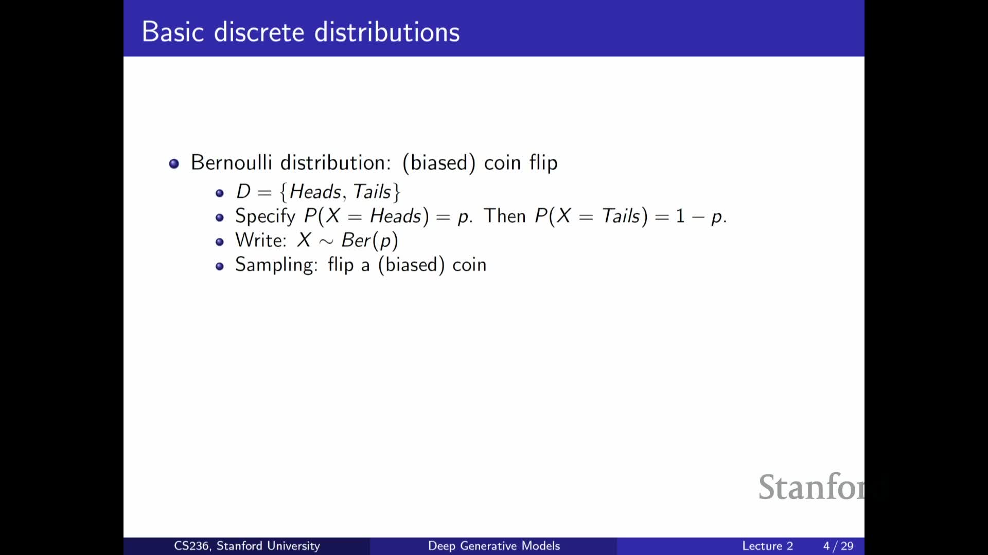
Introduces the core representational challenge: probability distributions over high-dimensional spaces are intractable to represent naively because the number of possible outcomes grows exponentially with dimensionality.
- Contrast trivial low-dimensional cases (e.g., Bernoulli, categorical) with high-dimensional structured objects (images, text).
- A direct tabular representation of the joint becomes impossible for realistic data: storage and estimation blow up exponentially.
This motivates the need for structural assumptions or compact parameterizations to obtain tractable models.
Discrete pixel modeling and combinatorial explosion in color spaces
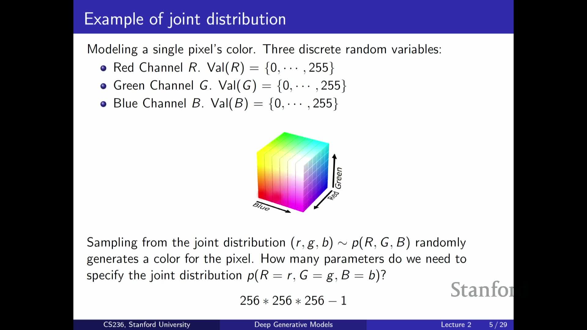
Explains how modeling pixel-level color distributions leads to combinatorial growth:
- With discrete RGB channels of 256 levels each, a single pixel can take 256^3 possible colors.
- A full joint over many pixels quickly becomes astronomically large, since a fully general joint requires specifying a probability for every discrete configuration.
Therefore, practical modeling requires structured factorizations or function-based parameterizations (e.g., neural networks) to compress representation and avoid the parameter explosion inherent in naive approaches.
Binary image example and the exponential state space 2^n
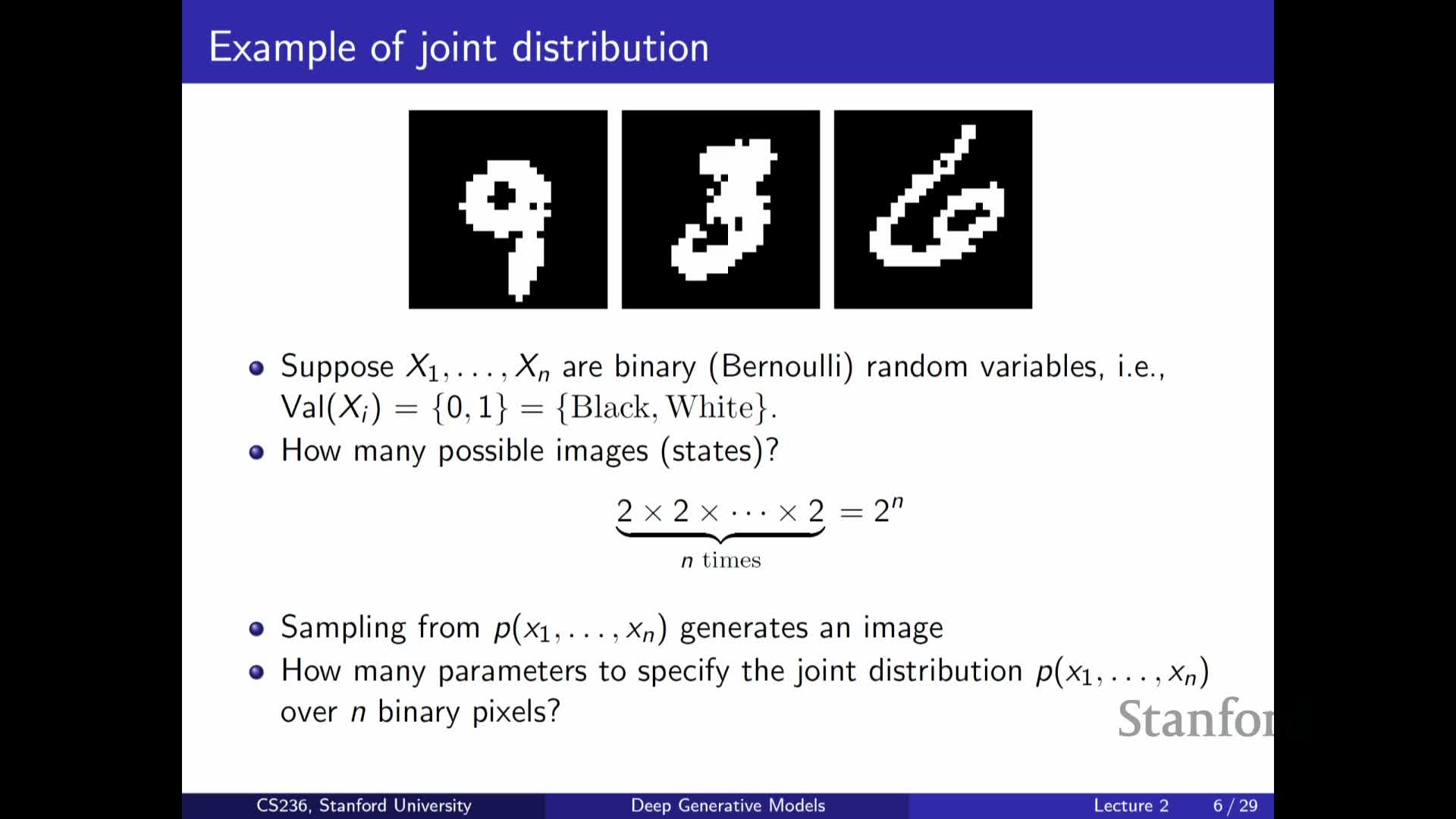
Illustrates the discrete-state explosion using black-and-white images:
- Model an image as n binary pixels ⇒ there are 2^n possible images.
- Even modest-resolution images produce an intractably large state space, so storing or learning a full table of probabilities is impossible in practice.
This forces us to adopt further assumptions—such as independence, conditional independence, or functional approximations—that dramatically reduce parameter count.
Assuming independence to reduce parameters and its limitations
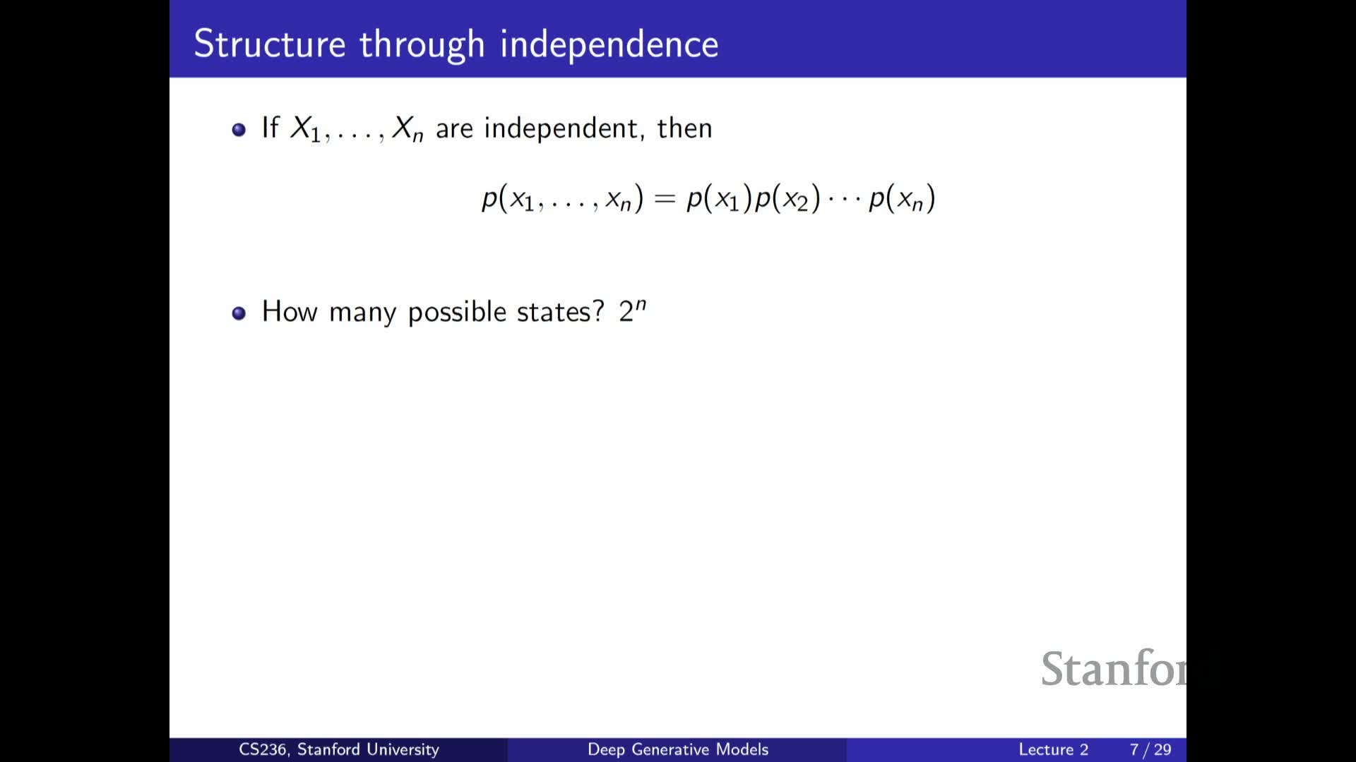
Describes the extreme approximation of modeling all pixels (or features) as independent:
- The joint becomes a product of marginals, reducing parameters from exponential to linear in the number of variables.
- Representation and learning become trivial under this assumption.
However, independence is typically far too strong for real-world data, which exhibit rich dependencies across dimensions, so samples from an independence model fail to capture coherent structure in images or text.
This trade-off exemplifies the tension between tractability and fidelity in model design.
Chain rule (autoregressive factorization) for joint distributions
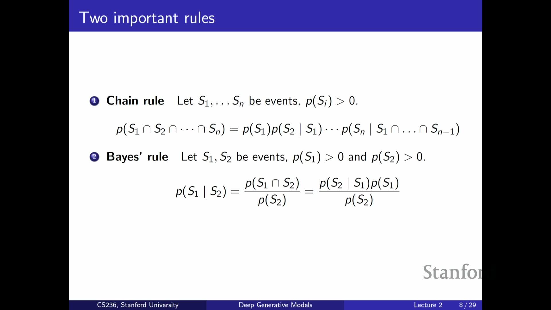
Presents the chain rule of probability as a fully general factorization:
-
Any joint can be written as P(x1) P(x2 x1) P(x3 x1,x2) … .
- This factorization underlies autoregressive models, enabling sequential sampling and likelihood evaluation by modeling each conditional in turn.
While the chain rule gives a principled decomposition of a complex joint into conditional factors, without further assumptions the conditionals themselves can still be intractably high-dimensional.
Parameter explosion in naive autoregressive models and Markov assumptions
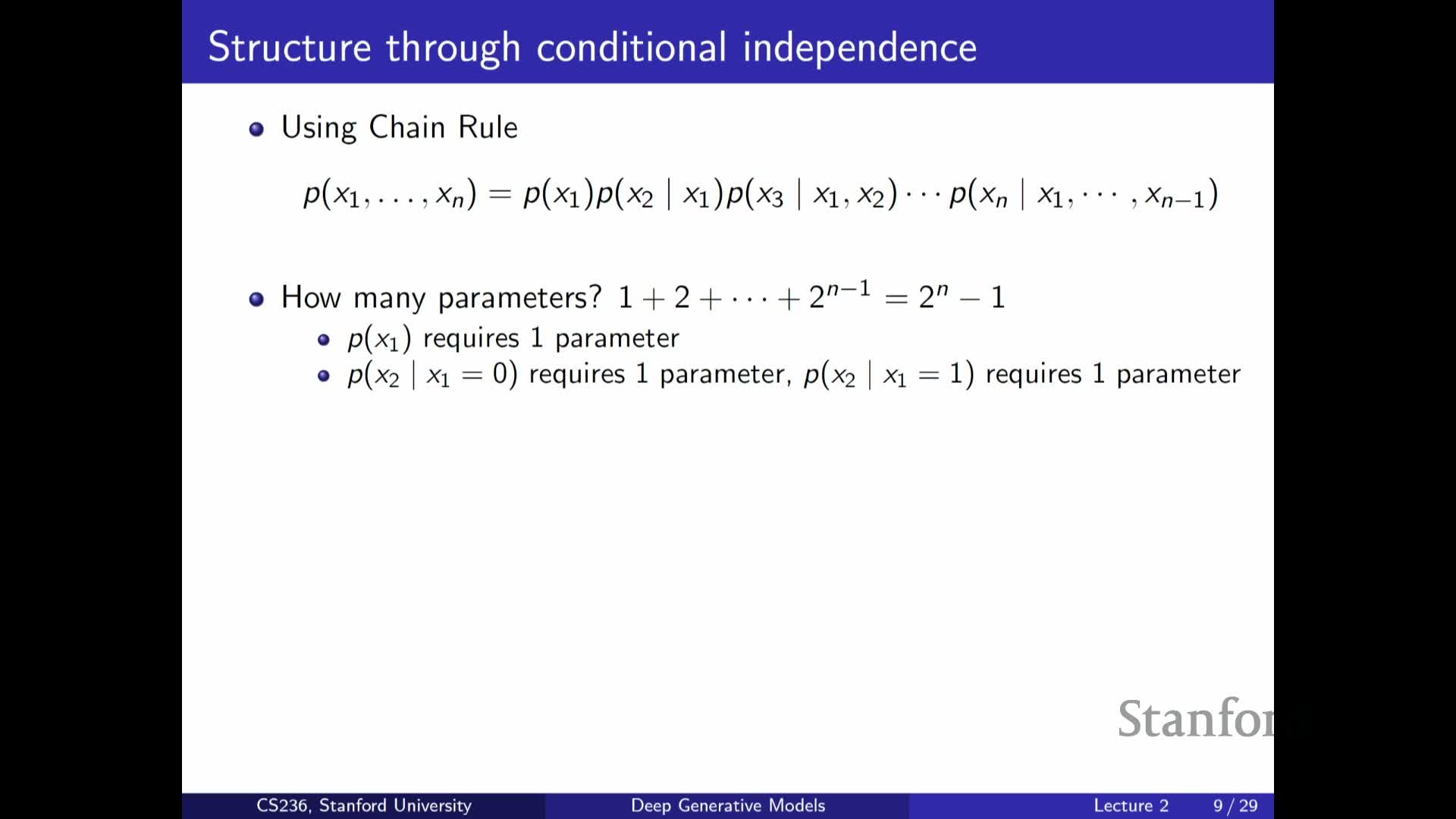
Analyzes parameter count for an unrestricted autoregressive factorization and how to make it tractable:
- An unrestricted factorization remains exponential because each conditional may require parameters for every configuration of its parents.
- Introducing Markov or limited-history conditional-independence assumptions (e.g., depend only on the previous k variables) reduces parameters from exponential to polynomial or linear in sequence length.
These conditional-independence simplifications trade expressive power for tractability and form the basis of practical autoregressive and sequence models.
Bayesian networks (directed graphical models) as structured factorization
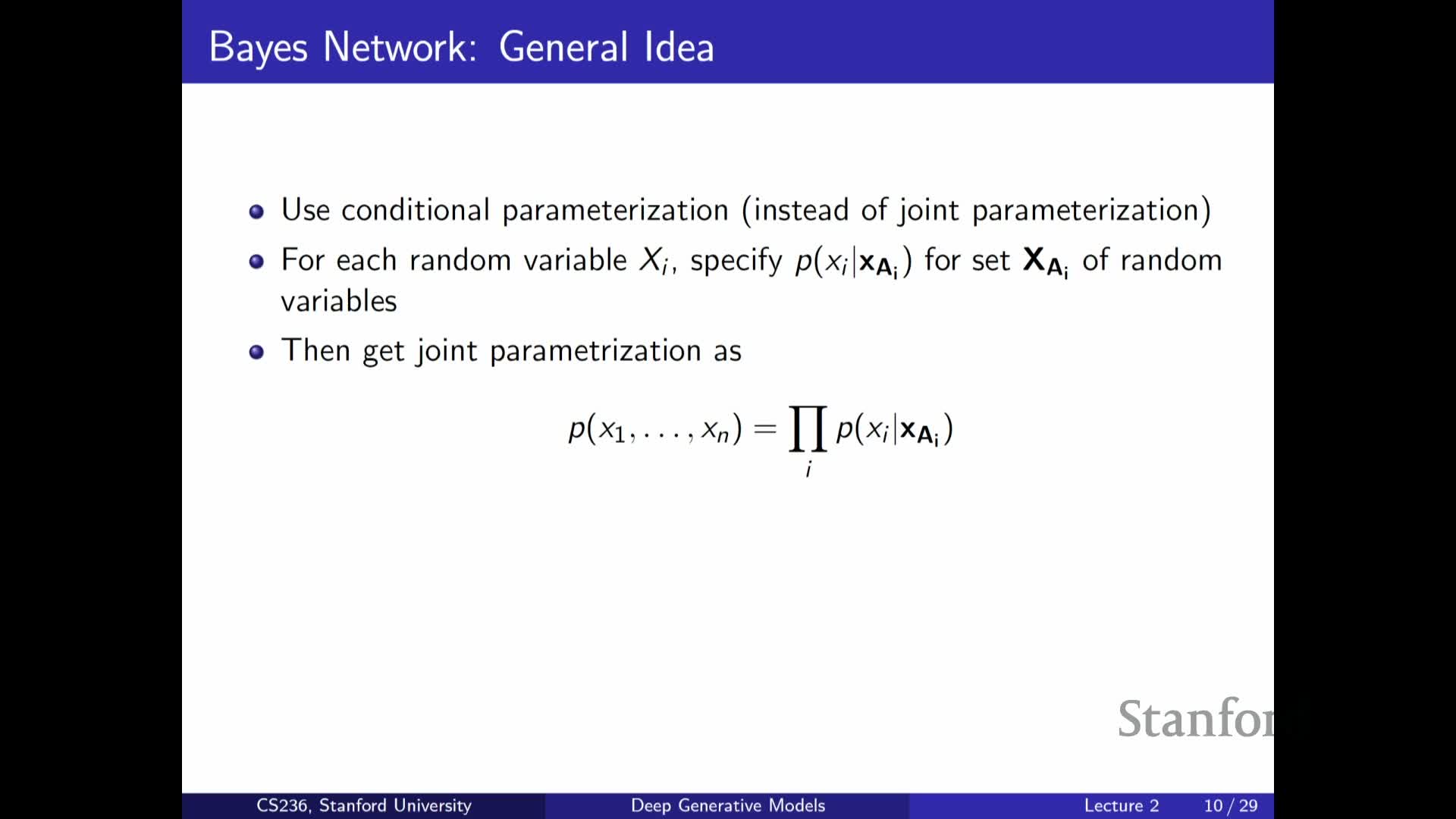
Defines Bayesian networks as directed acyclic graphs (DAGs) that encode a factorization of a joint distribution into local conditionals:
- Each node depends only on its parents in the graph.
- A Bayesian network is specified by a graph structure and a set of conditional probability tables or parameterized conditionals.
- A topological ordering plus the chain rule guarantees that the product of the local conditionals yields a valid joint distribution.
The graph structure encodes conditional independencies that can yield large representational savings when dependencies are local and parent sets are small.
Example Bayesian network: modeling exam difficulty, intelligence, grades
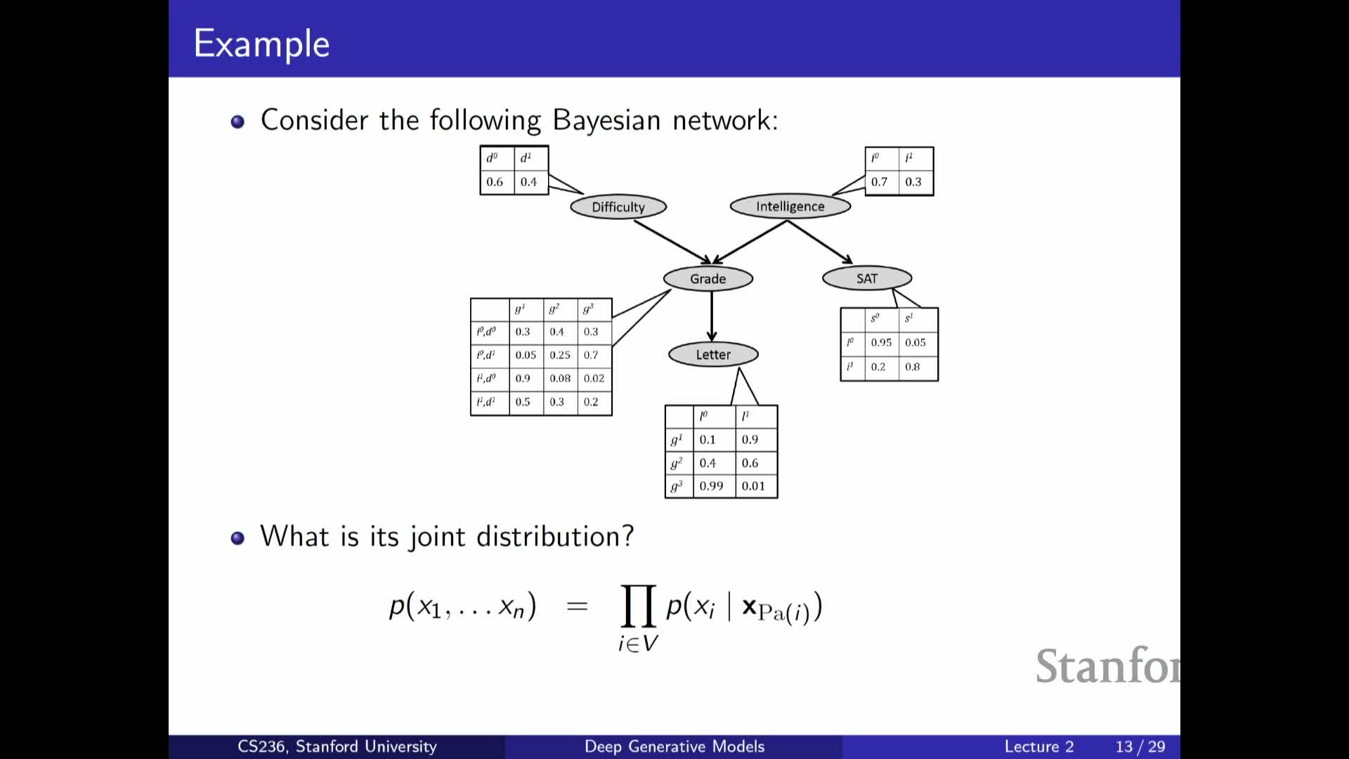
Presents a concrete Bayesian network example (exam difficulty, student intelligence, grades, SAT score):
- The joint factorizes into local conditionals according to the DAG (some nodes have no parents → marginals; others depend on a subset of variables).
- You only specify small conditional tables for each node instead of a full joint, reducing parameter complexity.
The example clarifies how domain assumptions translate into graph structure and how those assumptions simplify learning and inference.
Using graphical models versus neural networks for conditional structure
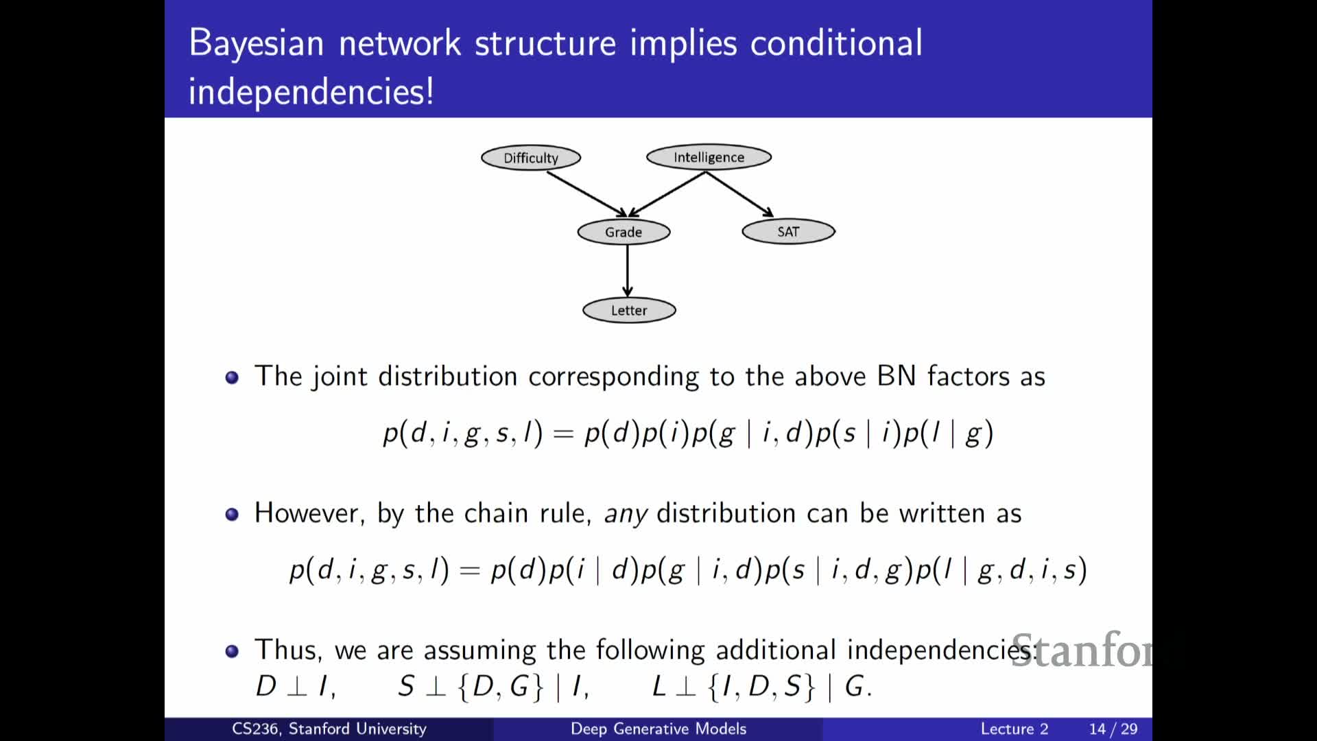
Summarizes the role of graphical models and motivates a shift to neural parameterizations:
-
Graphical models (Bayesian networks) are a principled tool to factorize and simplify joints via conditional independence.
- This lecture favors a softer approach: use neural networks to parameterize conditionals.
Neural conditionals relax strict independence assumptions and scale better to high-dimensional inputs, while retaining a graphical-model flavor by composing local conditionals into a global generative process—preparing the transition from classical PGMs to deep generative models.
Generative modeling applied to discriminative tasks: the Naive Bayes classifier

Describes Naive Bayes as a simple generative classifier:
-
It models the joint P(X, Y) by assuming conditional independence of features given the label, then uses Bayes’ rule to compute **P(Y X)** at prediction time.
-
Parameter estimation reduces to counting or estimating P(Y) and **P(X_i Y)** for each feature, which is tractable.
| Despite violated independence assumptions, Naive Bayes is often effective in practice and highlights the generative approach of modeling features explicitly, contrasting with purely discriminative methods that model **P(Y | X)** directly. |
Discriminative versus generative factorization and practical trade-offs
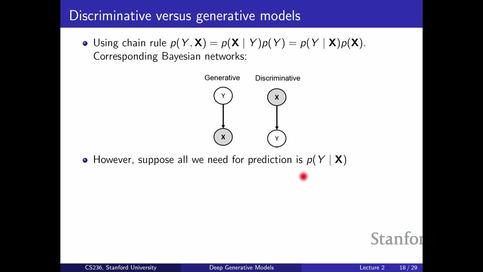
Compares discriminative and generative modeling approaches:
-
Discriminative models: directly model **P(Y X)** (or a predictive function), focusing only on the predictive task and often being more efficient when prediction is the sole goal.
-
Generative models: model the full joint P(X, Y) (e.g., **P(Y) P(X Y)) or other factorizations, supporting broader tasks such as **sampling, imputation, and density estimation.
Both approaches face exponential complexity when inputs are high-dimensional, so both require simplifying assumptions or parametric function classes to be practical.
Logistic regression as a functional parametrization of P(Y|X)
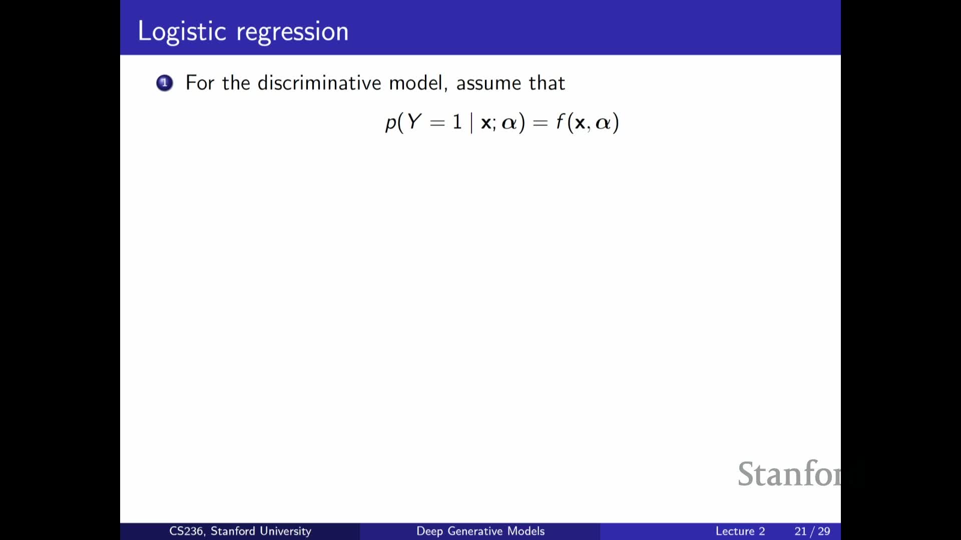
Explains how discriminative models avoid a tabular representation by assuming a functional form for P(Y | X):
-
Logistic regression is the canonical example: map a linear combination of features through a sigmoid to produce a probability in [0,1].
- This replaces an intractable lookup table with a low-parameter function f_alpha(X) that generalizes across feature vectors and can be trained from labeled data.
Logistic regression illustrates how imposing a simple functional form makes learning feasible while trading off representational capacity for parsimony and statistical efficiency.
Neural networks as richer functional parameterizations and deep autoregressive models
Describes how neural networks generalize logistic regression to richer function classes:
- Neural nets compute nonlinear features of X (layers like A X + b followed by activations and additional layers) before mapping to probabilities.
-
This provides far greater representational capacity for **P(Y X)** or for conditional factors in chain-rule factorizations.
| In generative modeling, this capacity underpins deep autoregressive models, where neural networks parameterize each conditional **P(x_t | x_<t). Scaling to long sequences requires **weight tying and careful architectural design. |
Design choices for deep generative models: factorization, parameter tying, and assumptions
Summarizes the core design levers for deep generative models:
- Choose a factorization (chain rule, BN structure, latent-variable model).
- Decide how to simplify or parameterize conditionals (conditional independence, parametric functions, neural networks).
- Determine parameter tying / shared architectures to enable scalable learning across positions or time steps.
Every choice trades expressivity, statistical efficiency, and computational tractability. Common successful patterns replace explicit independence with learned neural conditionals that are tied across positions or conditioned on latent variables.
Continuous variables, probability density functions, and latent-variable generative models (mixtures and VAEs)

Extends discrete concepts to continuous domains and introduces latent-variable generative patterns:
- Replace probability mass functions with probability density functions and assume parameterized functional forms (e.g., Gaussian, uniform) for tractability.
-
Bayesian-network-style factorizations naturally produce mixture models (e.g., a discrete latent Z chooses a cluster, then **X Z** is Gaussian).
-
Latent-variable models combine a simple prior P(Z) with neural-network-parameterized conditionals **P(X Z; theta)** to obtain expressive families.
This is the generative-process pattern used in variational autoencoders: sample latent Z from a simple prior, compute conditional parameters via neural networks, then sample X from the resulting conditional density.
Enjoy Reading This Article?
Here are some more articles you might like to read next: