Stanford CS236- Deep Generative Models I 2023 I Lecture 3 - Autoregressive Models
- Course introduction and scope
- Generative modeling pipeline and training objective
- Use cases for explicit probability models
- Chain rule factorization as a universal representation
- Neural approximation of conditionals
- Conditional prediction as a classification/regression building block
- Modeling images as autoregressive sequences (binarized MNIST example)
- Choice of ordering and simple per-pixel models (fully visible sigmoid belief network)
- Evaluating joint likelihoods and sequential sampling
- Limitations of per-step logistic models and move to neural autoregressive density estimation
- Weight tying and shared-parameter autoregressive networks
- Model outputs for discrete, categorical, and continuous variables
- Relation between autoregressive decoders and autoencoders and the VAE remedy
- Masked neural networks to implement autoregressive factorization in a single network
- Recurrent neural networks as compact autoregressive models for sequences
Course introduction and scope

Autoregressive models are presented as a primary family of deep generative models—they are the fundamental technology behind many large language models and related contemporary systems.
Generative modeling pipeline and training objective
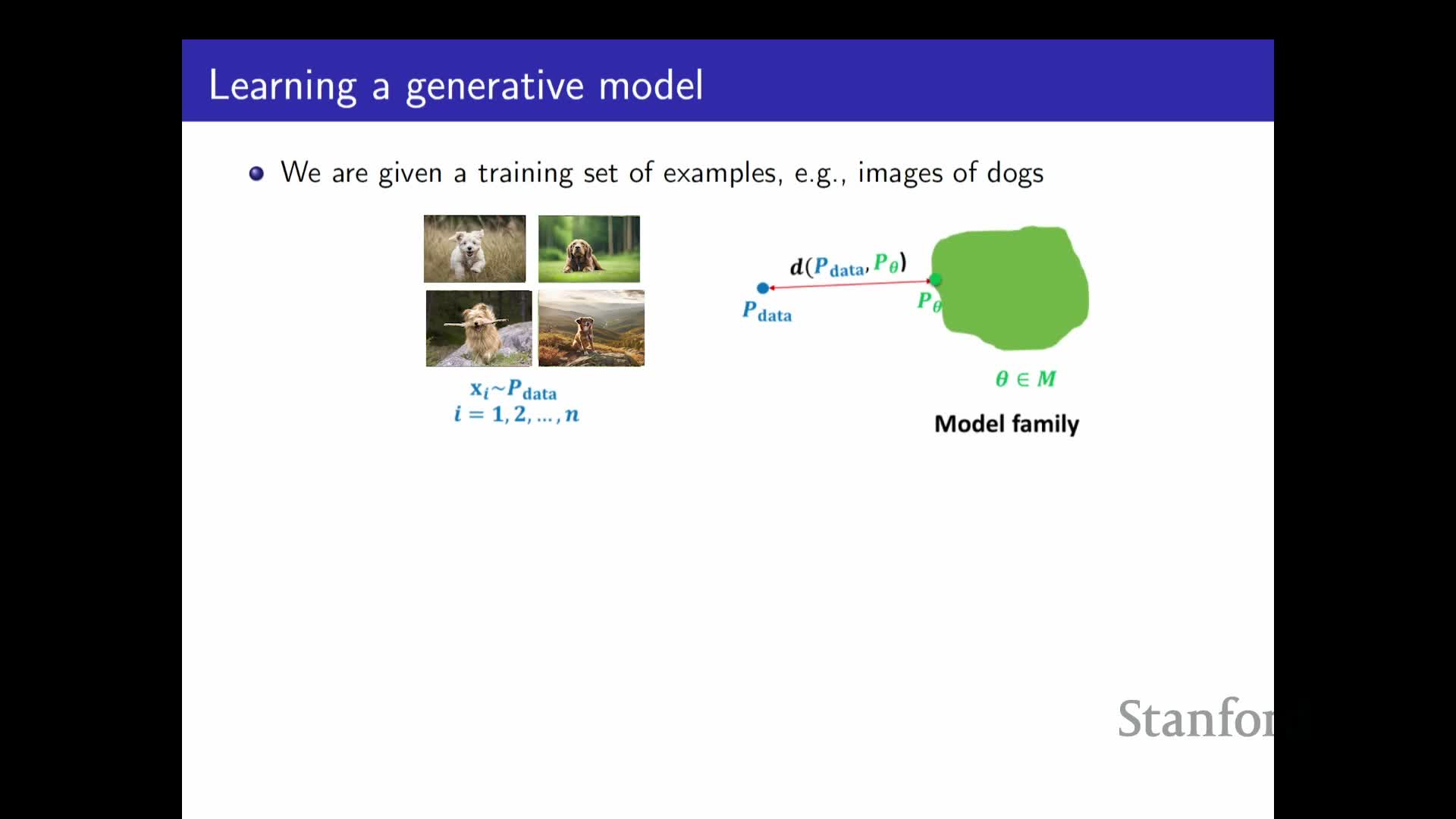
A generative modeling pipeline requires several core ingredients:
-
IID samples drawn from an unknown data distribution (we only have samples, not the density).
- A parameterized model family defined over the data domain (parameters denoted θ).
- A divergence or similarity criterion to measure closeness between the model and the data distribution.
Training typically proceeds by adjusting θ, most commonly via maximum likelihood, so that the model distribution approximates the data distribution using only observed samples.
Use cases for explicit probability models
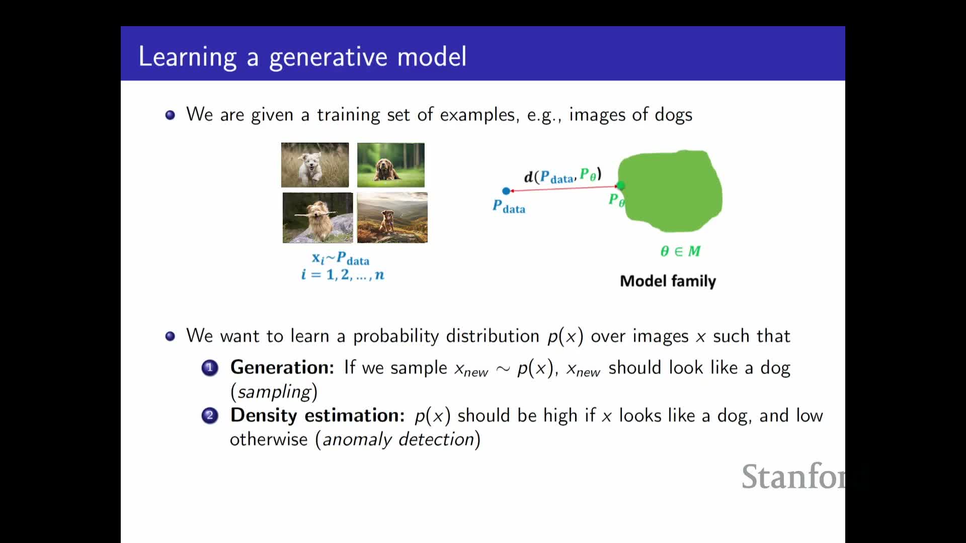
Explicitly modeling probabilities enables several key capabilities:
-
Sampling — generate new data by drawing from the modeled distribution.
-
Maximum-likelihood training — evaluate model probabilities to fit parameters to data.
-
Anomaly detection — identify low-likelihood inputs as potential outliers.
-
Unsupervised representation learning — capturing structure in the data can produce useful features for downstream supervised tasks.
Chain rule factorization as a universal representation
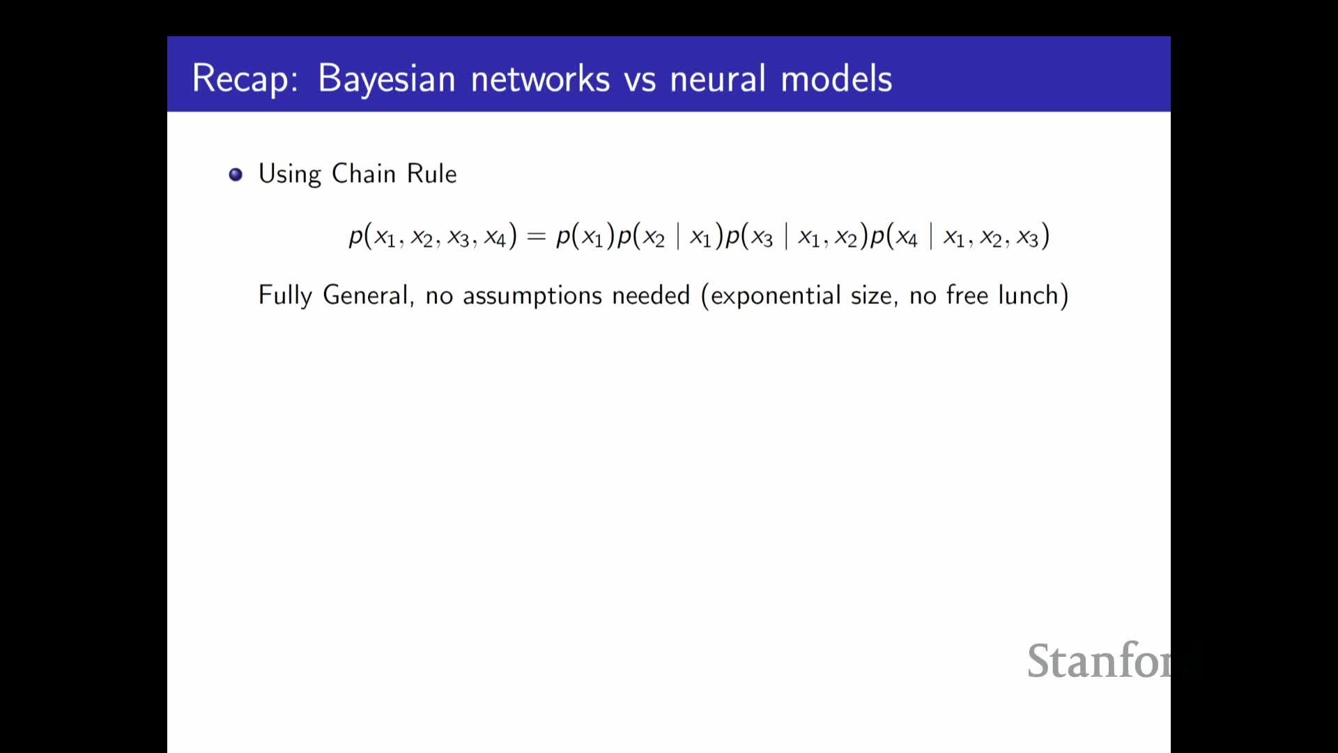
Chain-rule factorization: any joint distribution over multiple variables can be written exactly as a product of conditional distributions in an arbitrary ordering:
-
p(x1, …, xN) = p(x1) p(x2 x1) p(x3 x1,x2) … p(xN x1,…,xN-1).
- The choice of ordering affects modeling convenience and efficiency, but the factorization itself is universally valid.
- This factorization reduces a high-dimensional density estimation problem to a sequence of conditional prediction problems.
Neural approximation of conditionals
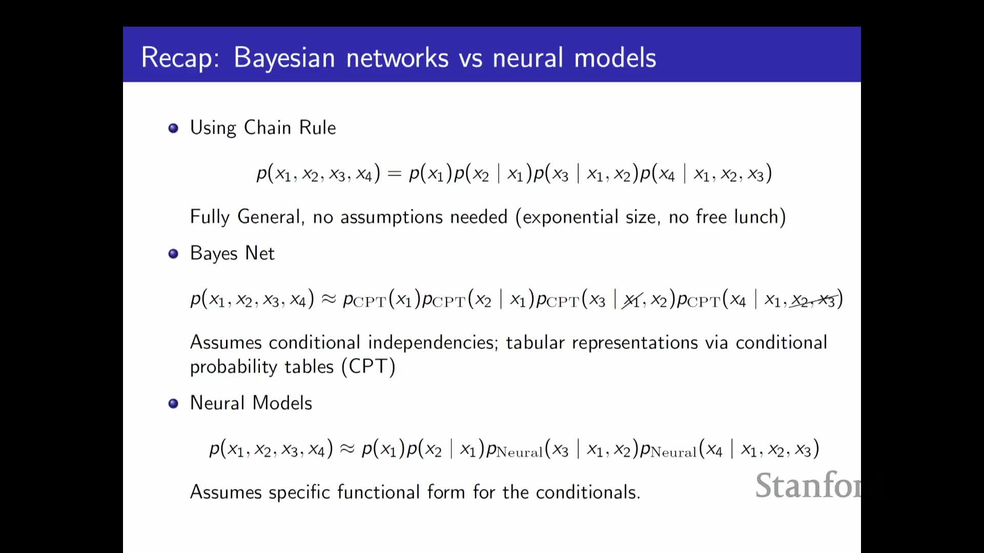
Autoregressive modeling uses neural networks to approximate the chain-rule conditionals:
- Neural parameterizations replace tabular conditional probability tables, making estimation tractable for complex dependencies.
- This works provided the chosen network architecture is sufficiently expressive to approximate the true conditional functions.
Conditional prediction as a classification/regression building block
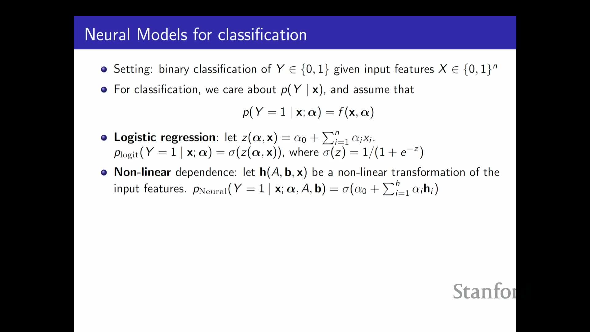
The basic building block is predicting a single variable conditioned on many inputs—analogous to classification or regression:
- For simple linear dependencies, one can use logistic regression (binary) or linear regressors.
- For nonlinear dependencies, use deep networks to capture complex conditional structure.
- Stacking these conditional predictors according to a chosen ordering yields a full autoregressive generative model.
Modeling images as autoregressive sequences (binarized MNIST example)
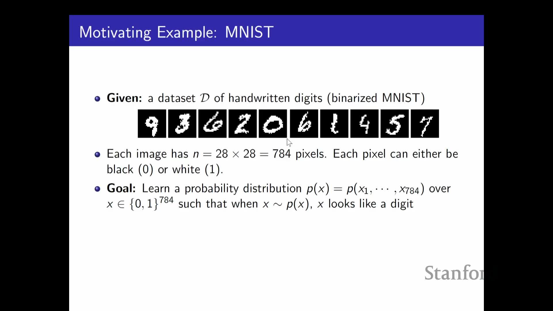
An image with discrete pixels can be treated as a sequence of random variables:
- Example: binarized MNIST (28 × 28) yields 784 binary variables.
- A joint distribution over images is specified by choosing an ordering of the pixels and modeling each pixel’s conditional distribution given previous pixels.
- This reduces image generation to a sequence of tractable, single-variable prediction problems.
Choice of ordering and simple per-pixel models (fully visible sigmoid belief network)
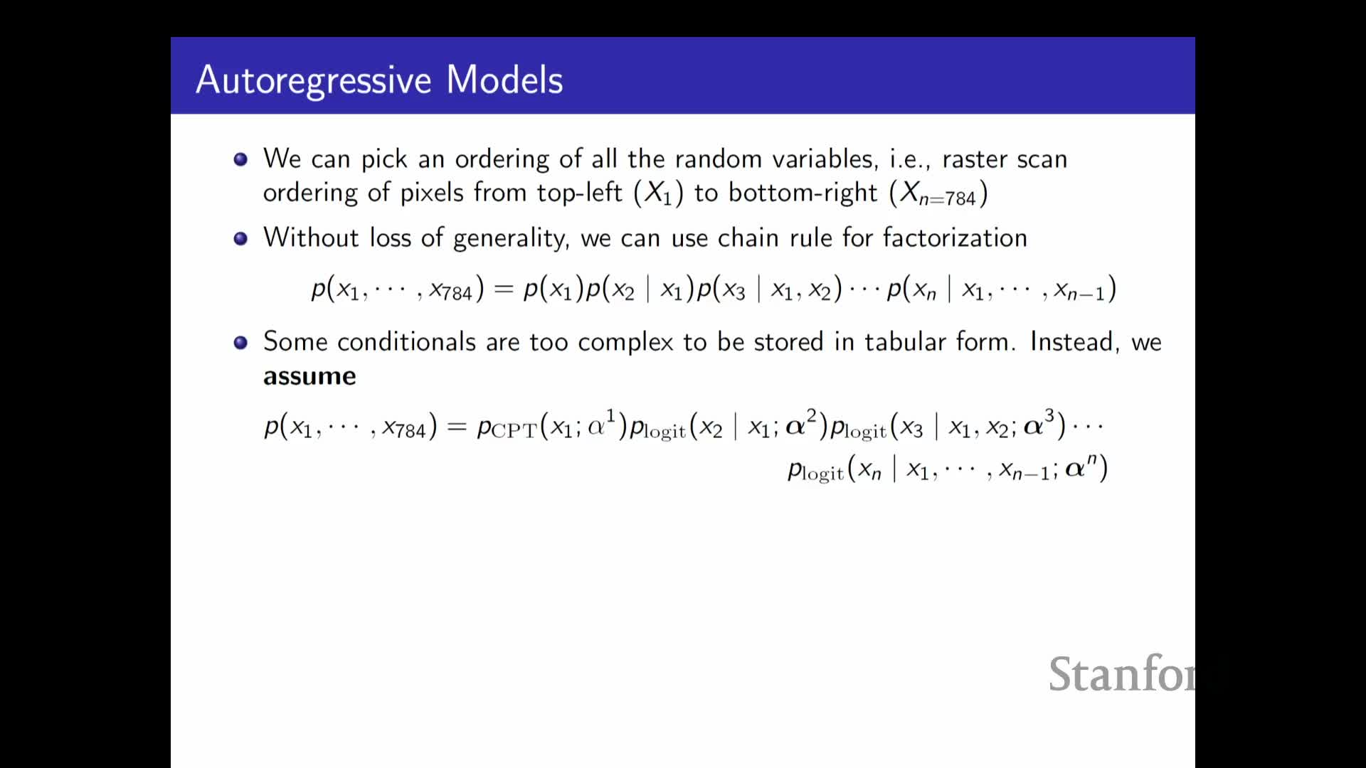
Any ordering (for example raster scan) can be used to apply the chain rule, but the induced conditional structure affects ease of prediction:
- A naive approach uses independent logistic regressions per conditional, known as the fully visible sigmoid belief network.
- This naive scheme scales poorly in parameters and often lacks the expressivity needed to capture complex pixel dependencies.
Evaluating joint likelihoods and sequential sampling
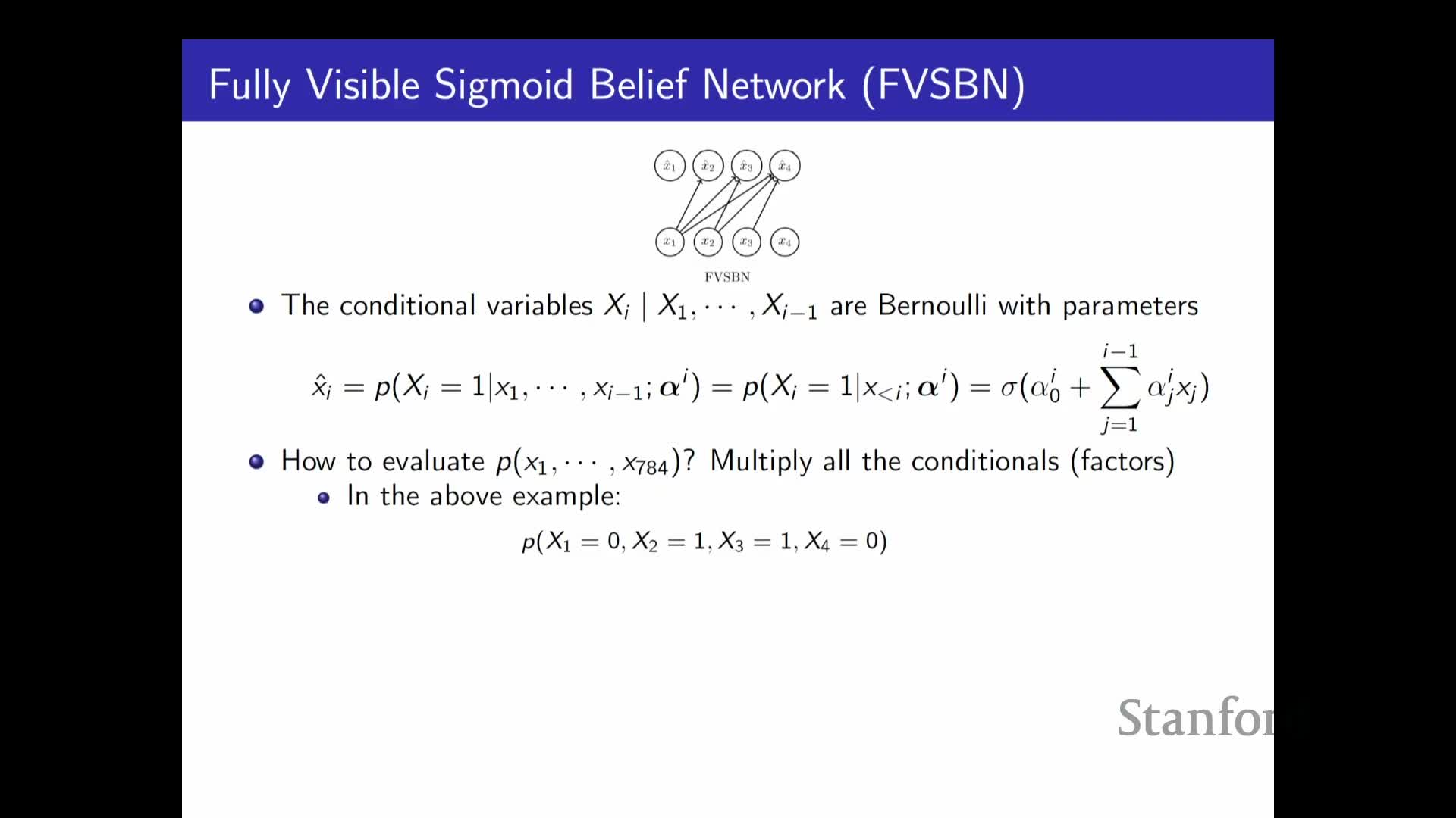
Computing likelihoods and sampling under an autoregressive model:
-
Joint likelihoods are computed by multiplying the predicted conditional probabilities according to the chain-rule factorization—i.e., product of per-step conditionals.
-
Sampling is done sequentially: sample the first variable from its marginal, then each subsequent variable from its conditional given previously sampled variables.
- This yields exact ancestral sampling, but it requires sequential computation at generation and evaluation time.
Limitations of per-step logistic models and move to neural autoregressive density estimation
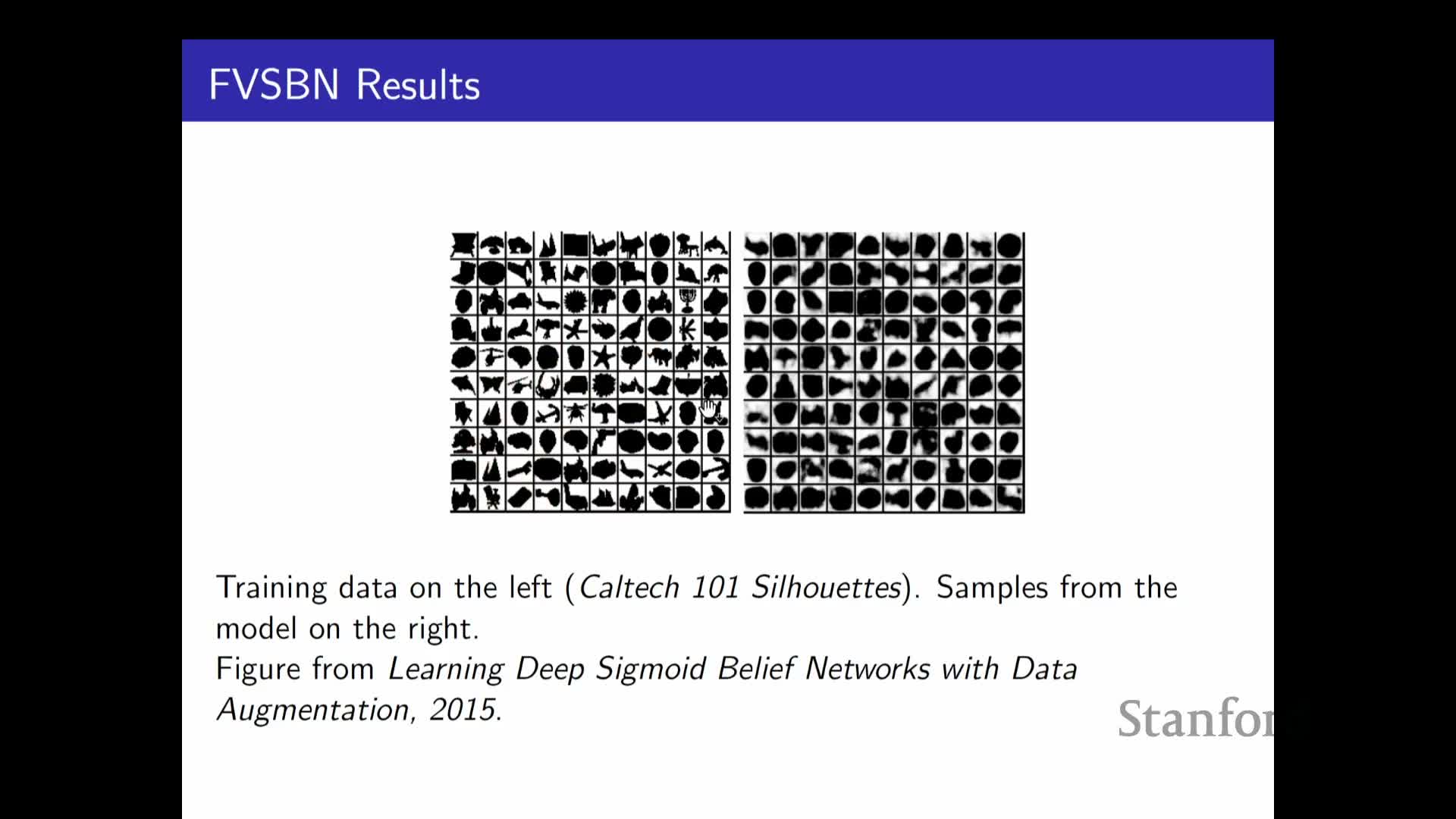
Simple logistic-per-pixel models typically produce low-quality samples because they cannot represent complex conditionals.
- Replacing per-step logistic regressions with neural networks (single-layer or deeper) yields neural autoregressive density estimators.
- These neural parameterizations increase conditional expressivity and substantially improve sample quality.
Weight tying and shared-parameter autoregressive networks

Tying weights across per-step predictors is an important efficiency and generalization strategy:
- Use a single shared parameter matrix and select appropriate slices for each conditional.
- Benefits:
- Reduces parameter count from roughly quadratic to roughly linear in the number of variables.
- Enforces parameter sharing that can improve generalization.
- Enables reuse of intermediate computations to evaluate many conditionals more efficiently during training and likelihood computation.
- Reduces parameter count from roughly quadratic to roughly linear in the number of variables.
Model outputs for discrete, categorical, and continuous variables

Autoregressive predictors output the parameters of the appropriate conditional distribution depending on variable type:
- For multi-valued discrete variables: output a K-way categorical distribution via softmax over K logits.
- For continuous variables: output parameters of a continuous density (e.g., a Gaussian or a mixture of Gaussians).
- The network predicts means, variances, and mixture weights to represent multimodal conditional densities.
- The network predicts means, variances, and mixture weights to represent multimodal conditional densities.
Relation between autoregressive decoders and autoencoders and the VAE remedy
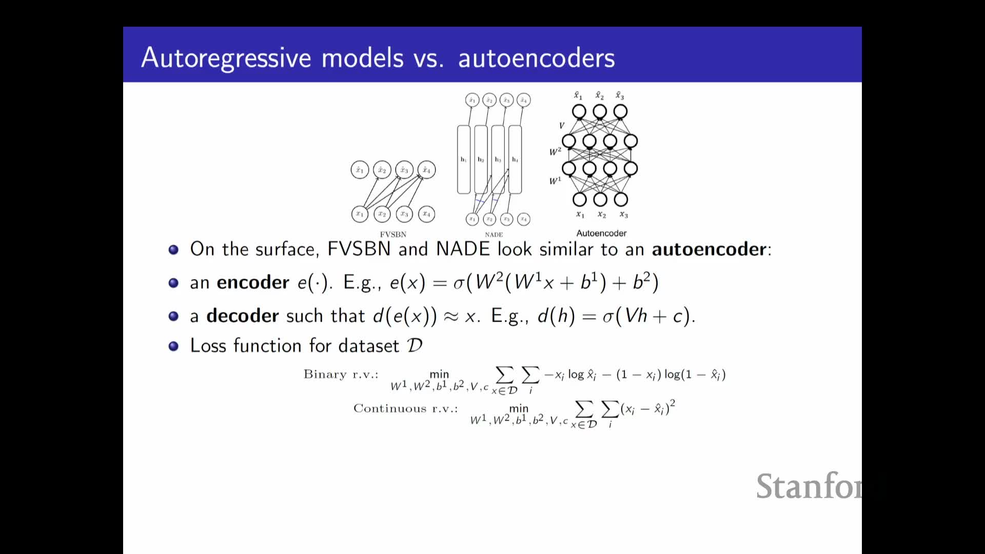
Relationship to autoencoders and VAEs:
- An autoregressive decoder resembles the decoder in an autoencoder computation graph.
- A vanilla autoencoder lacks a prescribed prior over latent inputs, so it does not provide a mechanism to sample new data directly.
- Imposing a prior on latents and training jointly (the variational autoencoder approach) enables sampling by drawing latents from the prior and feeding them to the decoder.
- By contrast, autoregressive models enforce a sequential structure that makes ancestral sampling possible without a separate latent prior.
Masked neural networks to implement autoregressive factorization in a single network
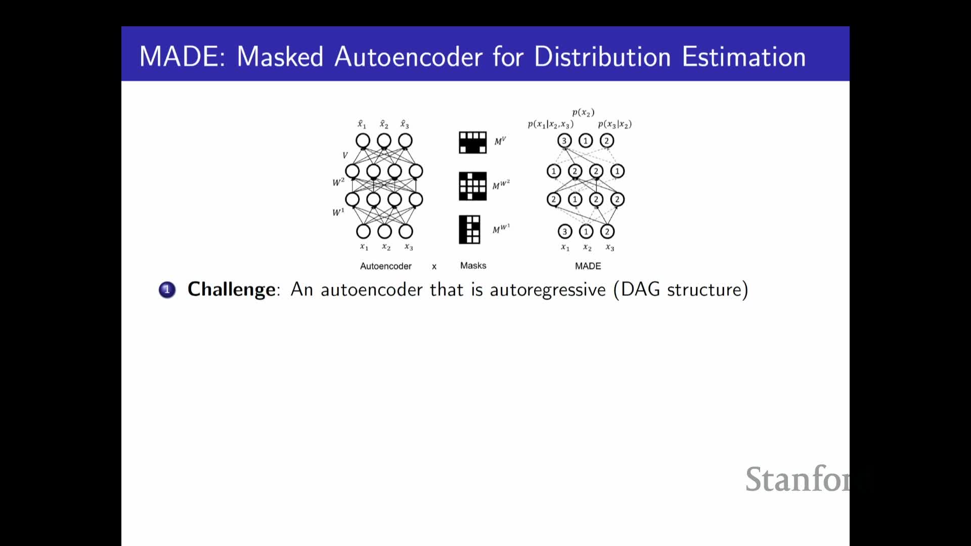
Implementing autoregressive factorization as a single feed-forward network via masking:
- Apply weight masks so each output unit depends only on allowed input indices (i.e., previous variables in the chosen ordering).
- This preserves the chain-rule invariant and prevents “cheating” by access to future variables.
- Benefits:
- A single forward pass can produce all conditional parameters during training.
- Efficient evaluation while ensuring each conditional only uses permitted inputs.
- A single forward pass can produce all conditional parameters during training.
Recurrent neural networks as compact autoregressive models for sequences
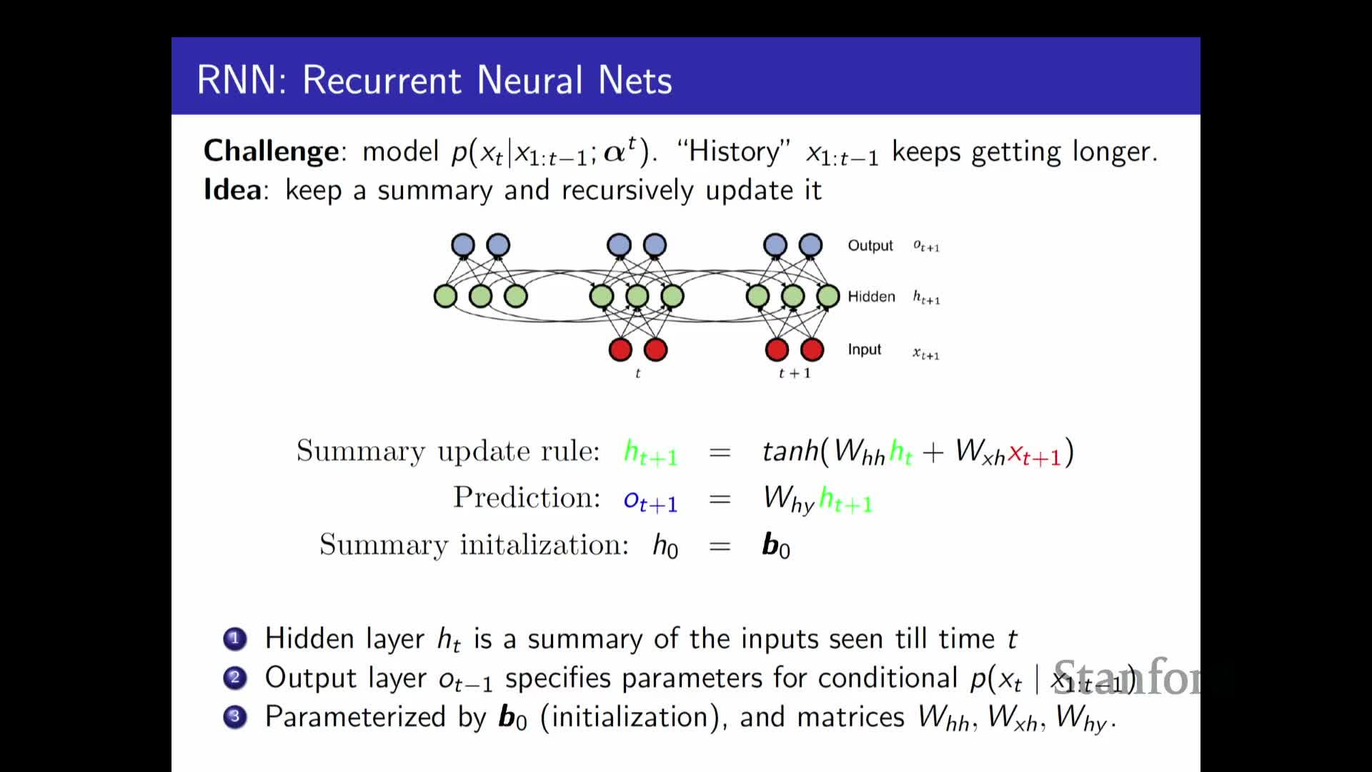
Recurrent neural networks (RNNs) implement autoregressive factorization using a recursive hidden-state update:
- The RNN summarizes past variables into a fixed-size hidden state via recurrent updates.
- That hidden state is then mapped to conditional distribution parameters for the next variable.
- Advantages:
- Parameter storage is constant with respect to sequence length.
- Can model arbitrarily long sequences in principle.
- Parameter storage is constant with respect to sequence length.
- Limitations:
- Generation and evaluation remain sequential operations.
- Learning can be challenging because the model must compress history into a single fixed-size state.
- Generation and evaluation remain sequential operations.
Enjoy Reading This Article?
Here are some more articles you might like to read next: