Stanford CS236- Deep Generative Models I 2023 I Lecture 4 - Maximum Likelihood Learning
- RNNs parameterize autoregressive models using a fixed-size recurrent state
- RNNs suffer from representational bottlenecks and training inefficiencies due to unrolled recursion
- Attention computes relevance between query and key vectors to form context-weighted predictions
- Self-attention and masking enable parallel, autoregressive Transformers that scale efficiently
- Autoregressive models can be applied to images by treating pixels (and channels) as sequence elements with masked dependencies
- Masked convolutions and attention on images enforce autoregressivity but introduce architectural trade-offs
- Choosing an ordering for non-sequential data is arbitrary and can be learned but often uses simple heuristics
- Transformer and convolutional autoregressive models can match or outperform RNNs in training efficiency while RNNs retain inference-time advantages
- Autoregressive likelihoods permit sample-based anomaly detection and can distinguish adversarially perturbed inputs
- Learning begins with defining objectives and the desiderata for model approximation; density estimation is a canonical target
- The Kullback–Leibler divergence quantifies distributional discrepancy and has an information-theoretic compression interpretation
- Minimizing forward KL between the data distribution and model reduces to maximizing expected log-likelihood under the data and yields maximum likelihood estimation
- The empirical average (Monte Carlo) approximates expectations and yields the practical MLE objective implemented as negative log-likelihood over the dataset
- Gradient-based optimization of autoregressive models uses backpropagation and stochastic minibatch estimates for scalability
- Generalization requires controlling model complexity via regularization, validation, and bias–variance trade-offs
RNNs parameterize autoregressive models using a fixed-size recurrent state
Recurrent neural networks (RNNs) implement autoregressive probabilistic models by maintaining a fixed-size hidden state that summarizes past observations and conditions the distribution over the next token or pixel.
- The hidden state is updated recurrently as new symbols are observed.
-
The state at time t parameterizes the conditional distribution **p(x_t x_1:t-1)**. - This parameterization yields a model family whose parameter count is independent of sequence length.
- It is applicable at token/character levels and to pixel-by-pixel image generation.
By casting next-step prediction as a sequence of per-step classification problems conditioned on the rolling state, RNNs provide a straightforward mechanism for sampling and likelihood computation via the chain rule.
RNNs suffer from representational bottlenecks and training inefficiencies due to unrolled recursion
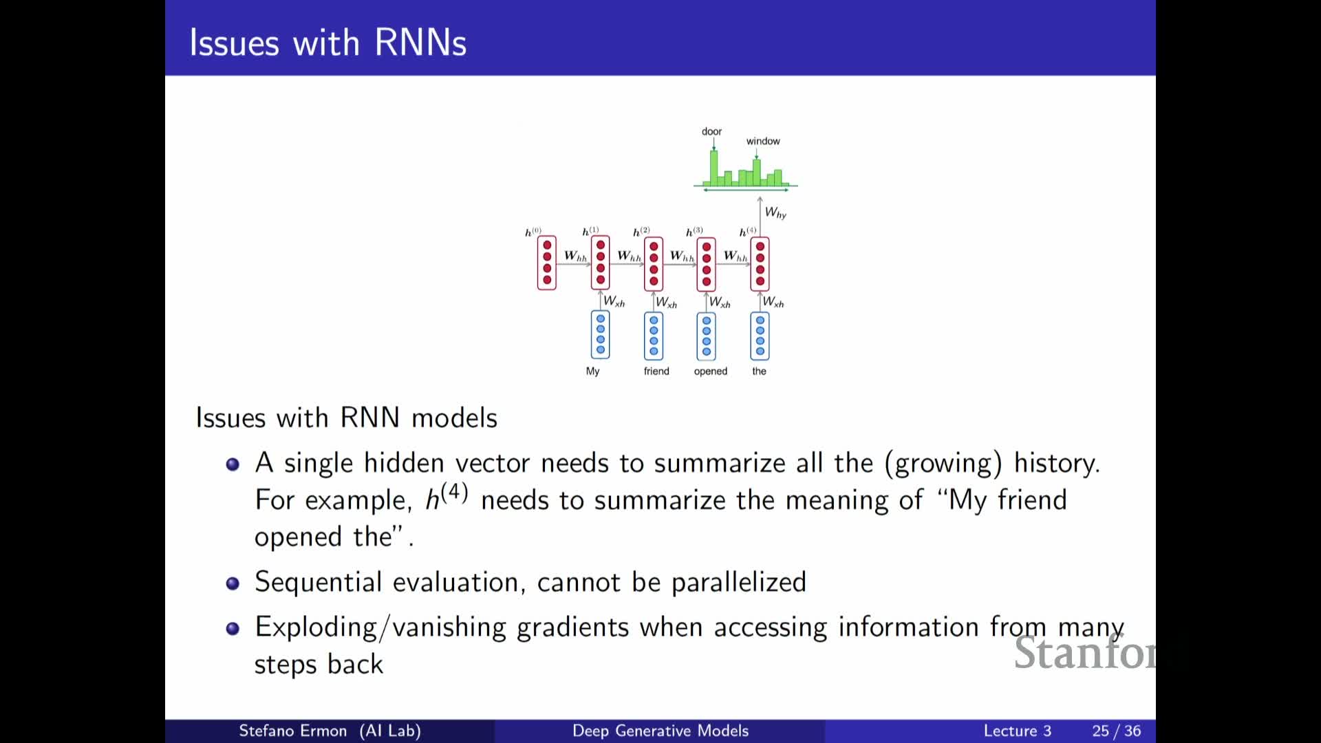
Using a single fixed-size hidden vector to summarize arbitrarily long context creates a representational bottleneck that can fail to capture long-range dependencies.
- Training requires unrolling the recurrent computation through time, which:
- Reduces parallelism across time steps,
- Increases wall-clock training time,
- Complicates optimization because gradients must propagate through many steps.
- Long-range dependencies thus exacerbate vanishing or exploding gradients, making RNNs slower and harder to train in practice despite their theoretical expressivity.
These practical limitations motivate alternative architectures that avoid sequential unrolling during training.
Attention computes relevance between query and key vectors to form context-weighted predictions
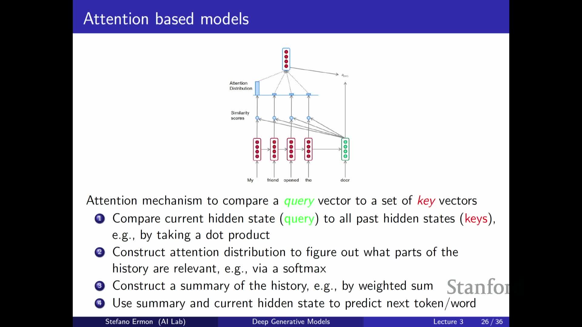
Attention mechanisms compute a relevance score between a query vector and a set of key vectors (commonly via a dot product), then convert those scores into a normalized attention distribution (typically with softmax).
- The resulting attention weights are used to form a weighted average of value vectors, producing a context vector that selectively aggregates information from the entire past sequence.
- The query–key–value formulation generalizes retrieval: the model can focus on specific past elements instead of compressing all history into a single hidden state.
- This selective access improves modeling of long-range and structured dependencies.
Self-attention and masking enable parallel, autoregressive Transformers that scale efficiently
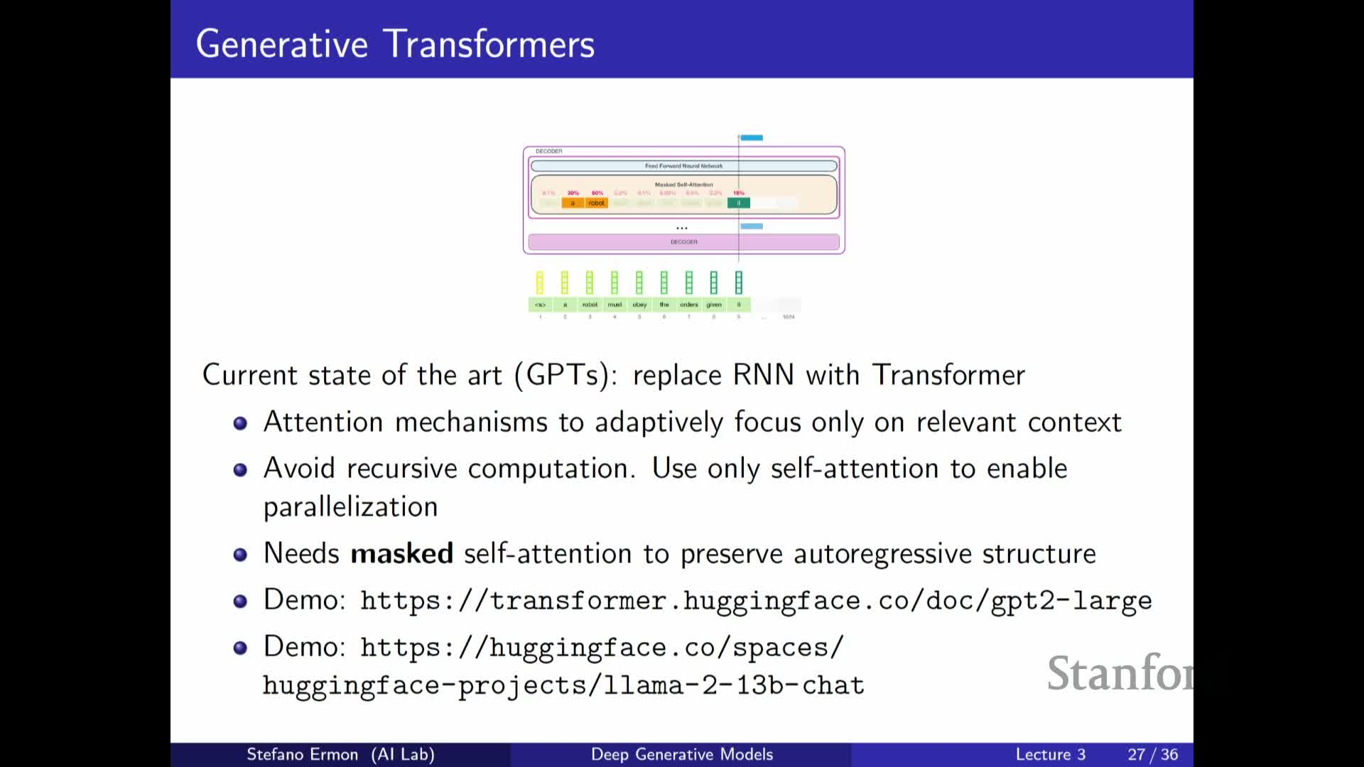
Self-attention stacks let each position attend to all previous positions and, with appropriate causal masking, enforce an autoregressive factorization while permitting highly parallel feed-forward computation across positions.
- Causal masking prevents attention to future tokens so the model remains autoregressive.
- Stacking multiple attention layers increases representational depth without temporal recursion.
- The approach yields:
- Massive GPU parallelism,
- Efficient loss evaluation across all positions,
- The scaling behavior behind state-of-the-art autoregressive language models (e.g., GPT variants).
Autoregressive models can be applied to images by treating pixels (and channels) as sequence elements with masked dependencies
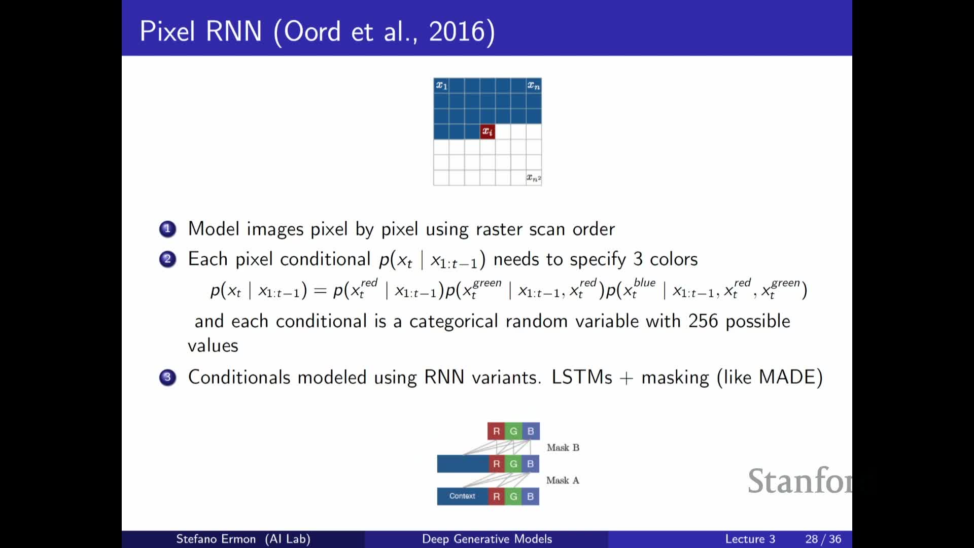
Images can be modeled autoregressively by linearizing pixels into a sequence (e.g., raster scan order) and defining a conditional distribution for each pixel given preceding pixels.
- For color images, channels (red, green, blue) are further factorized so that later channels condition on previously generated channels for the same pixel.
- Each conditional is a discrete or continuous distribution over pixel intensities and is parameterized by an RNN, CNN, or attention-based network with masking that enforces the chosen ordering.
-
Sampling and likelihood evaluation follow directly from the chain rule, but naive sequential evaluation is slow—hence masked convolutions or masked attention implementations are used to speed up training and generation.
Masked convolutions and attention on images enforce autoregressivity but introduce architectural trade-offs
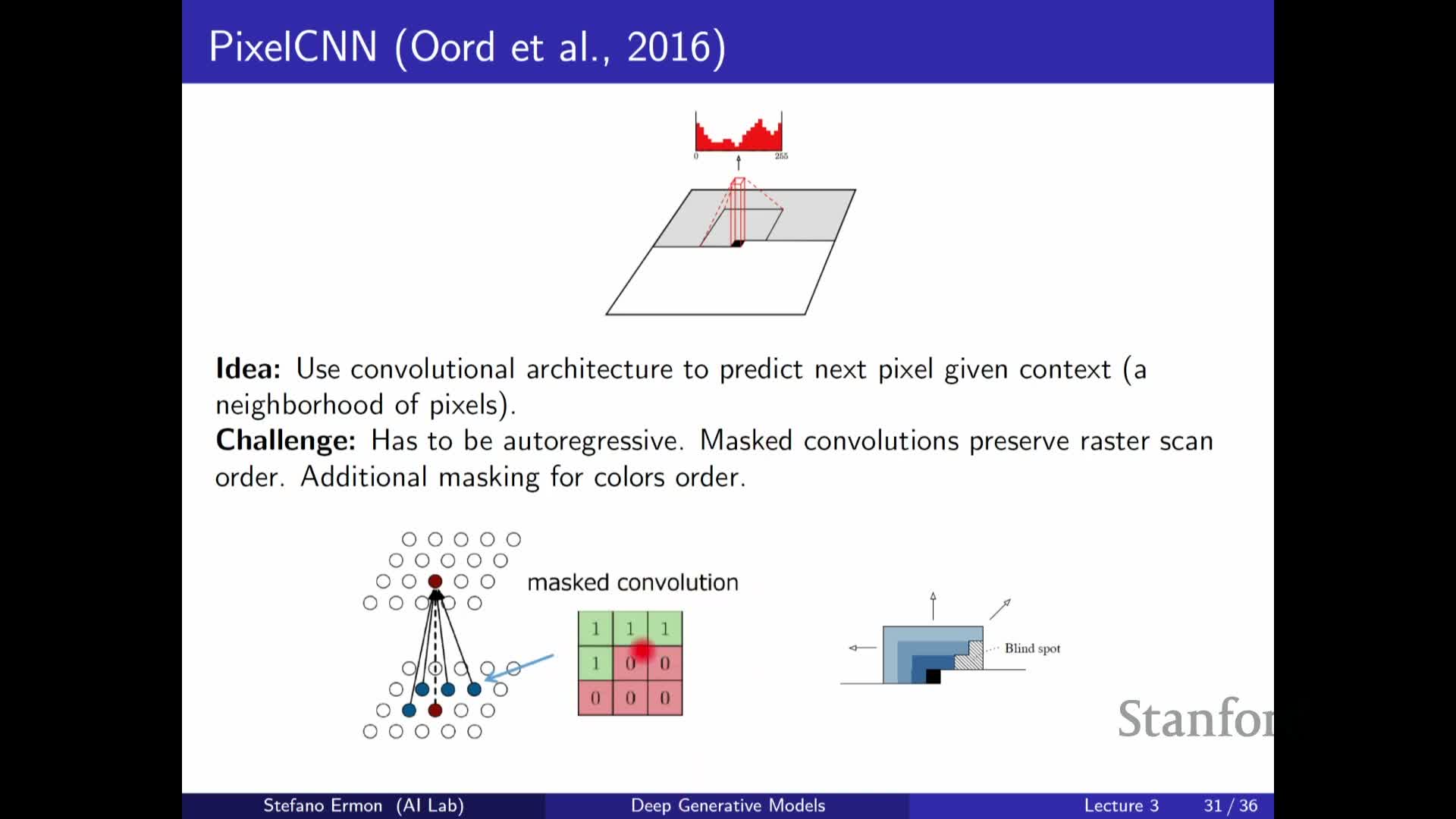
Convolutional architectures can be adapted to autoregressive image modeling by zeroing-out kernel entries or applying causal masks so predictions for a target pixel do not depend on future pixels.
- This enables efficient parallel matrix-multiplication implementations on modern hardware.
- However, masked convolutions can create receptive-field blind spots unless kernels and layer arrangements are designed carefully. Architectural tricks (e.g., staggered masks or mixed masks) are used to cover all relevant context.
-
Transformer-style masked self-attention can also be applied to images and has shown promise, although it can be computationally heavier than convolutional or diffusion-based approaches at large scale.
Choosing an ordering for non-sequential data is arbitrary and can be learned but often uses simple heuristics
For data without a canonical temporal ordering (like images), one must select an ordering to define an autoregressive factorization.
- Common choices include top-left-to-bottom-right raster order, but alternative or learned permutations can be explored.
- The chosen ordering affects which dependencies are local versus long-range under the factorization.
- Empirically, models are often robust to different orderings; learned orderings can yield modest improvements but are combinatorially expensive to optimize and search over.
Transformer and convolutional autoregressive models can match or outperform RNNs in training efficiency while RNNs retain inference-time advantages

Transformers and masked convolutional models enable parallel training and efficient loss evaluation, making them preferable for large-scale training and state-of-the-art generative performance.
- RNNs, while theoretically expressive, are slower to train because of sequential unrolling.
- RNNs retain an advantage at incremental inference: compressing past context into a small state vector can reduce per-step computation when generating sequences online.
- The architecture choice depends on trade-offs between:
- Training-time parallelism,
- Inference-time efficiency,
- Relevant inductive biases for the task and data.
Autoregressive likelihoods permit sample-based anomaly detection and can distinguish adversarially perturbed inputs
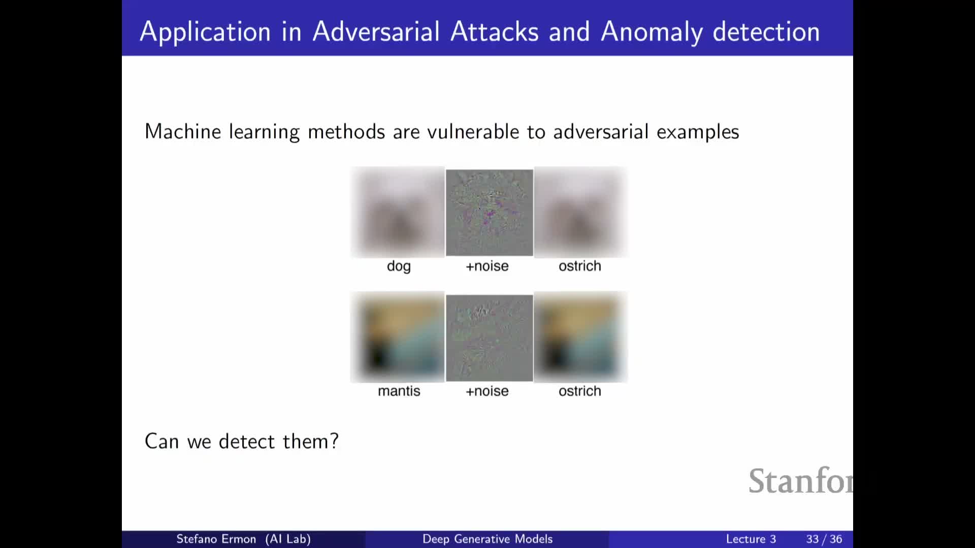
Autoregressive generative models assign a likelihood to each input via the product of conditionals, enabling applications such as anomaly detection by thresholding model likelihoods.
- Inputs with substantially lower likelihood than typical training data can be flagged as anomalous.
- Pixel-level models trained by maximum likelihood have demonstrated separation between natural images and adversarially perturbed images in likelihood histograms (often reported in bits per dimension), indicating learned conditionals capture subtle pixel dependencies.
- While likelihood-based defenses are not universally robust to adaptive attacks, pre-trained autoregressive models can still provide a practical mechanism for detecting certain classes of distributional shifts and adversarial perturbations.
Learning begins with defining objectives and the desiderata for model approximation; density estimation is a canonical target
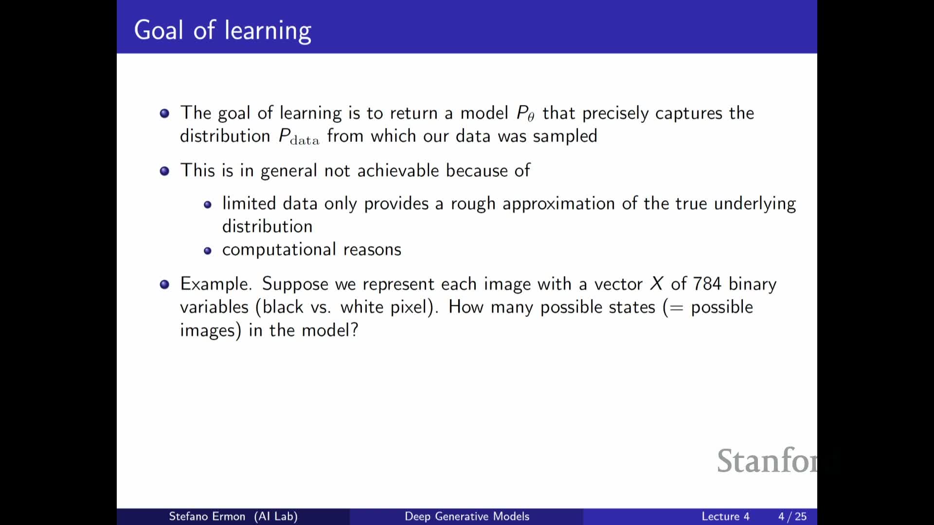
The learning problem specifies:
- A family of parameterized distributions,
- A dataset of i.i.d. samples drawn from an unknown data distribution, and
-
A notion of similarity or distance between distributions to guide parameter selection.
- A canonical goal is density estimation—approximating the full joint distribution so likelihoods and conditionals are accurate for downstream tasks such as sampling, conditioning, and anomaly detection.
- Alternative objectives may focus on task-specific conditionals or discriminative objectives when the full joint is not required.
The Kullback–Leibler divergence quantifies distributional discrepancy and has an information-theoretic compression interpretation
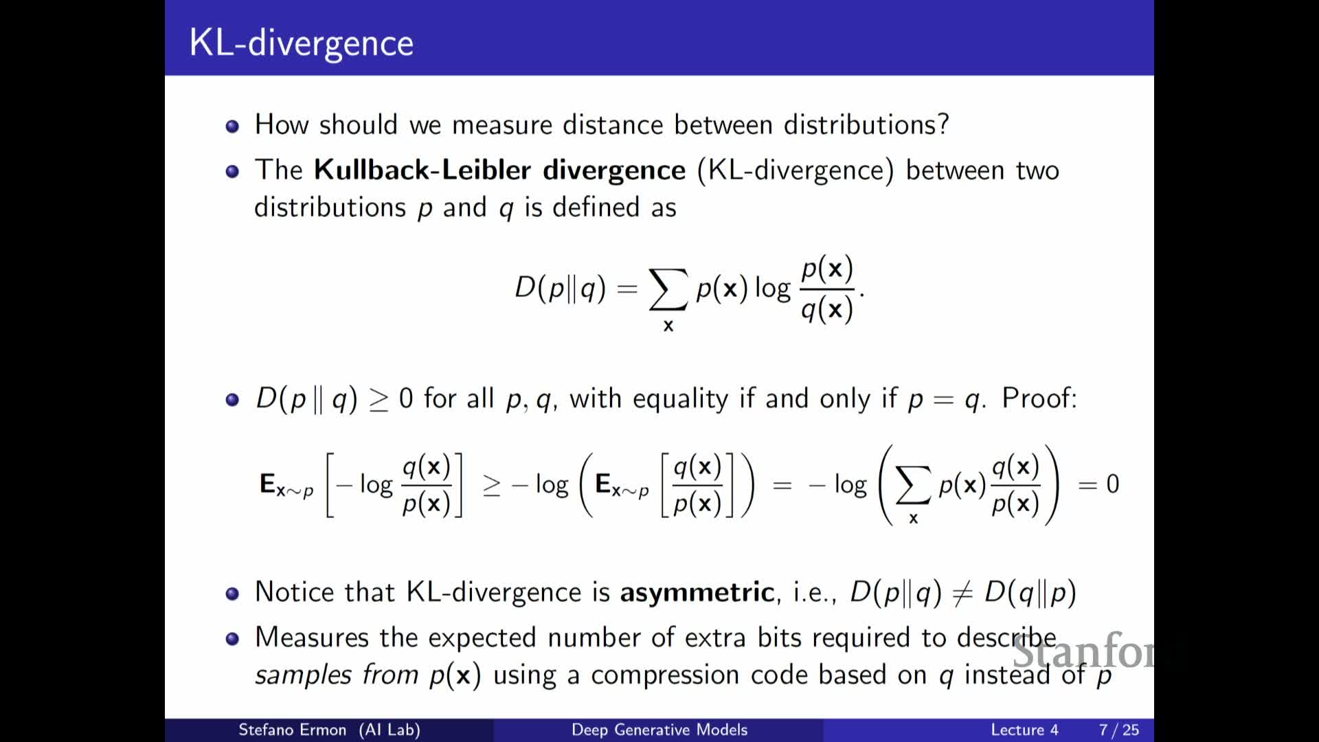
The KL divergence D_KL(p || q) = E_p[log p(x)/q(x)] measures how much the model distribution q diverges from the data distribution p by averaging log-probability ratios under p.
- KL is nonnegative and equals zero iff p = q almost everywhere.
-
It has an operational interpretation in terms of coding inefficiency: using codes optimized for q instead of the true p incurs an expected excess code length equal to D_KL(p q). - KL is asymmetric; choosing which argument is the data distribution versus the model (forward vs reverse KL) induces different behaviors:
-
**Forward KL (D_KL(p q))** tends to be mass-covering, encouraging q to cover p’s support. -
**Reverse KL (D_KL(q p))** tends to be mode-seeking, focusing q on high-density modes of p.
-
Minimizing forward KL between the data distribution and model reduces to maximizing expected log-likelihood under the data and yields maximum likelihood estimation
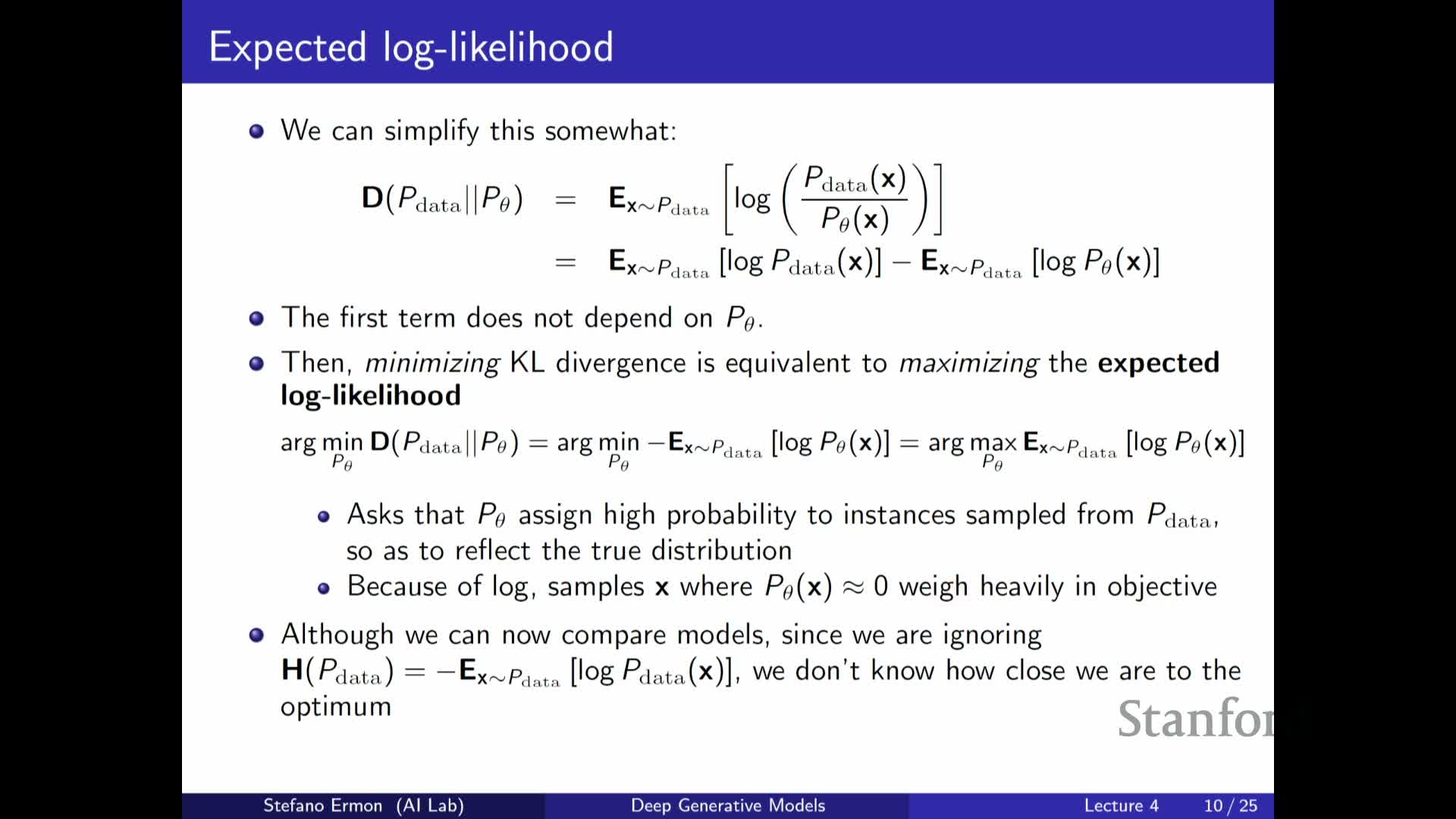
By expanding D_KL(p_data || p_theta) = E_p_data[log p_data(x) - log p_theta(x)] and noting the first term does not depend on theta, minimizing KL over theta is equivalent to maximizing E_p_data[log p_theta(x)] — the expected log-likelihood.
- In practice, the expectation under the unknown data distribution is approximated with the empirical average over the dataset, producing the maximum likelihood objective: maximize the average log probability that the model assigns to training samples.
- This connects an information-theoretic divergence minimization principle to the practical training objective used for autoregressive models.
The empirical average (Monte Carlo) approximates expectations and yields the practical MLE objective implemented as negative log-likelihood over the dataset
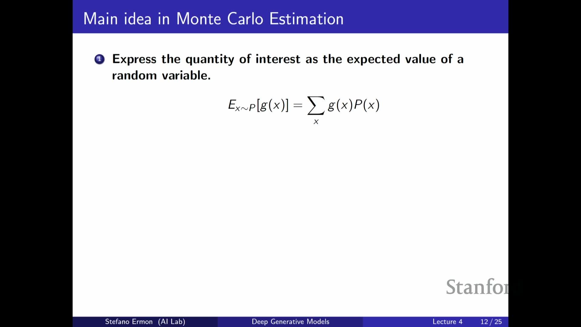
The expectation E_p_data[log p_theta(x)] is approximated by the sample average (1/N) sum_{i=1}^N log p_theta(x^{(i)}), a Monte Carlo estimator of the population objective.
- For autoregressive models each log p_theta(x^{(i)}) decomposes into a sum of conditional log-probabilities via the chain rule.
- Consequently, the dataset log-likelihood reduces to summing cross-entropy losses for the per-step conditionals across examples and positions.
- Maximizing this empirical log-likelihood is the standard MLE procedure, implemented in practice by minimizing the negative log-likelihood (cross-entropy) over the training set.
Gradient-based optimization of autoregressive models uses backpropagation and stochastic minibatch estimates for scalability
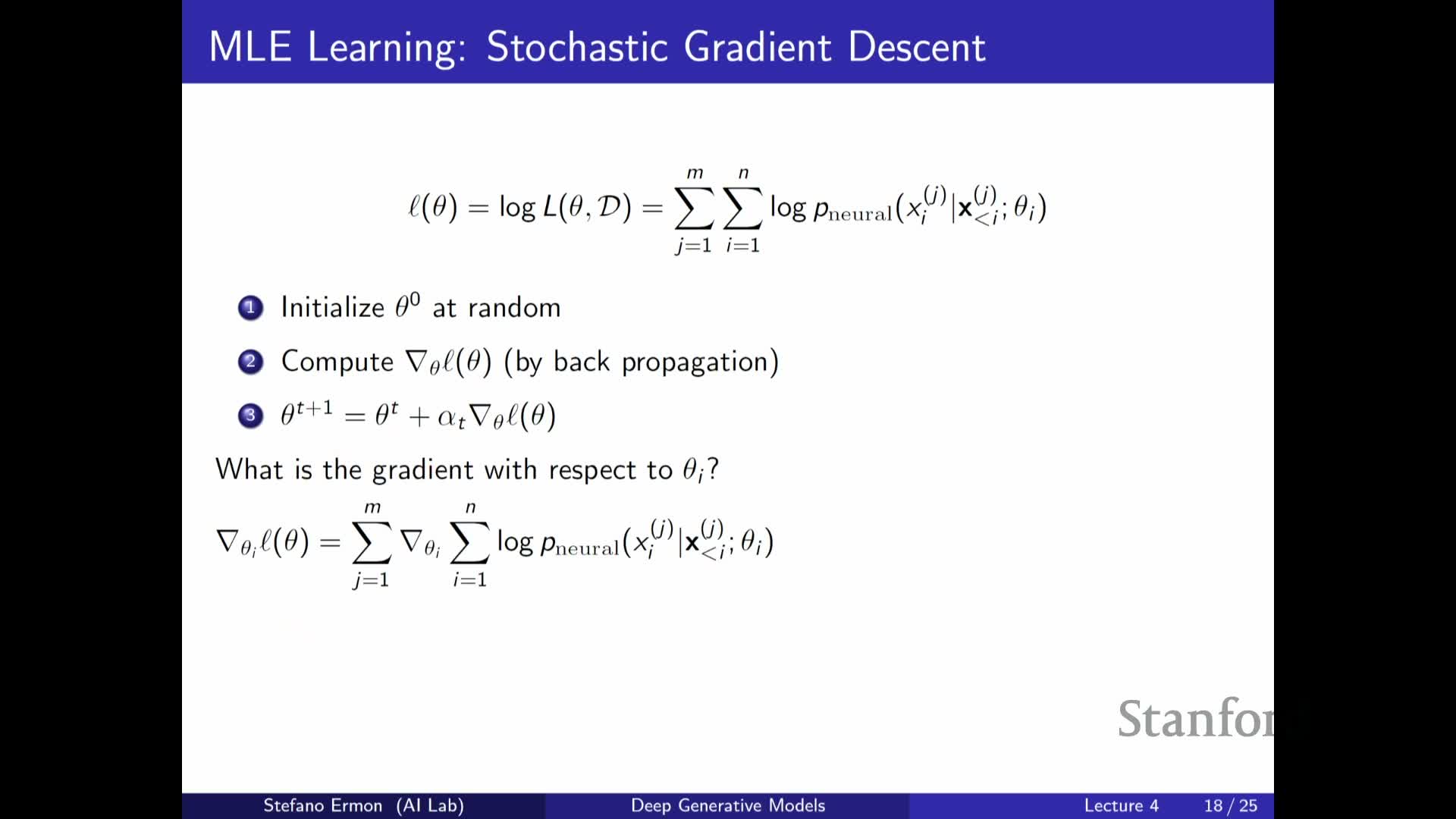
Closed-form solutions rarely exist for high-dimensional neural models, so parameters are optimized via gradient-based methods (e.g., stochastic gradient descent variants) using gradients computed by backpropagation through the network that parameterizes the conditionals.
- The full-dataset gradient is an expectation over the empirical distribution and is approximated with minibatch Monte Carlo: gradients are computed on small random subsets of training examples to produce unbiased, lower-cost gradient estimates for parameter updates.
- Parameter sharing across conditionals (e.g., through a single neural network) is standard.
- Training leverages parallel computation for per-minibatch forward/backward passes while preserving the autoregressive decomposition in the loss.
Generalization requires controlling model complexity via regularization, validation, and bias–variance trade-offs
Blindly maximizing empirical likelihood can lead to memorization and poor generalization on unseen samples; practitioners therefore apply regularization and model-selection practices to improve robustness.
- Common strategies:
- Constrain the hypothesis class or add regularization terms (e.g., weight decay),
- Use held-out validation sets for model selection,
- Apply early stopping and parameter sharing.
- The bias–variance trade-off guides choices: overly restrictive models exhibit bias (underfitting), while overly flexible models exhibit variance (overfitting).
- Practical mechanisms include cross-validation, monitoring validation loss, and using inductive biases that favor simpler or structured solutions to balance approximation capacity and robustness.
Enjoy Reading This Article?
Here are some more articles you might like to read next: