Stanford CS236- Deep Generative Models I 2023 I Lecture 5 - VAEs
- Autoregressive models factorize joint distributions using the chain rule and permit exact likelihood computation
- Latent variable models introduce unobserved variables Z to capture factors of variation in high-dimensional data
- Deep latent-variable models parametrize p(x|z) with neural networks that map Z to distribution parameters such as mu_theta and sigma_theta
- A mixture of Gaussians is a basic latent-variable model where Z is a categorical component index and p(x|z) is a Gaussian per component
- Prior choice, discrete vs continuous latents, and latent dimensionality determine inductive bias and expressiveness
- Marginal likelihood p(x) requires summing or integrating over Z and is generally intractable, motivating Monte Carlo estimators, importance sampling, and the Evidence Lower Bound (ELBO)
Autoregressive models factorize joint distributions using the chain rule and permit exact likelihood computation
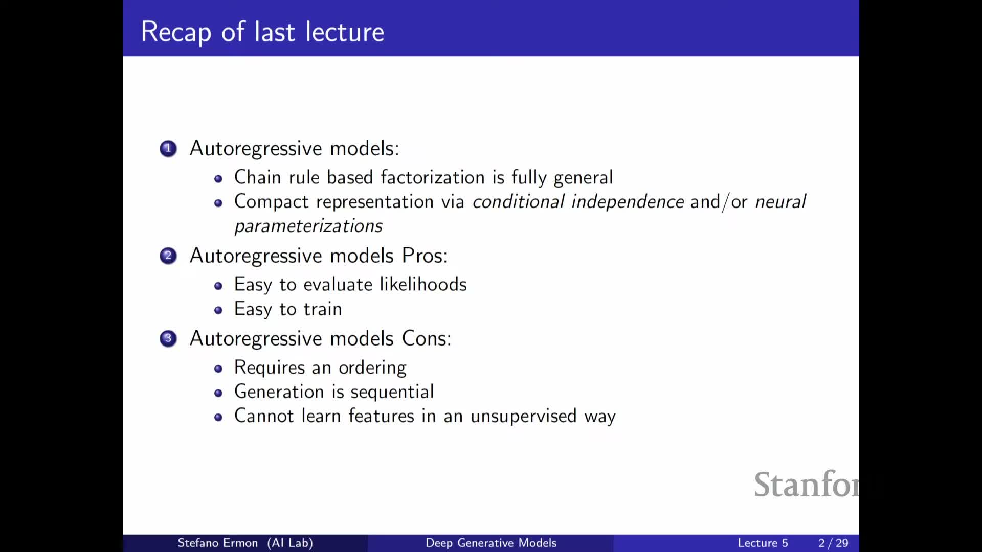
Autoregressive models represent the joint probability of a high-dimensional observation via the chain rule: p(x) = Π_t p(x_t | x_{<t}).
Neural architectures such as RNNs, CNNs, and Transformers are used to parameterize those conditionals and to capture both local and long-range dependencies.
Because the model defines an explicit factorization, the likelihood of any datum can be evaluated exactly and training by maximum likelihood is straightforward—this enables applications such as anomaly detection.
Key practical limitations include:
-
Ordering commitment: the model requires choosing an ordering of variables, which may be unnatural for some data.
-
Sequential ancestral sampling: generation is slow because samples are produced one variable at a time.
-
Feature extraction: it can be difficult to extract unsupervised feature representations directly from the model.
Latent variable models introduce unobserved variables Z to capture factors of variation in high-dimensional data
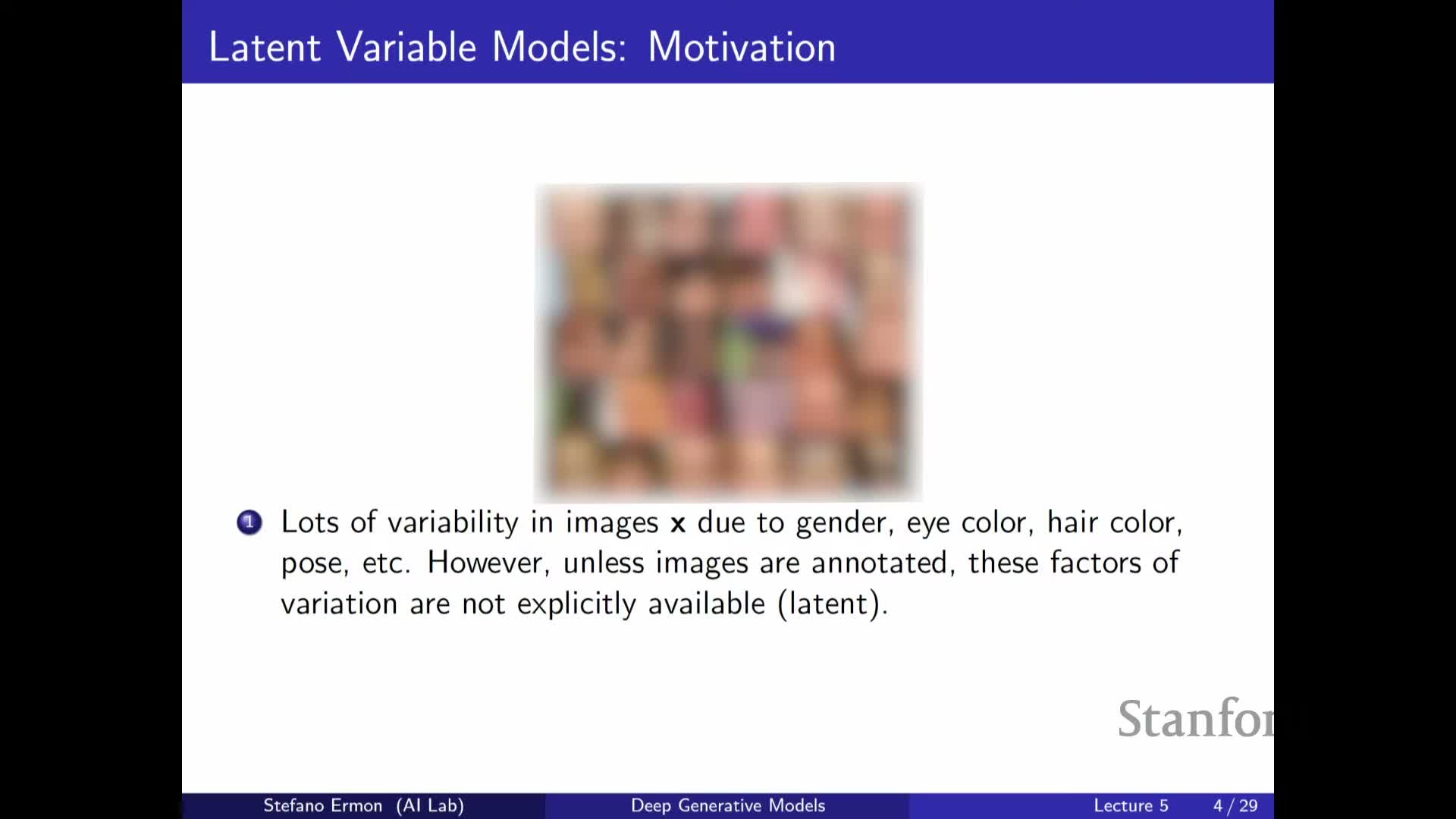
Latent variable models augment observed data X with latent random variables Z that represent underlying explanatory factors (for example, pose, age, or color for images).
| The generative model defines a joint p(X, Z), typically via a simple prior p(Z) and a conditional **p(X | Z)**, so the marginal over observations is **p(X) = ∫ p(X | Z) p(Z) dZ**. |
| Conditioning on Z can dramatically simplify modeling because **p(X | Z)** often captures narrower, less multimodal distributions—effectively implementing a clustering or mixture decomposition of the data. |
Learning and inference in these models enable representation learning by inferring Z for new X, which is useful for downstream tasks such as:
-
Classification
-
Transfer learning
-
Interpretable analysis of variation
Deep latent-variable models parametrize p(x|z) with neural networks that map Z to distribution parameters such as mu_theta and sigma_theta
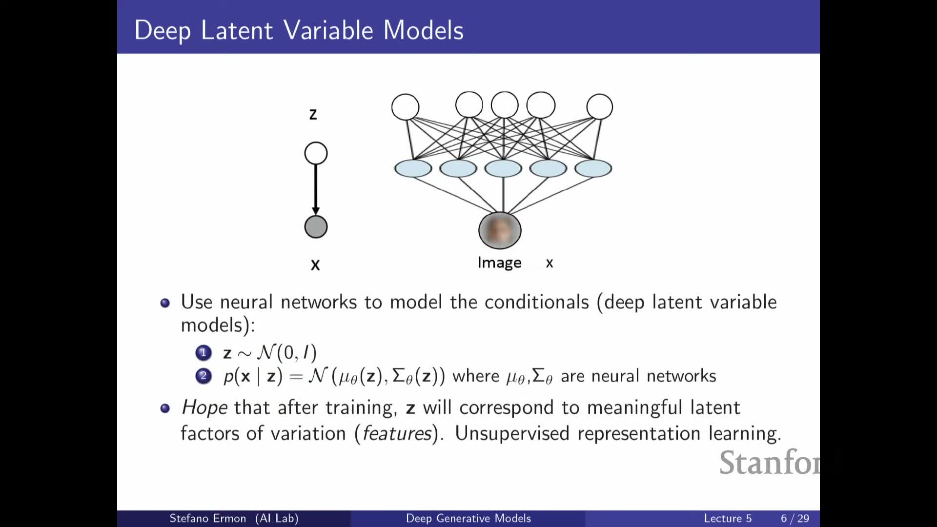
Deep latent-variable models typically choose a simple prior p(Z) (for example, a standard Gaussian) and model p(X | Z) by passing Z through neural network decoders that output parameters of a simple distribution (for example mean μ_θ(Z) and diagonal covariance σ_θ(Z) for a Gaussian likelihood).
Sampling proceeds in a clear sequence:
- Draw Z ∼ p(Z).
- Compute distribution parameters via the neural network decoders (e.g., μ_θ(Z), σ_θ(Z)).
-
Sample **X ∼ p(X Z)** using those parameters.
| Although **p(X | Z)** is simple, integrating over the continuous space of Z yields a highly expressive marginal p(X) that behaves like an infinite mixture model: the flexibility comes from the neural mapping from Z to component parameters rather than an explicit lookup for each component. |
The primary learning challenge is that Z is unobserved during training, so estimating model parameters requires methods to approximate or infer the latent values for each observed X.
A mixture of Gaussians is a basic latent-variable model where Z is a categorical component index and p(x|z) is a Gaussian per component
A Gaussian mixture model (GMM) is a shallow latent-variable model in which Z is a discrete categorical variable indexing K components and p(X | Z = k) = N(X; μ_k, Σ_k).
The generative process is:
- Sample component index k ∼ Categorical(π).
- Sample X ∼ N(μ_k, Σ_k).
The marginal is p(X) = Σ_k π_k N(X; μ_k, Σ_k), a weighted sum of Gaussians that enables multimodal densities and a clustering interpretation: inferring Z given X assigns data points to mixture components.
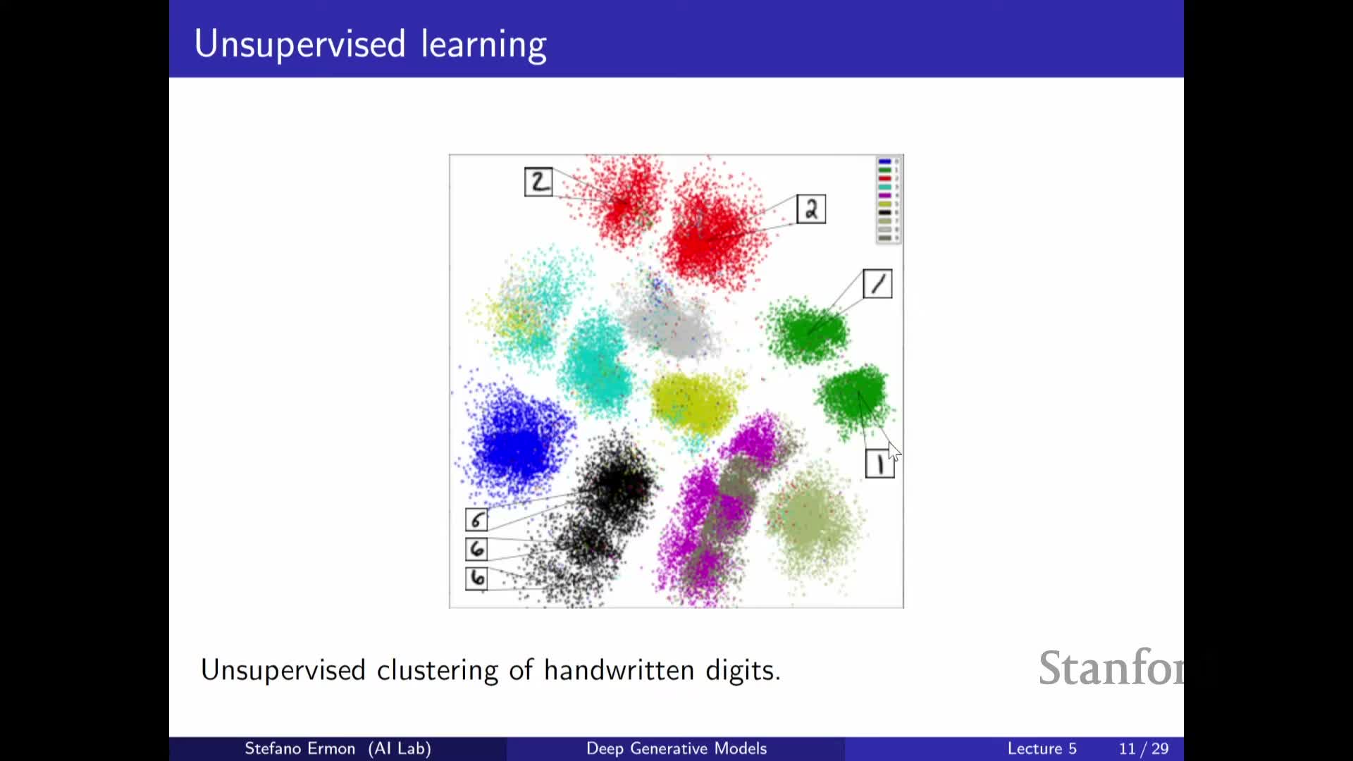
GMMs illustrate how simple conditionals can produce complex marginals and work well on low-dimensional data (examples include Old Faithful eruption data and low-dimensional projections of MNIST).
However, for high-dimensional data such as raw images, a GMM requires an impractically large K to model the manifold well and does not scale gracefully without adding structure or deep parameterizations.
Prior choice, discrete vs continuous latents, and latent dimensionality determine inductive bias and expressiveness
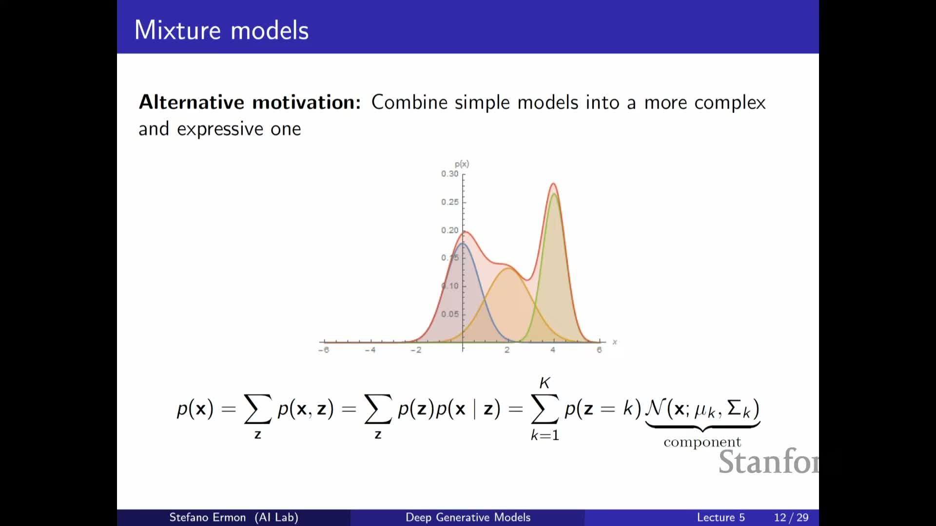
Design choices for p(Z) and the support of Z critically affect model behavior:
- Common priors: standard Gaussian, uniform, or learnable priors (including autoregressive priors over Z).
- Support of Z: discrete, continuous, or a combination.
-
Continuous Z gives an effectively infinite mixture because Z can take uncountably many values.
-
Discrete Z yields a finite mixture.
-
Continuous Z gives an effectively infinite mixture because Z can take uncountably many values.
- Dimensionality of Z (D_z) is a hyperparameter:
- Often D_z « D_x to compress factors of variation.
- In other paradigms, D_z can be equal to or greater than D_x.
- Often D_z « D_x to compress factors of variation.
These choices trade off interpretability, representational capacity, sampling convenience, and computational cost. Learning a richer prior or a mixture-of-priors can increase expressiveness when required.
Marginal likelihood p(x) requires summing or integrating over Z and is generally intractable, motivating Monte Carlo estimators, importance sampling, and the Evidence Lower Bound (ELBO)
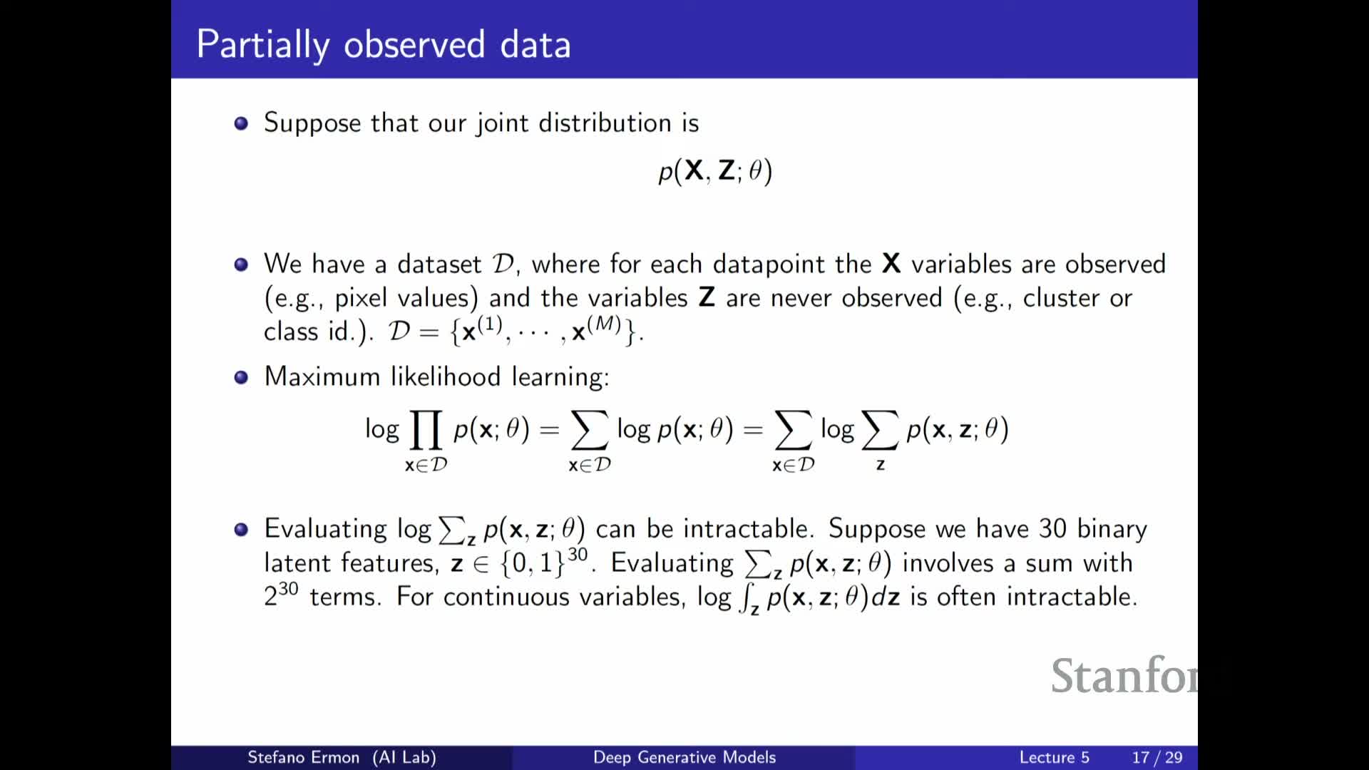
Computing the marginal p(X) = ∫ p(X, Z) dZ (or a sum over discrete Z) requires aggregating joint probabilities across all latent completions and becomes intractable for high-dimensional or continuous Z.
A naive Monte Carlo estimator that samples Z uniformly has prohibitive variance because most random completions have negligible joint probability; importance sampling reduces variance by drawing samples from a proposal distribution Q(Z) and reweighting by p(X, Z) / Q(Z).
Taking the logarithm of the marginal and exchanging log and expectation introduces bias, but Jensen’s inequality yields a tractable lower bound on the log marginal: the Evidence Lower Bound (ELBO).
The ELBO can be written as:
- An expectation under Q of log joint minus log Q (i.e., E_Q[log p(X, Z) − log Q(Z)])
- Equivalently, as the expected log joint under Q plus the entropy of Q.
| The ELBO is tight when **Q = p(Z | X). Maximizing the ELBO jointly over the generative parameters and the proposal/inference distribution **Q provides a practical objective for learning deep latent-variable models such as the variational autoencoder (VAE). |
Enjoy Reading This Article?
Here are some more articles you might like to read next: