Stanford CS236- Deep Generative Models I 2023 I Lecture 6 - VAEs
- Lecture agenda for completing the variational autoencoder exposition
- Variational autoencoder generative model samples a latent Z from a simple prior then decodes it to produce X
- VAE marginal distribution is highly flexible because it acts like an infinite mixture of conditionals indexed by Z
- Latent variables enable unsupervised discovery of structure and generalize clustering methods
- Training latent-variable models is challenging because marginal likelihood evaluation is expensive
- Prior over Z can be learned or structured hierarchically to increase model capacity
- Increasing decoder depth differs qualitatively from adding latent mixture components or stacking VAEs
- Variational inference introduces an auxiliary approximate posterior Q to obtain a tractable lower bound (ELBO)
- The ELBO decomposes into a reconstruction-like term plus an entropy (or divergence) term
- The ELBO becomes exact if Q equals the true posterior p(z|x), establishing a connection to EM
- The ELBO gap equals the KL divergence between the approximate and true posterior
- The practical approach is to optimize the ELBO over a parameterized family Q and the model p jointly
- Computing the posterior would allow exact maximum likelihood but is a chicken-and-egg problem
- Variational parameters parameterize a family of distributions used to approximate the posterior
- Latent dimensionality need not match data dimensionality and Q is often chosen Gaussian in VAEs
- The training objective is the dataset average ELBO and requires a per-datapoint posterior approximation
- Per-example variational parameters are conceptually optimal but not scalable, illustrated by a missing-pixel example
- Optimizing the ELBO can be done by coordinate or joint gradient-based updates but may not always increase true likelihood
- Monte Carlo sampling approximates intractable expectations in the ELBO using samples from Q
- Variational family choice must permit efficient sampling and probability evaluation
- Gradient with respect to decoder parameters is straightforward, but gradients with respect to variational parameters are challenging
- Score-function estimators (REINFORCE) and the reparameterization trick provide two approaches to gradients through stochastic nodes
- The reparameterization trick rewrites stochastic sampling as deterministic transformation of fixed noise to enable backpropagation
- Reparameterization does not apply to discrete latents; other estimators or relaxations are required
- Amortized inference uses an encoder neural network to predict variational parameters given X
- Training the encoder and decoder jointly with reparameterization yields scalable VAE learning
- ELBO can be interpreted as a regularized autoencoding objective, giving VAEs an autoencoder flavor
Lecture agenda for completing the variational autoencoder exposition
The lecture frames the plan to complete the exposition of the variational autoencoder (VAE) by focusing on the ELBO, practical optimization strategies, and links to classical autoencoders.
The goals are to explain why the model is called variational, how an autoencoder can be converted into a generative model, and to present both conceptual derivations and practical algorithmic solutions for training VAEs.
This framing sets expectations for subsequent sections on model structure, inference, and optimization.
Variational autoencoder generative model samples a latent Z from a simple prior then decodes it to produce X

VAE generative model (high-level recipe):
- Sample a latent variable Z from a simple prior, e.g. a multivariate standard Gaussian p(z).
-
Map Z through neural networks (the decoder) that output parameters of the conditional distribution **p(x z)** — typically a mean vector and a covariance or diagonal variance for a Gaussian likelihood.
-
Generate data X by sampling from that conditional **p(x z)**.
| The decoder networks are parameterized by model parameters θ, and the marginal p(x) is obtained by integrating **p(x | z) p(z)** over z. |
Despite the simple prior and conditionals, this construction yields a highly flexible marginal distribution over X because the neural decoder can produce complex, data-dependent likelihood parameters.
VAE marginal distribution is highly flexible because it acts like an infinite mixture of conditionals indexed by Z
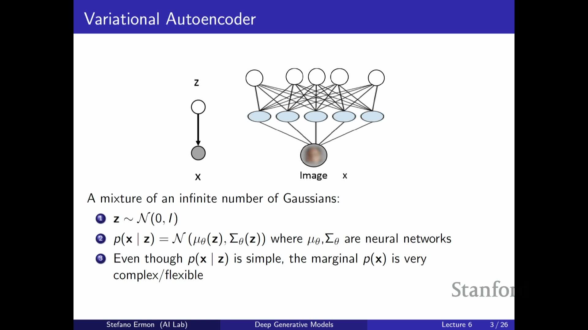
Because each latent value Z induces a different conditional p(x|z), the marginal p(x) is effectively a continuous (infinite) mixture of those conditionals weighted by the prior p(z).
- This mixture perspective explains how simple component distributions combine to yield a complex overall density over data.
- Integrating over all z enables expressive modeling of multimodal and otherwise complicated data distributions.
- It motivates treating Z as latent factors that capture salient variation across examples.
Latent variables enable unsupervised discovery of structure and generalize clustering methods

Latent-variable generative models like VAEs enable unsupervised learning by inferring Z from observed X, thereby discovering latent factors that explain data variability.
- Inferring Z can reveal semantic or statistical structure richer than simple clustering (e.g., k-means) because Z can be continuous, high-dimensional, and parameterized by neural networks.
- The inferred representations support downstream tasks such as:
- Interpolation in latent space,
- Generation of new samples,
-
Disentanglement of underlying factors.
This unsupervised representation learning is a principal motivation for VAEs.
Training latent-variable models is challenging because marginal likelihood evaluation is expensive
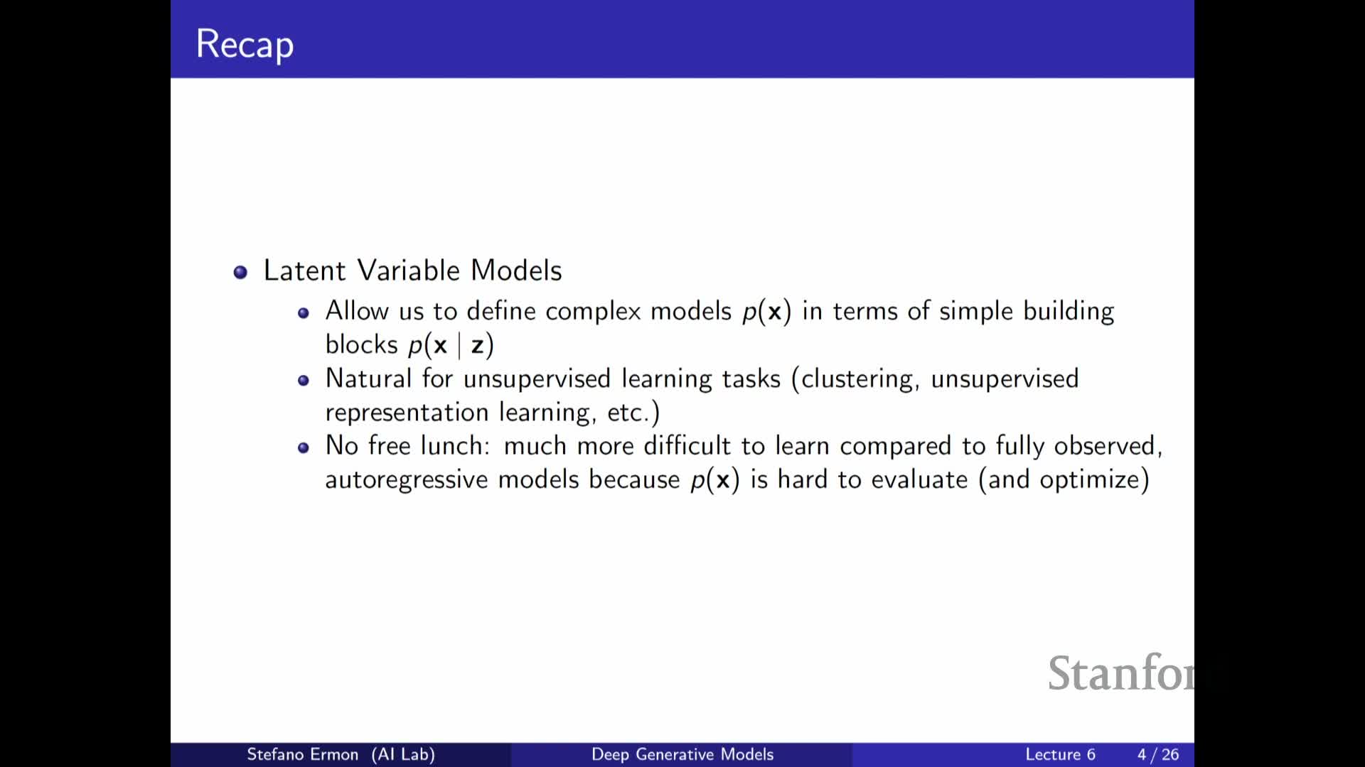
Maximum likelihood training requires evaluating the marginal p(x)=∫ p(x|z) p(z) dz, which is typically intractable because it integrates over all latent configurations Z.
- This intractability prevents direct computation of the likelihood and makes straightforward maximum likelihood optimization difficult or impossible for deep generative models.
- The difficulty contrasts with autoregressive models, where exact likelihood evaluation is tractable.
- This challenge motivates approximate inference methods such as variational inference, which provide tractable lower bounds on the marginal.
Prior over Z can be learned or structured hierarchically to increase model capacity
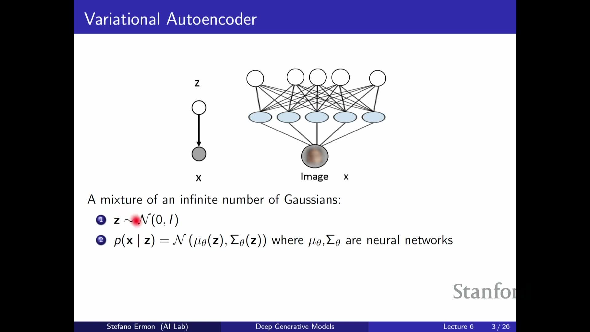
The prior p(z) need not be fixed — its parameters can be learned jointly with the decoder to increase expressiveness.
- Examples:
- Learn mean and covariance instead of fixing a standard Gaussian.
- Use hierarchical constructions: stack multiple latent-variable layers or VAEs so one latent variable is generated by another VAE.
- Learn mean and covariance instead of fixing a standard Gaussian.
- Stacking many layers can lead to models related to diffusion architectures.
Learning a richer prior or using hierarchical latents increases modeling power but typically increases inference and optimization complexity.
Increasing decoder depth differs qualitatively from adding latent mixture components or stacking VAEs
Depth in the decoder and richer latent structure are complementary design choices with different effects:
- Increasing decoder depth:
-
Makes **p(x z)** more expressive (the neural network can compute more complex conditional parameters). - Does not change the conditional family (e.g., it remains a Gaussian conditional if parameterized as such).
-
- Increasing latent dimensionality or stacking latent layers:
- Effectively adds more mixture components or hierarchical structure.
- Can qualitatively change the marginal p(x) and produce more multimodal behavior.
Thus, depth and latent complexity trade off different modeling effects and computational costs.
Variational inference introduces an auxiliary approximate posterior Q to obtain a tractable lower bound (ELBO)

Variational inference introduces an auxiliary distribution Q(z|x) to approximate the true posterior p(z|x) and uses Jensen’s inequality to derive an evidence lower bound (ELBO) on the marginal log-likelihood log p(x).
- The ELBO replaces the intractable marginal with a tractable objective that depends on expectations under Q and can be optimized.
- Training proceeds by jointly optimizing the generative parameters and the parameters of the approximate posterior to maximize the ELBO.
This reduces the missing-data learning problem to an optimization problem where both observed and imputed latent parts appear in a fully observed–like objective.
The ELBO decomposes into a reconstruction-like term plus an entropy (or divergence) term
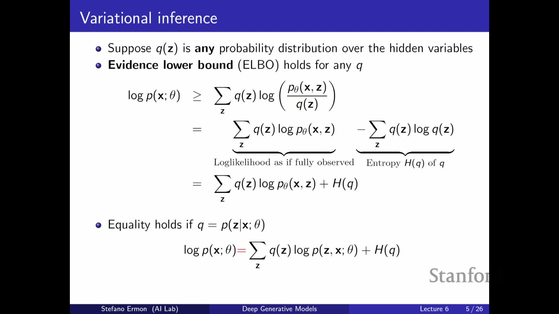
The ELBO can be written as the expected log joint under Q minus the expected log Q, equivalently as the expected log p(x,z) under Q plus the entropy of Q.
- First term: resembles a reconstruction or log joint likelihood when treating imputed Z as samples from Q; it encourages the decoder to assign high joint probability to those pairs (x, z).
- Second term: the entropy of Q (equivalently a negative KL contribution) encourages Q to be diffuse where appropriate.
Maximizing the sum of these two terms improves the lower bound and brings the approximate posterior closer to the true posterior.
The ELBO becomes exact if Q equals the true posterior p(z|x), establishing a connection to EM
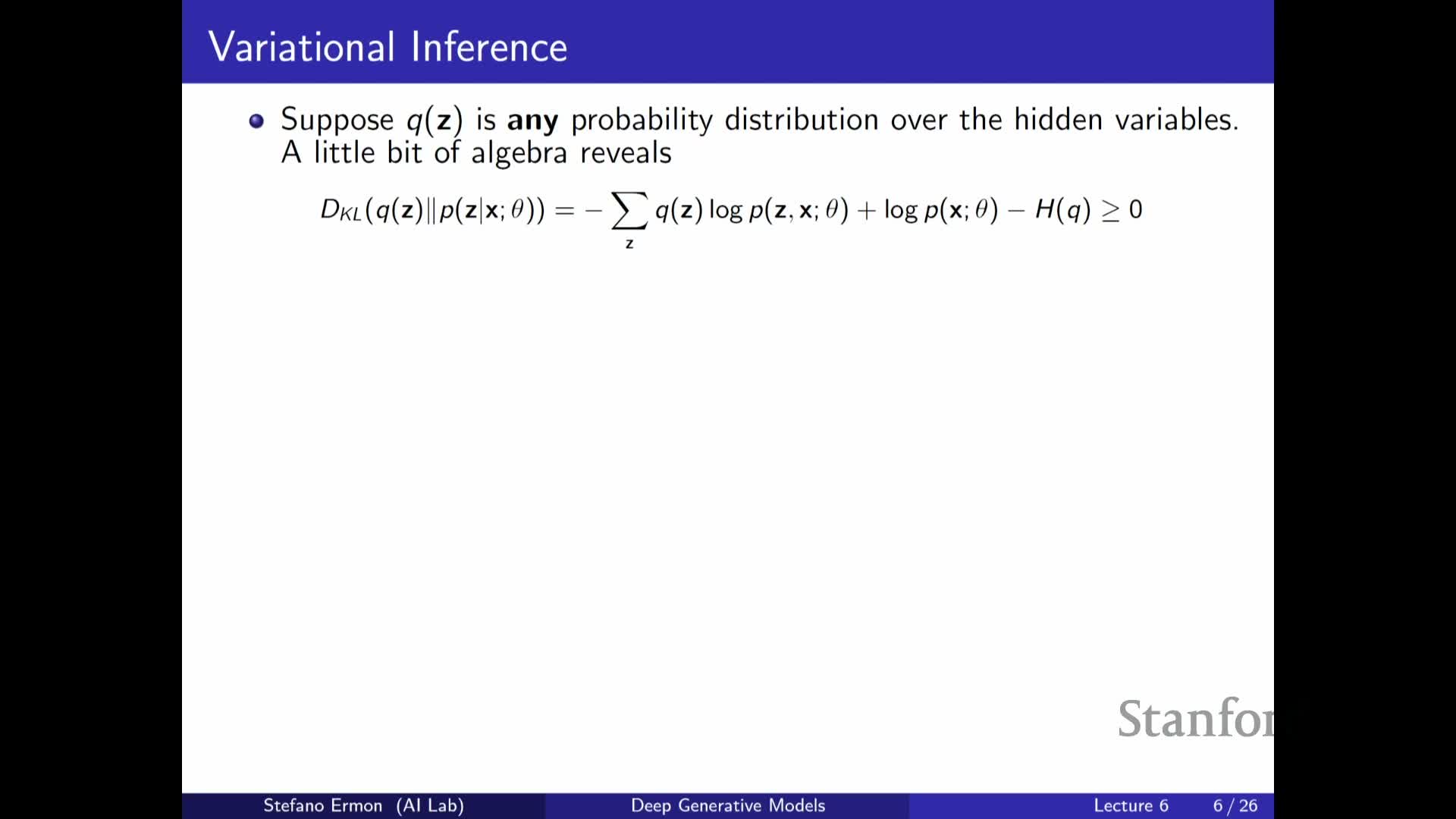
The ELBO inequality holds for any choice of Q, and it becomes tight exactly when Q(z|x) = p(z|x) under the current generative parameters.
- This shows the optimal auxiliary distribution is the exact posterior and connects variational learning to the Expectation-Maximization (EM) algorithm, whose E-step computes that posterior to obtain the tightest lower bound.
- In practice the true posterior is intractable and cannot serve directly as Q, but EM provides a conceptual reference point indicating the best achievable bound for a given generative model.
The ELBO gap equals the KL divergence between the approximate and true posterior
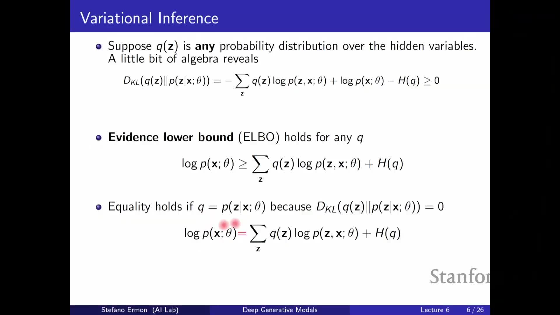
Rewriting the ELBO via KL divergence yields the identity:
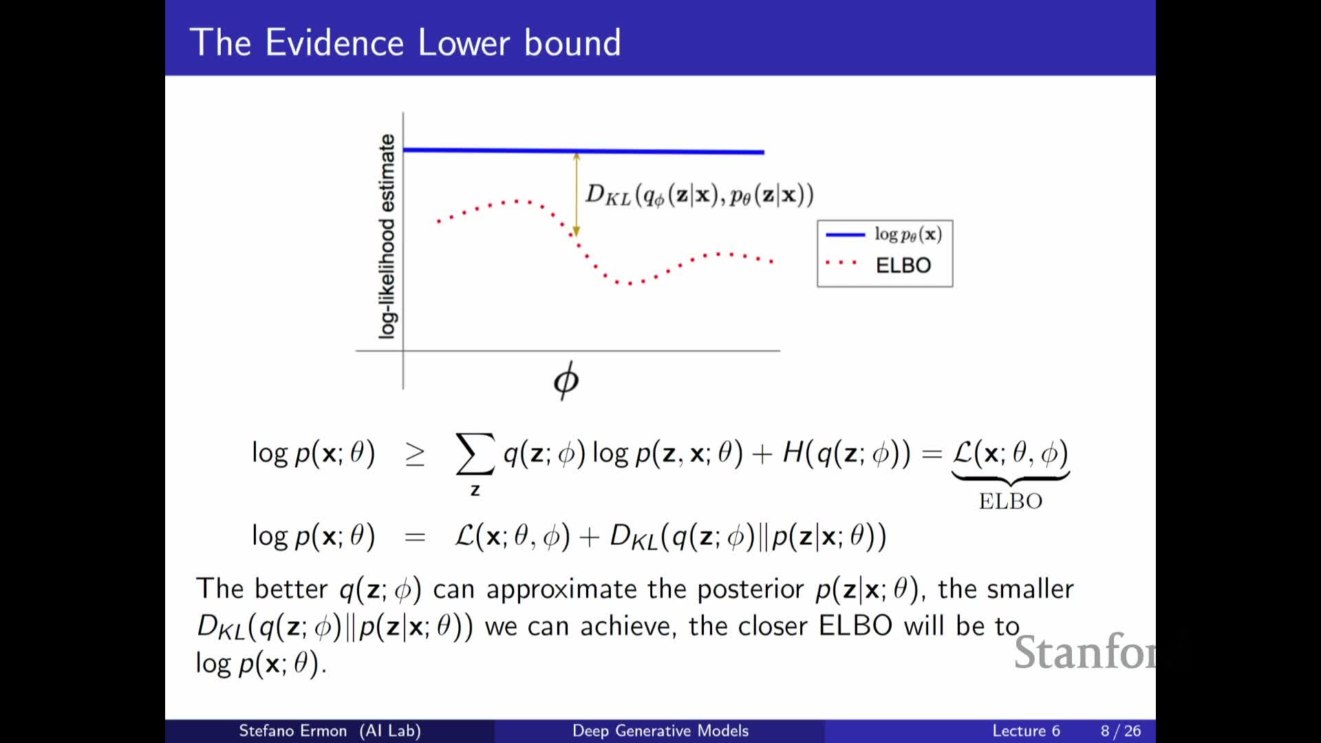
log p(x) = ELBO + KL(Q(z|x) || p(z|x)).
- The slack between log p(x) and the ELBO equals the nonnegative KL divergence, quantifying how loose the bound is.
-
Minimizing that KL tightens the ELBO toward the true marginal likelihood; when **Q = p(z x)** the KL is zero and the ELBO equals log p(x).
This identity motivates directly optimizing Q to reduce the KL gap as much as tractability allows.
The practical approach is to optimize the ELBO over a parameterized family Q and the model p jointly
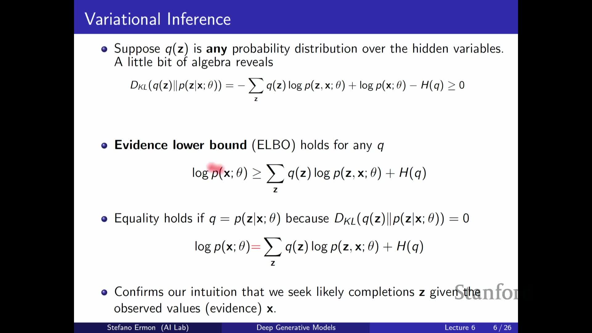
Because the exact posterior is intractable for most deep generative models, the practical procedure is variational inference: select a tractable parameterized family Q_φ(z|x) and jointly optimize model parameters θ and variational parameters φ to maximize the ELBO.
- Optimization searches for the tightest possible lower bound within the chosen family, effectively approximating the intractable expectation and enabling scalable learning.
- Joint optimization encourages the generative model to become compatible with an approximate posterior that can be evaluated and sampled efficiently, yielding a tractable surrogate objective for maximum likelihood.
Computing the posterior would allow exact maximum likelihood but is a chicken-and-egg problem
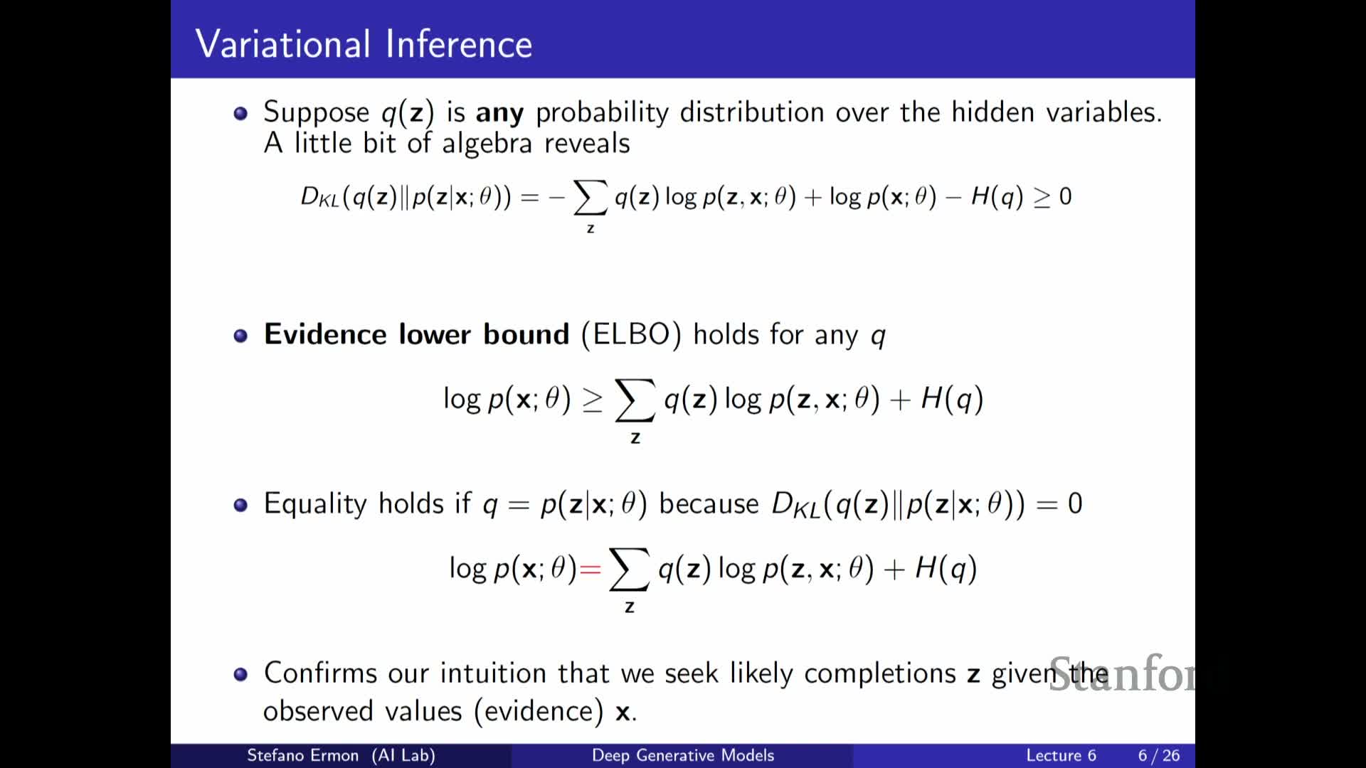
If one could compute the exact posterior p(z|x), maximizing the ELBO with that Q would be equivalent to maximizing log p(x), giving exact maximum likelihood estimation.
-
However, **p(z x)** depends on p(x) (the marginal likelihood), which is itself the optimization target, creating a circular dependence that prevents direct computation.
- Variational inference adopts a pragmatic strategy: optimize a tractable surrogate (the ELBO) while improving Q to approach the true posterior, trading exactness for computational tractability and providing guarantees in terms of KL divergence.
Variational parameters parameterize a family of distributions used to approximate the posterior
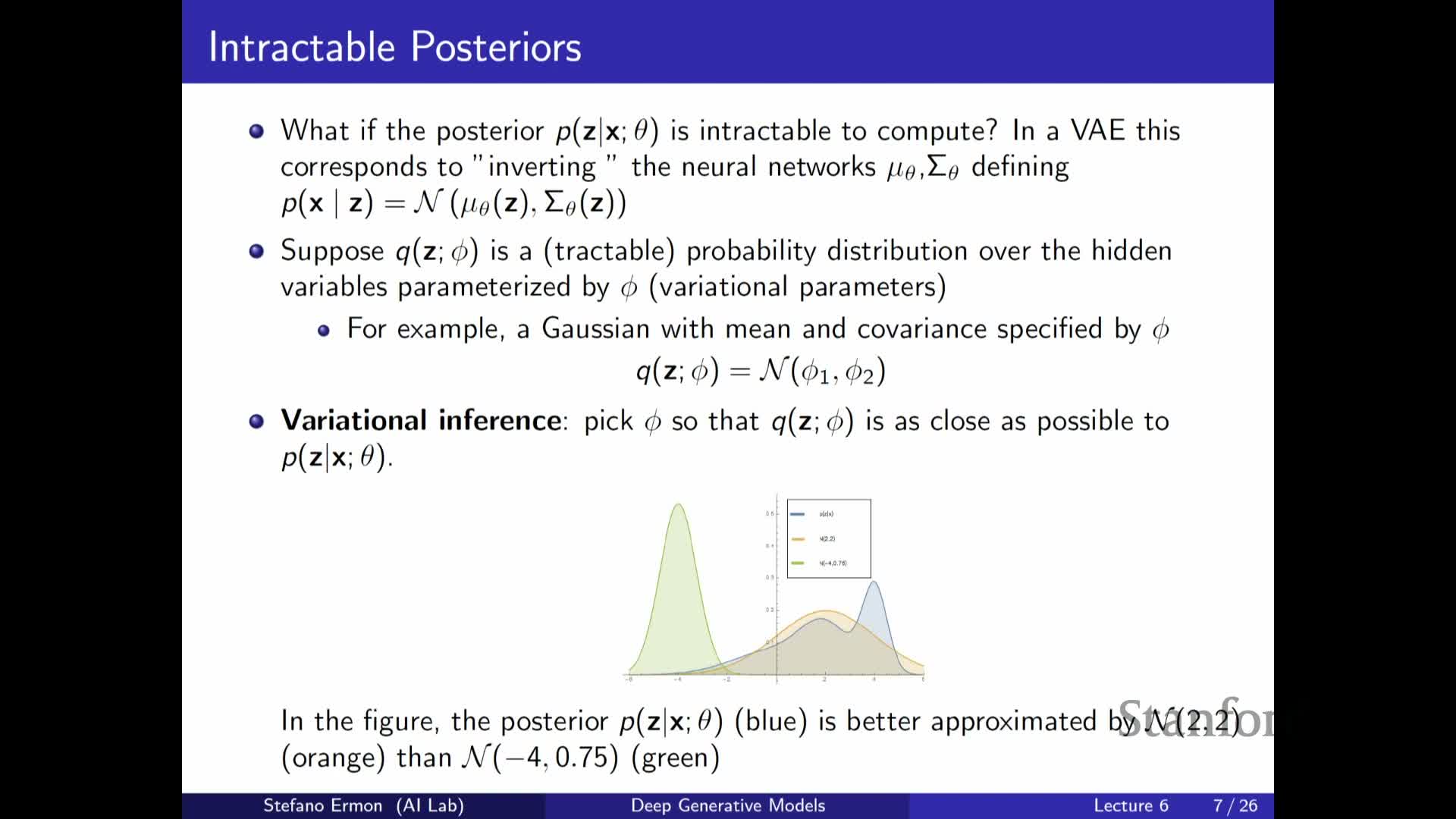
Variational inference specifies a family of approximating distributions Q_φ parameterized by φ (e.g., mean and covariance for Gaussians) and seeks φ that makes Q_φ close to the intractable posterior.
-
Example: choosing Q_φ to be Gaussian means φ contains the mean vector and covariance (or diagonal variance), and optimization tunes those parameters to approximate **p(z x)**.
- The family choice trades approximation capacity for tractability of sampling and density evaluation; an insufficiently expressive family can leave a large ELBO gap.
Latent dimensionality need not match data dimensionality and Q is often chosen Gaussian in VAEs

The latent-space dimensionality is an independent modeling choice and usually differs from the data dimension; the key requirement is that latent variables capture meaningful factors of variation.
-
In standard VAEs, **Q_φ(z x)** is commonly a multivariate Gaussian with diagonal covariance for tractability, and φ parameterizes its mean and log-variance.
- This Gaussian choice allows efficient sampling and analytic density evaluation, enabling scalable gradient-based optimization via the reparameterization trick.
Latent dimension and variational-family choices affect representation capacity and inference quality.
The training objective is the dataset average ELBO and requires a per-datapoint posterior approximation
Maximum likelihood for a dataset is the average log-likelihood across data points, and the ELBO provides a per-example lower bound that can be summed over the dataset.
-
The exact posterior **p(z x)** varies across data points, so the ideal variational approximation would use different φ_i for each data point to get the tightest per-example bound.
- Maintaining individual variational parameters for large datasets is not scalable, which motivates amortized inference where a shared function predicts per-example variational parameters.
Training therefore balances per-example tightness with global tractability.
Per-example variational parameters are conceptually optimal but not scalable, illustrated by a missing-pixel example
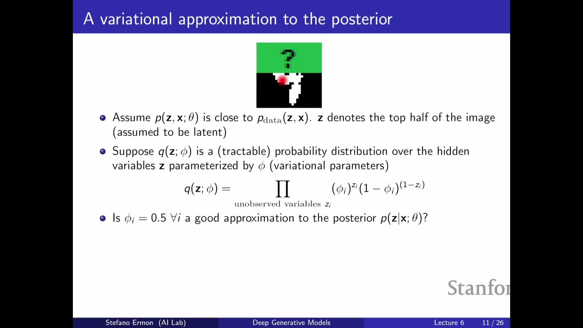
A conceptual (but impractical) approach is to allocate separate variational parameters for each data point and locally optimize them to obtain the tightest ELBO per example.
- This maximizes the sum-of-bounds objective but scales poorly with dataset size.
- The missing-pixels example illustrates that optimal guesses for missing values depend on the observed part of each image, so variational parameters must vary with x to capture that dependence.
Per-example optimization yields superior bounds but is impractical for large datasets and for online or test-time conditional likelihood evaluation, motivating amortized inference via a shared encoder.
Optimizing the ELBO can be done by coordinate or joint gradient-based updates but may not always increase true likelihood
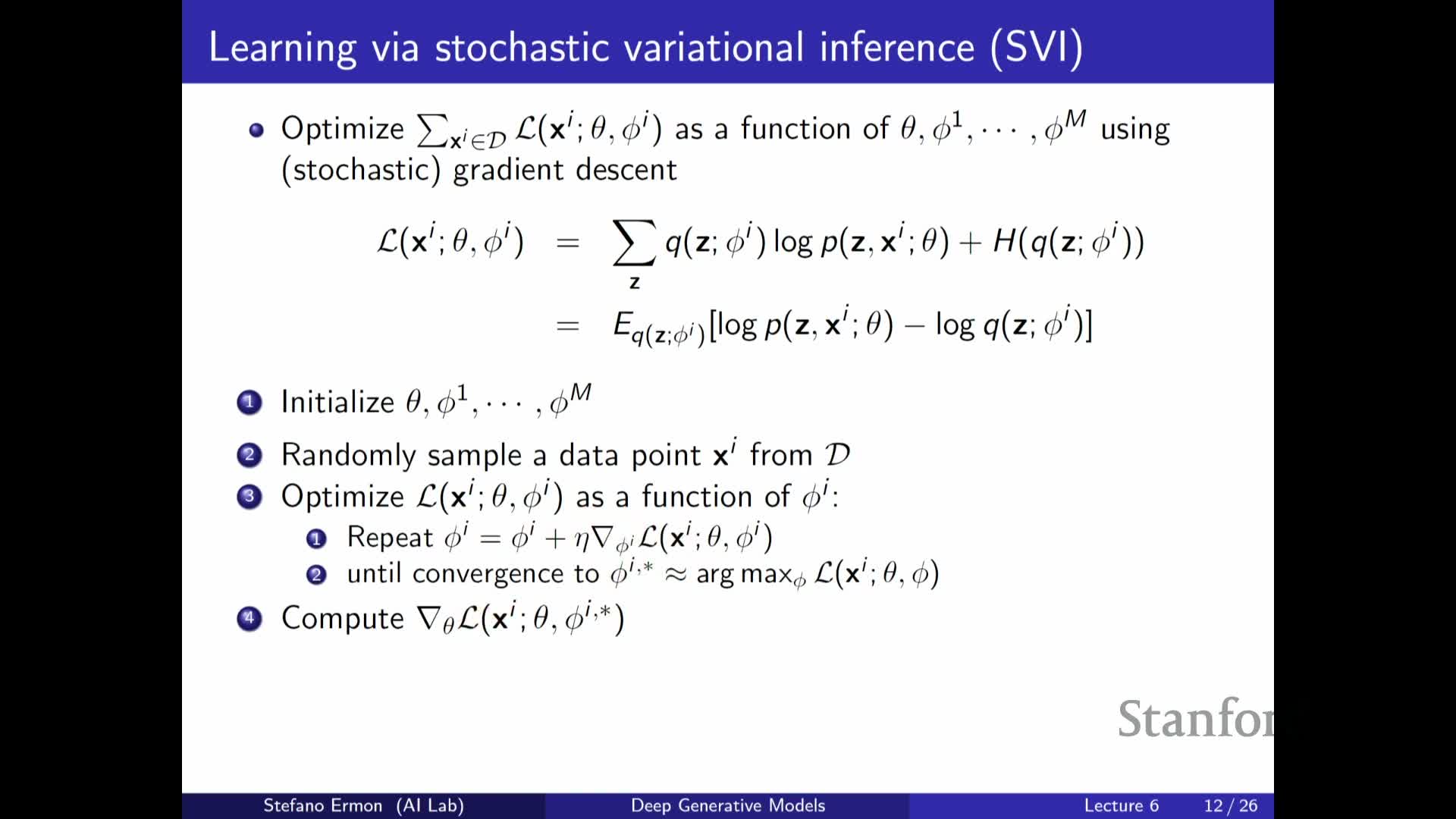
Practical optimization strategies include alternation and joint updates:
- Perform coordinate-ascent-like updates that alternately optimize variational parameters (or the encoder) and generative parameters.
- Or perform joint gradient-based updates on both θ and φ.
Caveats and trade-offs:
- Increasing the ELBO does not strictly guarantee that the true marginal likelihood increases monotonically because the bound can be loose; in some regions the ELBO can rise while the true likelihood falls.
- Choices such as performing multiple inner steps on variational parameters per outer model update influence convergence behavior and computational cost.
Monte Carlo sampling approximates intractable expectations in the ELBO using samples from Q
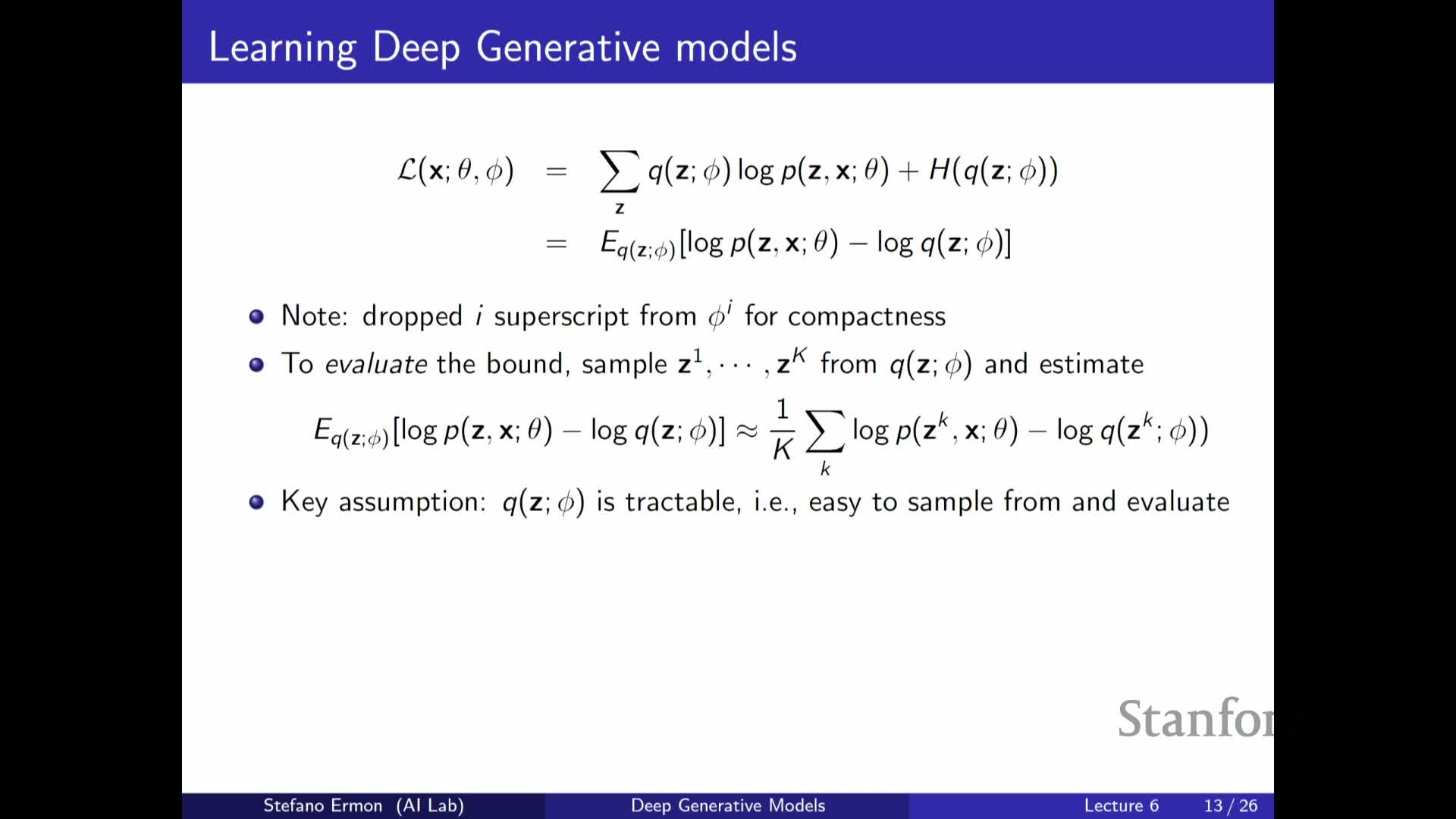
The ELBO contains expectations under Q_φ that are typically intractable to compute analytically, so Monte Carlo approximations are used:
-
Sample K latent draws from **Q_φ(z x)** and form empirical averages to approximate the expectations.
- In practice many implementations use K = 1 per example per update for computational efficiency, although larger K reduces estimator variance.
Efficient Monte Carlo requires that Q_φ supports both efficient sampling and tractable density evaluation; these constraints guide the choice of variational families. Sample-based estimators enable stochastic gradient optimization of the ELBO via autodiff frameworks.
Variational family choice must permit efficient sampling and probability evaluation
A practical variational family must allow two operations efficiently:
-
Sampling z ~ **Q_φ(z x)**, and
-
Computing **log Q_φ(z x)** for those samples.
Candidate families and considerations:
-
Factorized Gaussians — simple, efficient sampling and density evaluation.
-
Flow-based models — attractive because invertible transforms provide exact likelihoods and efficient sampling.
-
Autoregressive models — usable if both sampling and density evaluation are efficient.
-
GAN-style implicit models — typically do not provide tractable densities and are poor choices for Q.
The feasibility of gradient estimators and variance reduction techniques depends strongly on the chosen family.
Gradient with respect to decoder parameters is straightforward, but gradients with respect to variational parameters are challenging
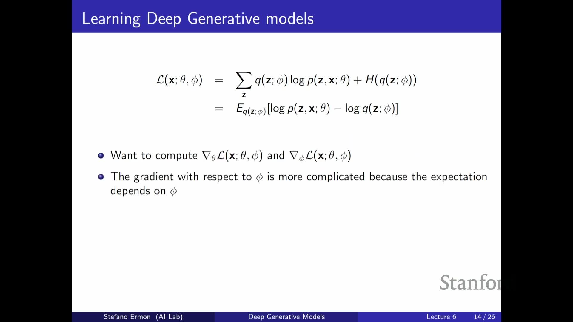
Gradients behave differently for decoder and encoder parameters:
- Gradient w.r.t. decoder parameters θ is straightforward because Q_φ does not depend on θ; sampled z can be treated as observed and one differentiates the log joint at those samples.
- Gradient w.r.t. variational parameters φ is challenging because the sampling distribution Q_φ depends on φ, so small changes in φ change the distribution of samples themselves.
This dependence complicates unbiased, low-variance gradient estimation and motivates specialized estimators such as score-function methods and the reparameterization trick.
Score-function estimators (REINFORCE) and the reparameterization trick provide two approaches to gradients through stochastic nodes

Two broad estimator families for gradients w.r.t. φ:
-
Score-function estimator (REINFORCE):
- Writes the gradient as an expectation of reward times the score function of Q.
- Generic but often high variance; requires variance-reduction techniques for practical use.
-
Reparameterization trick:
- Rewrites a sample z ~ Q_φ as a differentiable transformation z = g_φ(ε) of a parameter-free noise variable ε.
- Pushes dependence on φ inside a deterministic function and permits low-variance pathwise derivatives via backpropagation.
- Typically yields more efficient gradient estimates than REINFORCE when applicable (e.g., Gaussian families).
The reparameterization trick rewrites stochastic sampling as deterministic transformation of fixed noise to enable backpropagation
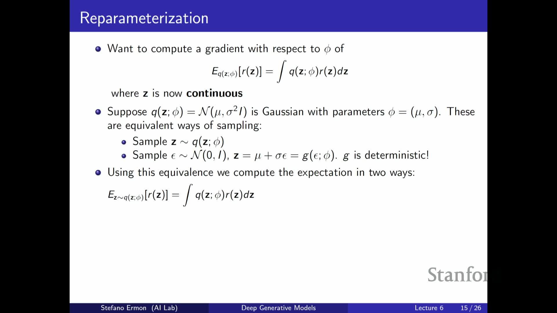
When samples can be expressed as z = g_φ(ε) with ε drawn from a fixed base distribution (e.g., standard normal), the expectation under Q_φ can be estimated by sampling ε and evaluating the deterministic transform:
- This representation removes the explicit dependence of the sampling measure on φ, allowing gradients to be moved inside the expectation and computed by autodiff through g_φ.
- The trick reduces gradient estimator variance and enables efficient end-to-end optimization of encoder parameters when latents are continuous and g_φ is differentiable.
Applicability requires that a differentiable reparameterization exists for the chosen variational family.
Reparameterization does not apply to discrete latents; other estimators or relaxations are required

The reparameterization trick relies on continuous differentiable transformations and therefore does not directly handle discrete latent variables (categorical, integer-valued Z).
Options for discrete latents include:
- Fall back to score-function estimators like REINFORCE.
- Use continuous relaxations (e.g., Gumbel-softmax).
- Design structured variational approximations and specialized estimators tailored to the discrete case.
Each choice trades off bias, variance, and computational tractability. Some continuous structured models (e.g., flows) extend the range of reparameterizable families and are used when possible.
Amortized inference uses an encoder neural network to predict variational parameters given X
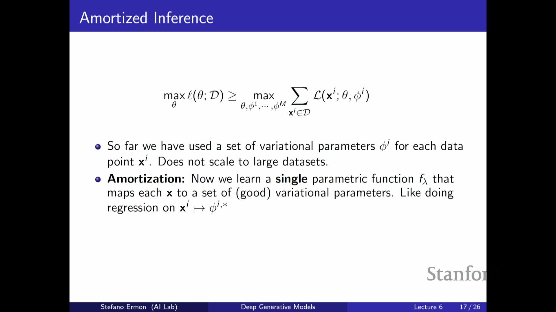
Amortized inference trains a parametric encoder q_φ(z|x) (a neural network) that maps each observed x to variational parameters (e.g., mean and variance of a Gaussian).
- The encoder amortizes the cost of per-example optimization by predicting an approximate posterior in a single forward pass, making training and test-time inference scalable.
- Benefits: reduced memory and computation, generalization to new datapoints without per-point optimization.
- Trade-off: constrains the family of approximate posteriors to those the encoder can represent.
In VAEs, the encoder is paired with a decoder and both are trained jointly to maximize the ELBO.
Training the encoder and decoder jointly with reparameterization yields scalable VAE learning
In practice, VAEs are trained by jointly optimizing decoder parameters θ and encoder parameters φ via stochastic gradient ascent on the ELBO, using the reparameterization trick to backpropagate through stochastic latents.
Typical minibatch training loop (per update):
- Sample a minibatch of data points x.
- Use the encoder to predict variational parameters (mean, log-var) for each x.
- Sample latent noise ε and transform to z = g_φ(ε) (reparameterization).
- Compute per-example ELBO terms (reconstruction + KL/entropy).
- Backpropagate gradients through both encoder and decoder and update φ and θ.
This joint optimization keeps encoder and decoder synchronized so the encoder tracks the changing posterior induced by the decoder and the decoder adapts to be compatible with the encoder — the standard scalable approach to fit deep VAEs.
ELBO can be interpreted as a regularized autoencoding objective, giving VAEs an autoencoder flavor
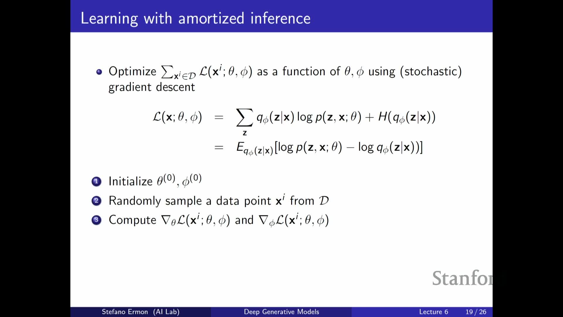
The ELBO has an interpretation analogous to an autoencoder loss plus regularization:
- The expected log likelihood term corresponds to a reconstruction objective of x from z.
- The KL (or entropy) term regularizes the approximate posterior to be close to the prior.
Consequences and intuition:
- This duality explains the description of VAEs as probabilistic (variational) autoencoders: an encoder produces latent codes and a decoder reconstructs data from codes.
- The probabilistic formulation makes uncertainty explicit, enables principled generation, and the regularization prevents pathological solutions.
In short, VAEs combine reconstruction-driven representation learning with a principled probabilistic latent-variable model.
Enjoy Reading This Article?
Here are some more articles you might like to read next: