Stanford CS236- Deep Generative Models I 2023 I Lecture 7 - Normalizing Flows
- Lecture plan and high-level VAE setup
- Monte Carlo estimation of the ELBO and stochastic encoding
- KL regularization to match the encoder to a prior and enable generation
- Optimization choices and discrete latents: REINFORCE and encoder flexibility
- Sampling at generation time and the role of the prior distribution
- Autoencoding interpretation, compression, and mutual information trade-offs
- Practical considerations: computing the ELBO, sampling strategies, and synthetic augmentation
- VAE training dynamics: posterior collapse, reconstruction weight, and sample diversity
- Flow models motivation: invertible latent-variable models with tractable likelihoods
- Change-of-variables in one dimension: CDF/PDF relationships and example transforms
- Linear multivariate transforms and the determinant of the Jacobian
- Nonlinear invertible mappings and the multivariate change-of-variables formula
Lecture plan and high-level VAE setup
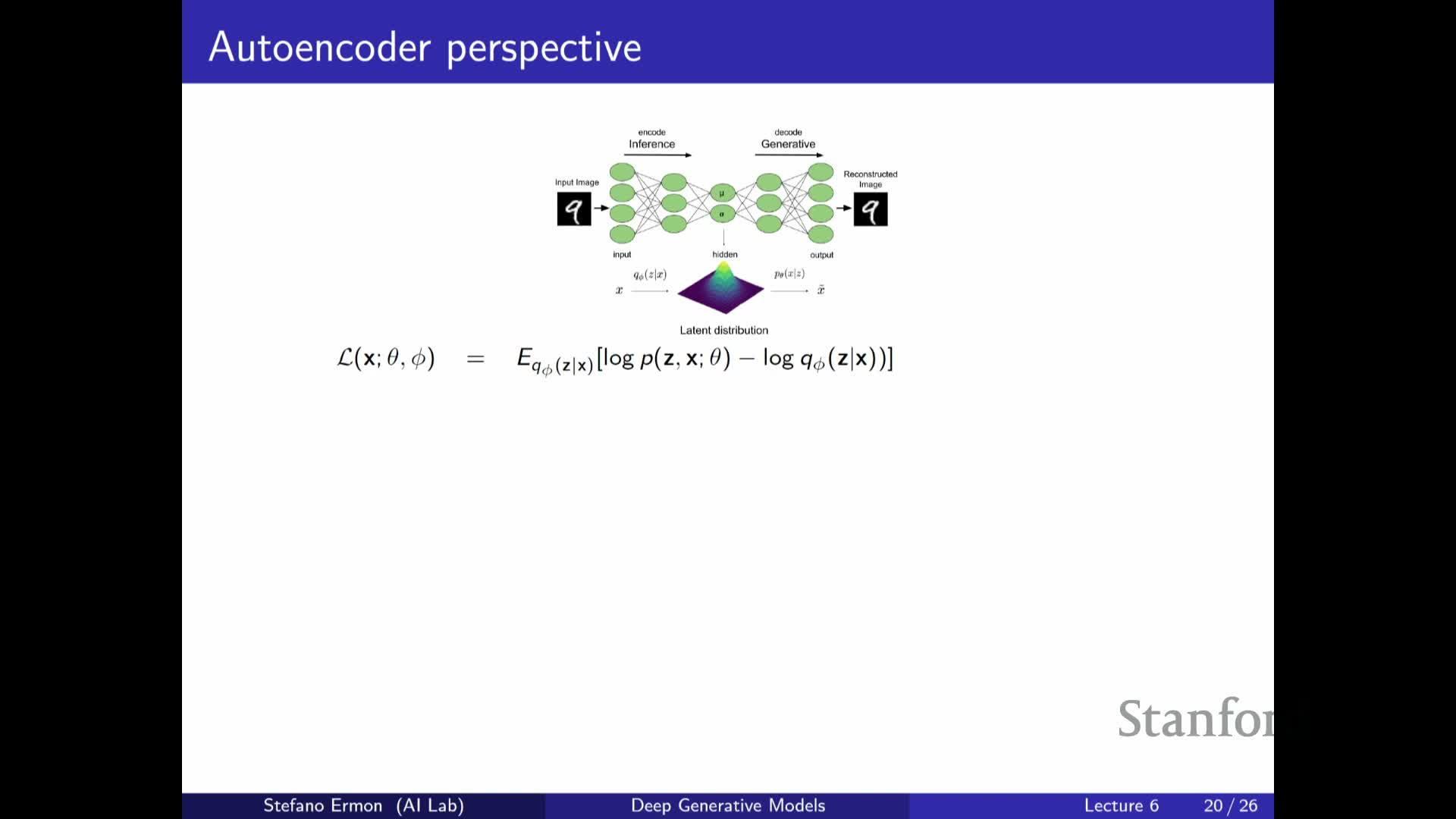
The lecture begins by outlining the plan to finish variational autoencoder (VAE) material and introduce flow models.
- A VAE is defined by:
-
A generative model **p_θ(x z)** (the decoder) that maps latents z to observations x.
-
An inference network **q_φ(z x)** (the encoder) that outputs variational parameters to approximate the true posterior **p(z x)**.
-
- Training optimizes the joint objective, the evidence lower bound (ELBO):
- The ELBO lower-bounds the marginal log-likelihood log p_θ(x).
- It is maximized with respect to both decoder (θ) and encoder (φ) parameters.
- Conceptual framing:
- View the encoder as a mapping that proposes plausible latent completions z for each observed x.
- The ELBO decomposes into an expected reconstruction term and a regularizing KL term that balances fidelity and prior conformity.
Monte Carlo estimation of the ELBO and stochastic encoding
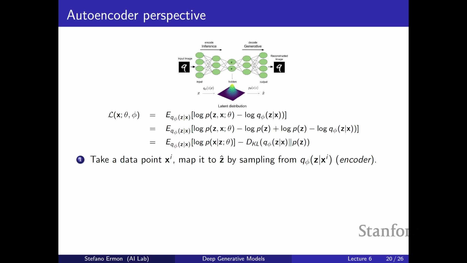
The ELBO expectation over q_φ(z|x) is typically approximated by Monte Carlo sampling from the encoder.
- When q is Gaussian:
- The encoder network emits mean and variance parameters.
- Samples of z are drawn accordingly (using reparameterization when available).
- Workflow for a sampled z:
-
Sample z ~ q_φ(z x). -
Pass the sampled z through the decoder **p_θ(x z)**. - The log-likelihood for the sampled z acts as a reconstruction objective for x.
- For Gaussian decoders, this corresponds to an L2-style reconstruction loss.
- For Gaussian decoders, this corresponds to an L2-style reconstruction loss.
-
- Implications:
- The encoder maps inputs to distributions over latents, not single deterministic codes.
- This allows the model to represent posterior uncertainty and multiple plausible explanations for x.
- Practical trade-offs:
- Monte Carlo estimates give unbiased loss and gradient estimates but require trading off sample count against computational cost.
- Monte Carlo estimates give unbiased loss and gradient estimates but require trading off sample count against computational cost.
KL regularization to match the encoder to a prior and enable generation
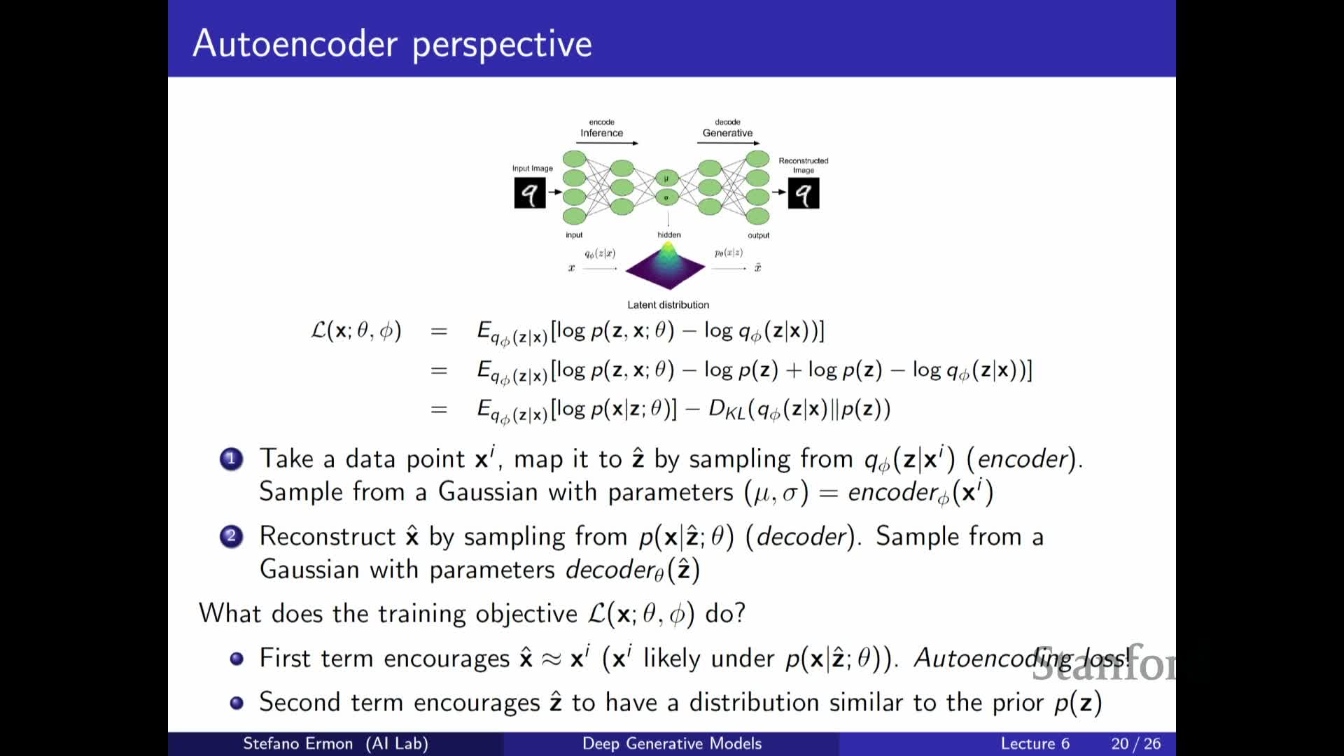
Rewriting the ELBO by adding and subtracting the prior p(z) makes the KL divergence explicit:
-
The regularizer appears as **KL[ q_φ(z x) p(z) ]** and pushes encoder outputs toward the chosen prior (commonly a standard Gaussian).
- Why this matters:
- The KL term encourages the marginal distribution of latent codes produced by the encoder to resemble the prior, so that sampling z ~ p(z) at generation time yields codes the decoder can meaningfully map to realistic x.
- The two ELBO terms therefore trade off reconstruction fidelity against conformity of inferred latents to the prior.
- Edge case:
-
When **q_φ(z x) = p_θ(z x)** (the true posterior), the ELBO equals the data log-likelihood, recovering maximum likelihood training.
-
Optimization choices and discrete latents: REINFORCE and encoder flexibility
When latent variables are discrete or the encoder choice makes reparameterization inapplicable, alternative gradient estimators are needed.
- General but higher-variance option:
-
REINFORCE and related score-function estimators provide a general route for optimizing the ELBO when reparameterization is not available.
-
REINFORCE and related score-function estimators provide a general route for optimizing the ELBO when reparameterization is not available.
- Encoder-family trade-offs:
- An overly restrictive q_φ increases the KL gap and hurts likelihood (underfitting the posterior).
- An overly flexible q_φ can better match the true posterior but may increase variance or require more computation.
- Determinism vs. stochasticity:
- The encoder may be made nearly deterministic if the true posterior is concentrated, but capturing posterior uncertainty typically requires stochastic encoders.
- The encoder may be made nearly deterministic if the true posterior is concentrated, but capturing posterior uncertainty typically requires stochastic encoders.
- Practical balancing act:
- Training balances encoder expressivity, estimator variance, and computational constraints.
- Alternative approaches (e.g., discriminator-based regularizers) can be used to align encoder marginals with priors when direct marginal matching is intractable.
Sampling at generation time and the role of the prior distribution
At generation time the encoder q_φ is not used; new samples are produced by sampling z from the fixed prior p(z) and decoding x ~ p_θ(x|z).
- Typical choices and caveats:
- The prior is often a simple distribution such as a standard Gaussian to enable easy sampling.
- The prior’s appropriateness depends on whether encoder posteriors and true posteriors are well-modeled by that family.
- Failure modes:
-
Posterior collapse: if **q_φ(z x)** collapses to the prior, the latent variables carry little information about x and generation becomes trivial but uninformative. -
Conversely, if **p(x z)** (the decoder) is overly powerful, the model can ignore z entirely.
-
- Design implications:
-
Choices for p(z), **p(x z), and **regularization strength determine whether the VAE produces meaningful latents and high-quality samples.
-
Autoencoding interpretation, compression, and mutual information trade-offs
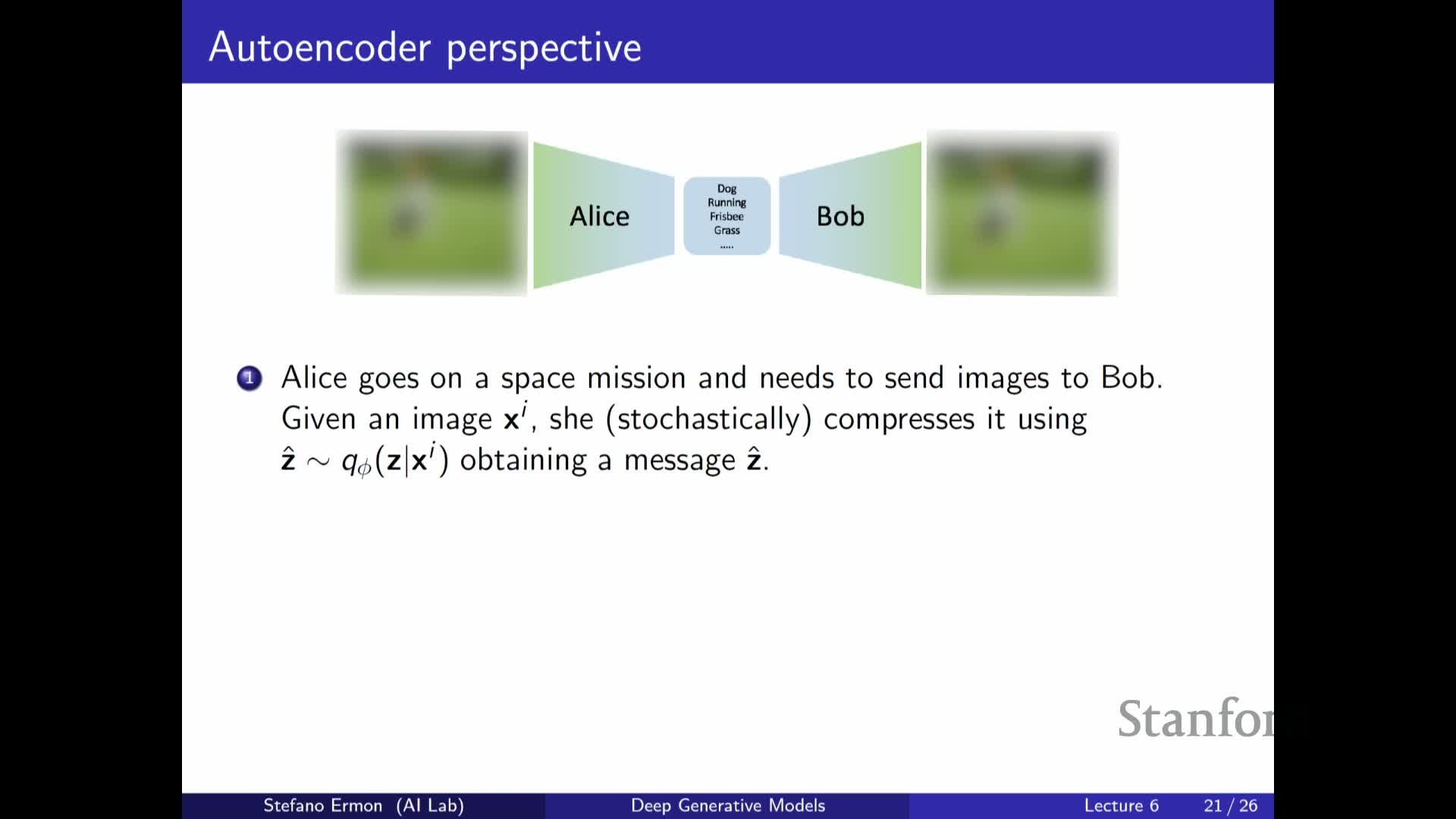
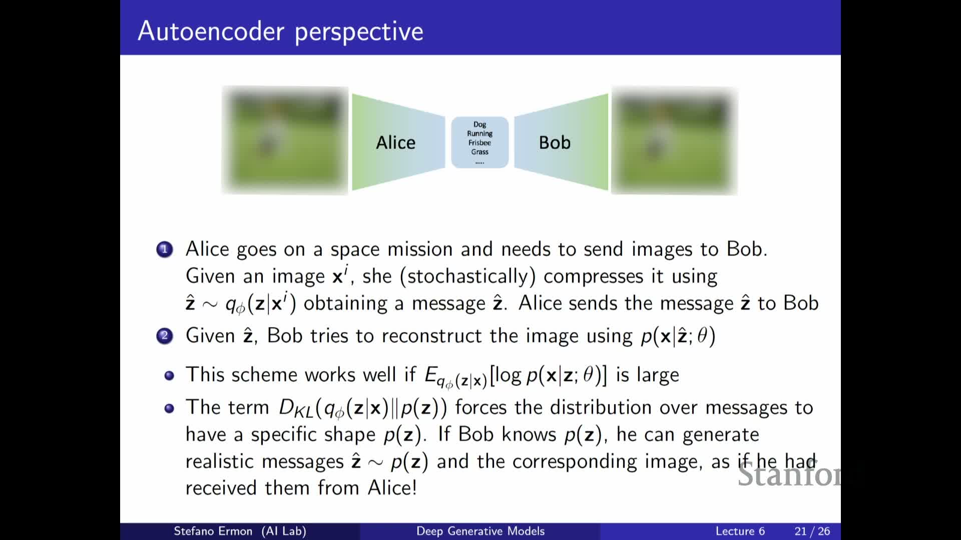
The ELBO reconceptualizes the VAE as a stochastic autoencoder that compresses an input x into a compact message z and decodes it back.
- Key perspective:
- The model trades off reconstruction quality against a constraint on the distribution of messages (via the KL term).
- The model trades off reconstruction quality against a constraint on the distribution of messages (via the KL term).
- Information-theoretic interpretation:
- The KL term controls mutual information between x and z: minimizing KL tends to reduce mutual information.
- This can be desirable for compression or privacy.
- It can be undesirable when informative latents are required for downstream tasks.
- The KL term controls mutual information between x and z: minimizing KL tends to reduce mutual information.
- Behavioral regimes:
- If the latent bottleneck is small or the KL penalty strong, the model clusters similar inputs together in latent space, performing lossy compression.
- If labels or task-specific objectives exist, they can be incorporated to steer latents toward semantically meaningful factors.
- Unifying view:
- This perspective unifies compression, feature discovery, and generative sampling under the ELBO objective.
- This perspective unifies compression, feature discovery, and generative sampling under the ELBO objective.
Practical considerations: computing the ELBO, sampling strategies, and synthetic augmentation
All components of the ELBO are computable in practice, with a few important remarks about tractability and variance.
- Closed-form pieces:
- The reconstruction likelihood and the KL between a Gaussian encoder and a Gaussian prior have closed-form expressions.
- The reconstruction likelihood and the KL between a Gaussian encoder and a Gaussian prior have closed-form expressions.
- Approximation and variance:
-
Remaining expectations are approximated by Monte Carlo sampling from **q_φ(z x)**. - Sampling multiple z per x reduces Monte Carlo variance and yields better gradient estimates, at increased computational cost.
- In practice, one or a few samples per minibatch are commonly used.
-
- Data augmentation caveat:
- Using synthetic samples from a trained generative model as augmented data is an active area, but naive augmentation can diverge under some assumptions.
- Theoretical and empirical care is required when mixing generated and real data.
- Practical summary:
- Training practice requires balancing computational budget, estimator variance, and dataset characteristics to achieve reliable encoder/decoder learning.
- Training practice requires balancing computational budget, estimator variance, and dataset characteristics to achieve reliable encoder/decoder learning.
VAE training dynamics: posterior collapse, reconstruction weight, and sample diversity
The ELBO’s reconstruction and KL terms naturally compete, and this competition can yield pathologies like posterior collapse if not managed.
- Collapse mechanisms:
-
Making the decoder too powerful or penalizing the KL too heavily can drive **q_φ(z x) ≈ p(z)** so latents are ignored.
-
- Remedies and techniques:
- Limit decoder capacity so the model must use z to reconstruct x.
- Anneal the KL term during training to gradually enforce prior matching.
- Encourage mutual information between x and z (e.g., auxiliary objectives) so latents capture meaningful variations.
- Sampling practice:
-
During training you must **sample from q_φ(z x)** (not just take the mode) to approximate the expectation and preserve multimodal posterior explanations. -
Multiple samples per x improve the fidelity of the estimate.
-
- Evaluation tip:
- Inspecting latent traversals by perturbing individual z dimensions helps diagnose whether axes encode interpretable factors of variation.
- Inspecting latent traversals by perturbing individual z dimensions helps diagnose whether axes encode interpretable factors of variation.
Flow models motivation: invertible latent-variable models with tractable likelihoods
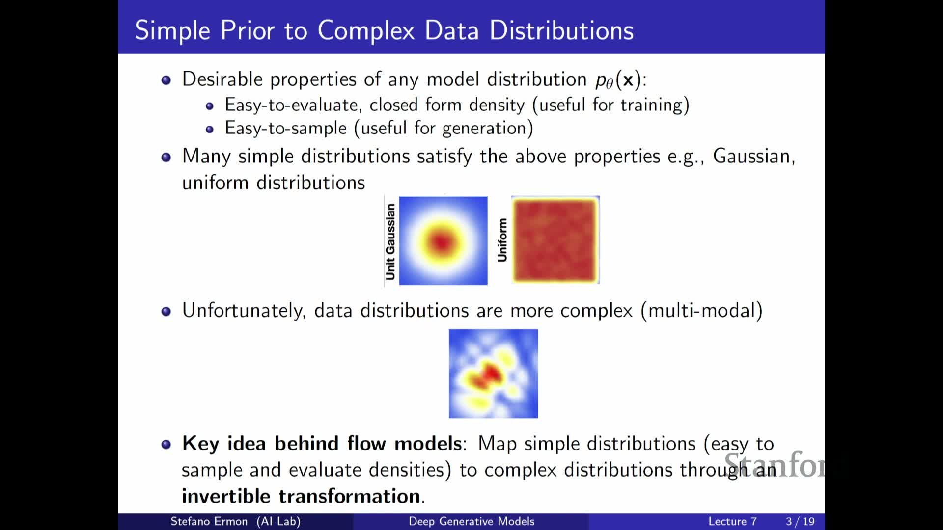
Flow models are introduced as an alternative latent-variable family that retains expressive marginal distributions while allowing exact density evaluation and sampling without variational inference.
- Core idea:
- Define x as a deterministic invertible transformation x = f(z) of a latent z drawn from a simple prior p(z).
-
Invertibility makes the mapping one-to-one so the marginal p(x) can be computed by a change of variables instead of an intractable integral.
- Practical consequences:
- This design removes the need for an encoder that integrates over multiple z values.
- Enables direct maximum likelihood training because each x corresponds to a unique z = f^{-1}(x).
- Trade-offs:
- Flow models forgo the compression advantage of VAEs in exchange for exact likelihoods and invertible mappings.
- Invertibility typically requires latent and data dimensions to match, which constrains architecture choices.
Change-of-variables in one dimension: CDF/PDF relationships and example transforms
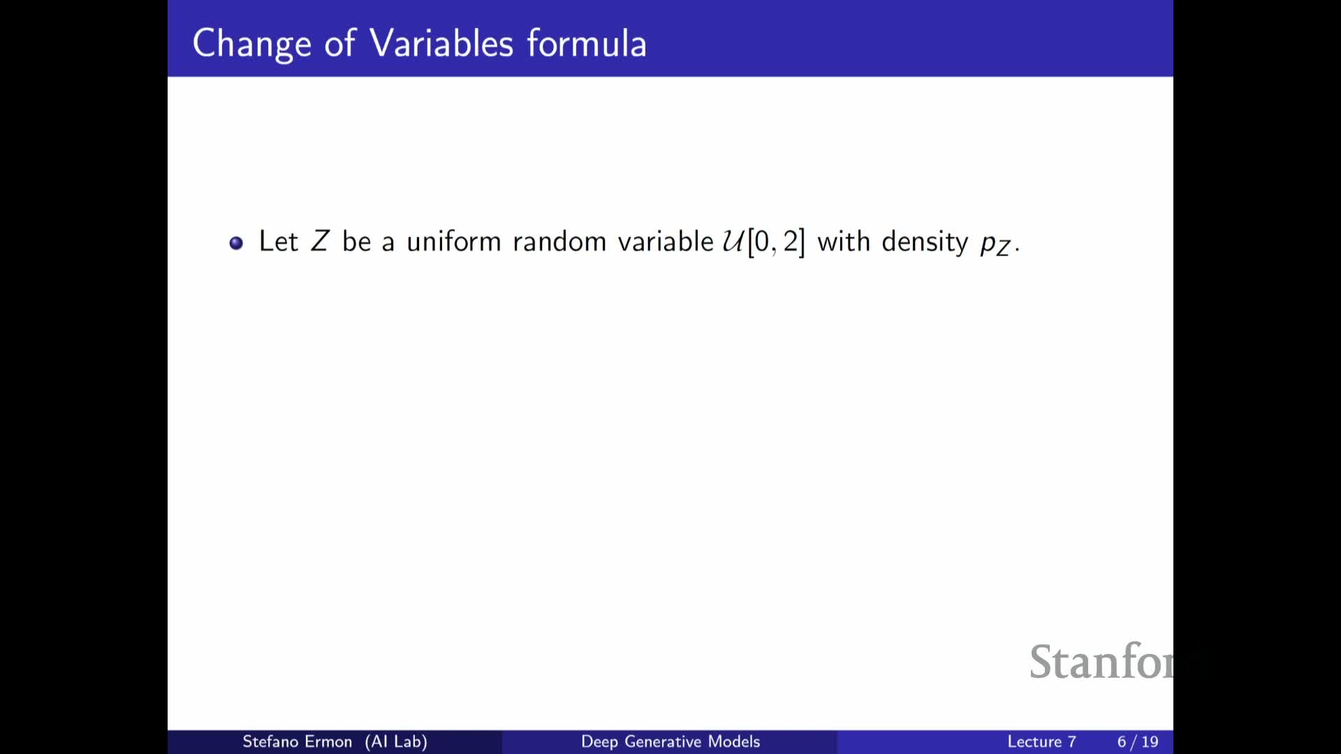
For a scalar invertible transform x = f(z) the output density follows the one-dimensional change-of-variables rule:
- Formula:
-
**p_X(x) = p_Z(f^{-1}(x)) * d/dx f^{-1}(x) **.
-
- Intuition and examples:
- The derivative factor comes from the relationship between CDFs and the chain rule and accounts for local stretching or compression of probability mass.
- Example: scaling z by a constant rescales the density by the inverse factor because support length changes.
- Example: exponentiation can map a uniform z into a heavy-tailed density p_X(x) ∝ 1/x on the transformed support.
- Generalization:
- The absolute derivative factor is essential to preserve normalization and the one-dimensional formula generalizes directly to higher dimensions via Jacobian determinants.
- The absolute derivative factor is essential to preserve normalization and the one-dimensional formula generalizes directly to higher dimensions via Jacobian determinants.
Linear multivariate transforms and the determinant of the Jacobian
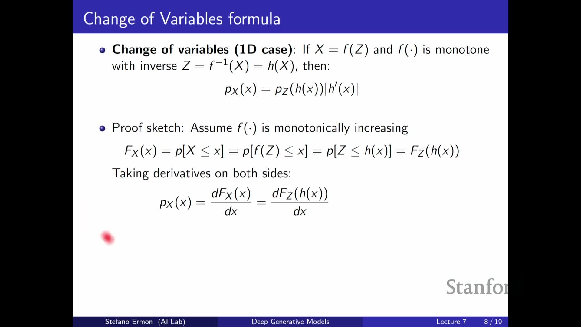
For vector-valued linear transforms x = A z the change-of-variables simplifies to a determinant-based scaling:
- Formula:
-
**p_X(x) = p_Z(A^{-1}x) * det(A^{-1}) **.
-
- Geometric interpretation:
-
The linear map A sends the unit hypercube to a parallelotope with volume det(A) . - The determinant encodes how the linear map stretches or shrinks volume in input space, providing the normalization factor so p_X integrates to one.
- When A is invertible, det(A^{-1}) = 1 / det(A) gives the appropriate density scaling.
-
- Motivation:
- This linear case motivates the multivariate nonlinear formula where the Jacobian determinant of the invertible mapping generalizes linear determinants.
- This linear case motivates the multivariate nonlinear formula where the Jacobian determinant of the invertible mapping generalizes linear determinants.
Nonlinear invertible mappings and the multivariate change-of-variables formula
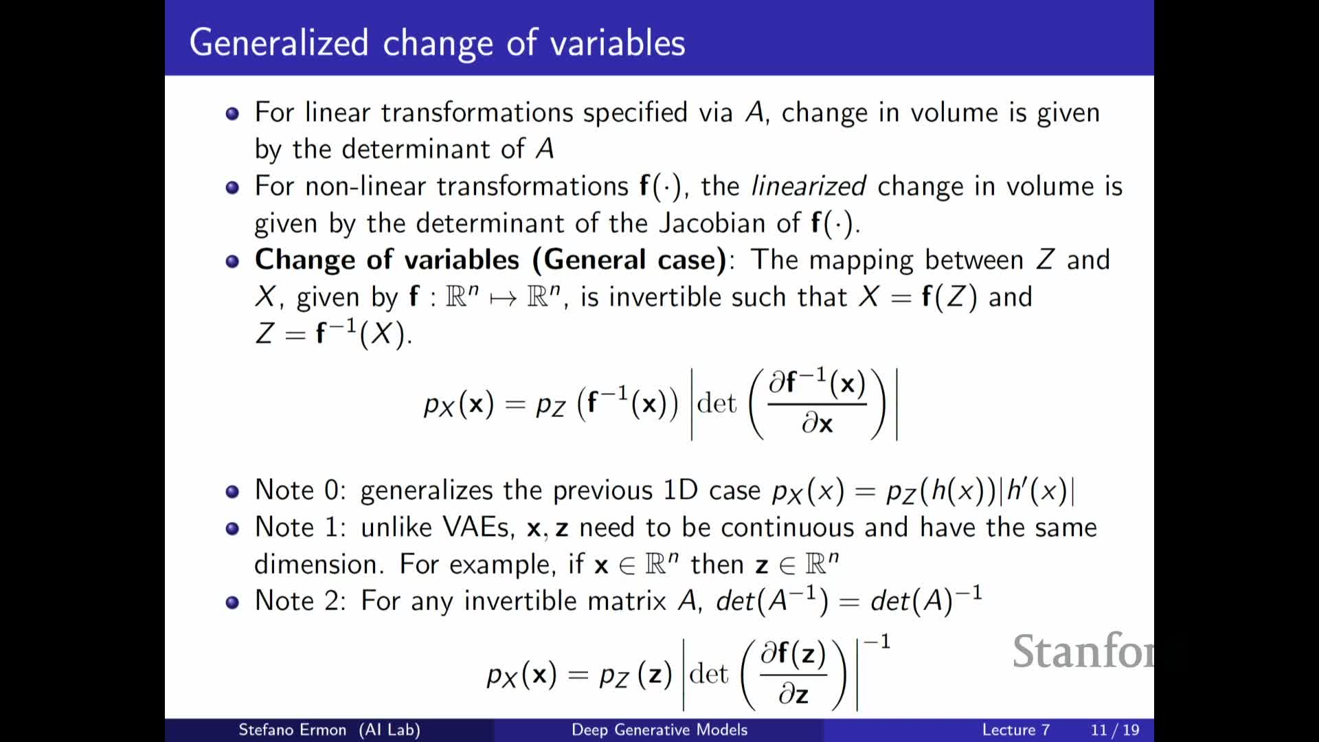
When f is an invertible smooth mapping between equal-dimensional Euclidean spaces, the multivariate change-of-variables formula is:
- Equivalent forms:
-
**p_X(x) = p_Z(f^{-1}(x)) * det(J_{f^{-1}}(x)) ** -
Equivalently **p_X(x) = p_Z(z) * det(J_f(z)) ^{-1}**, with z = f^{-1}(x).
-
- Notation and meaning:
- J denotes the Jacobian matrix of partial derivatives.
- The determinant of the Jacobian measures local volume change under the nonlinear map and supplies the normalization correction.
- Practical implications for flow design:
- Flow models require architectures where the inverse mapping and the Jacobian determinant are tractable to compute, or where the Jacobian can be arranged to factorize or be efficiently evaluated.
- Designing neural network layers with cheap invertibility and manageable Jacobian-determinant computation is the central engineering challenge of normalizing flows.
- Different flow families trade off expressivity and computational tractability accordingly.
Enjoy Reading This Article?
Here are some more articles you might like to read next: