Stanford CS236- Deep Generative Models I 2023 I Lecture 8 - Normalizing Flows
- Normalizing flows define deterministic invertible latent-variable models that allow exact likelihood evaluation
- Exact likelihoods for flows are computed by the change-of-variables formula including the Jacobian determinant
- Flows permit exact likelihoods without variational approximations but require equal input and latent dimensionality
- Composing simple invertible layers yields flexible normalizing flows
- Architectural design must guarantee invertibility and efficient determinant/inverse computation
- Planar and low-dimensional visualizations illustrate how flows warp simple priors into complex densities
- Maximum-likelihood training for flows uses exact likelihoods computed by inversion and Jacobian determinants
- Triangular Jacobian structure and autoregressive ordering yield linear-time determinant computation
- Additive coupling layers (NICE) partition variables and apply simple, invertible updates with unit Jacobian
- Volume-preserving coupling plus simple rescaling can produce useful image models but has limitations
- RealNVP extends additive coupling by combining shift and scale to obtain expressive, non-volume-preserving layers
- Latent interpolations and empirical behavior show flows learn meaningful one-to-one representations
- Autoregressive models are a special case of flows: continuous conditionals correspond to sequential shift-and-scale transforms
- Inverse autoregressive flows (IAF) trade off fast sampling for expensive inversion, enabling single-shot generation
- Teacher-student distillation leverages flows to obtain fast samplers from autoregressive teachers (Parallel WaveNet example)
- Flows operate on continuous densities; masked convolutional/invertible convolutions extend flow design to images
- Gaussianization and CDF-based transforms provide an alternative perspective on flows by iteratively mapping data to a simple prior
Normalizing flows define deterministic invertible latent-variable models that allow exact likelihood evaluation
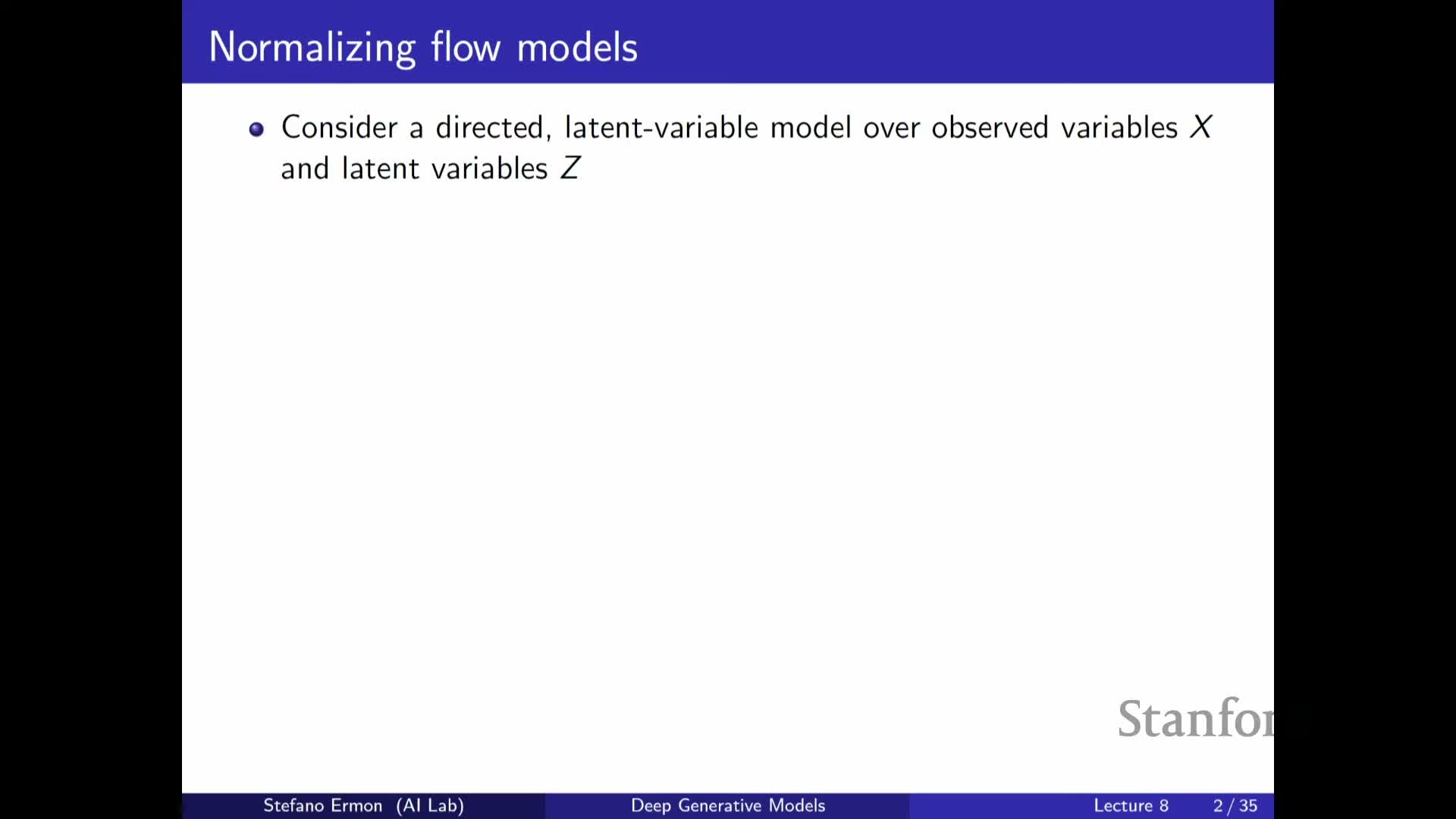
A normalizing flow is a latent-variable model that maps simple latent variables Z to observed variables X using a deterministic, invertible mapping F_Θ.
The mapping is parameterized (typically by neural networks).
Because the mapping is invertible, inference of Z given X reduces to applying the inverse mapping F_Θ⁻¹, and likelihoods can be computed exactly rather than approximated with variational encoders—combining expressive generative modeling with tractable likelihood computation suitable for maximum-likelihood training.
Exact likelihoods for flows are computed by the change-of-variables formula including the Jacobian determinant
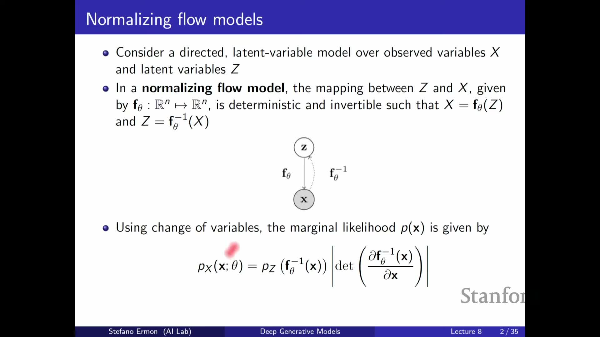
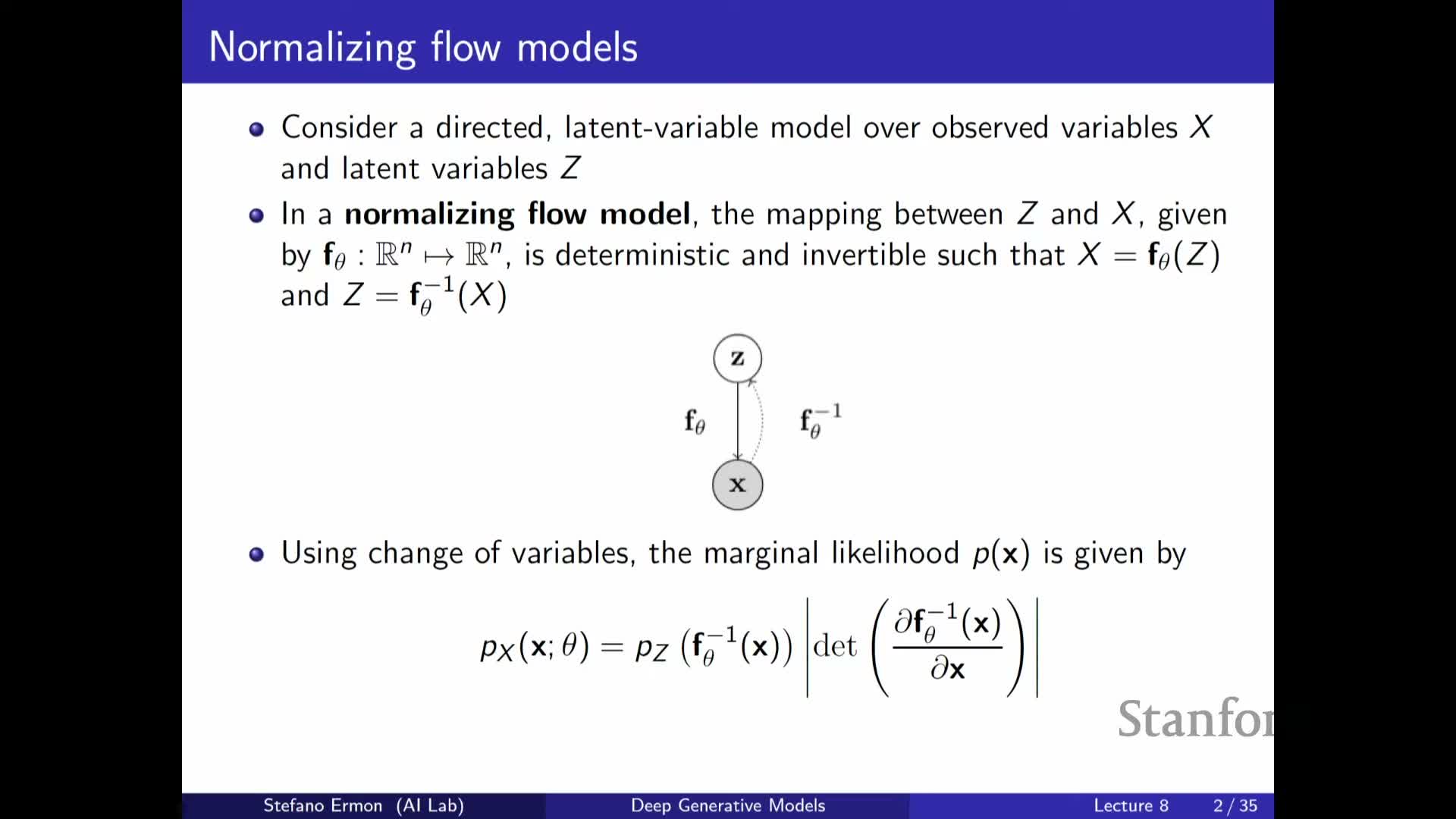
The probability density for an observed x under a flow is
-
p_X(x) = p_Z(z) det(dz/dx) , where z = F_Θ⁻¹(x) and dz/dx is the Jacobian of the inverse mapping.
Intuitively:
- The prior probability of the corresponding latent z is adjusted by the local expansion or contraction of volume encoded by the determinant of the Jacobian.
- Computing that determinant accurately is essential to produce a normalized density that integrates to one.
In practice the determinant is handled via structural constraints on layers or algebraic manipulations that make evaluation tractable.
Flows permit exact likelihoods without variational approximations but require equal input and latent dimensionality
Normalizing flows avoid variational approximations because inference is exact when the mapping is invertible and the Jacobian determinant is computable.
A necessary modeling constraint is that the latent vector Z and data X must have the same dimensionality for the mapping to be bijective.
This contrasts with VAEs, where the latent dimension can be lower than the data dimension and compression is explicit. The equal-dimension requirement therefore:
- Shapes architectural choices (you must design bijective primitives), and
- Influences downstream use of the latent space: the latent is a one-to-one representation rather than a compressed encoding.
Composing simple invertible layers yields flexible normalizing flows
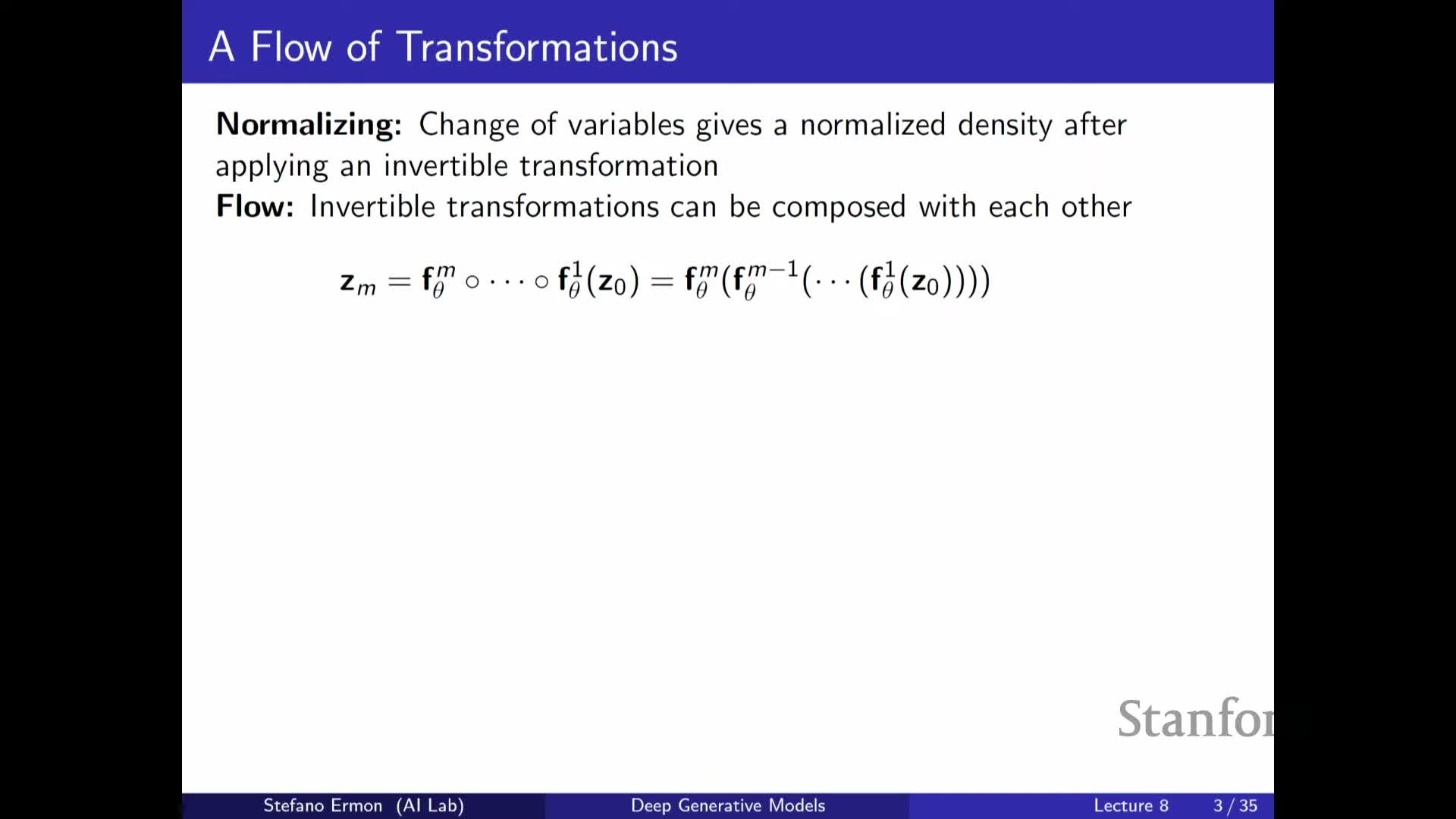
Normalizing flows build complex mappings by composing multiple simple invertible layers f₁, f₂, …, f_M parameterized by neural networks.
Key points:
- If each layer is invertible then the composition is invertible.
- The overall Jacobian determinant equals the product of per-layer determinants, so architectures focus on layer primitives that are:
- Individually invertible,
-
Efficiently invertible, and
- Yield tractable determinants.
- Individually invertible,
- Stacking many simple layers produces expressive transformations analogous to deep networks built from simple blocks.
Architectural design must guarantee invertibility and efficient determinant/inverse computation

Practical flow design requires three operational properties:
-
Guaranteed invertibility for all parameter settings.
-
Efficient computation of the inverse mapping.
-
Tractable evaluation of the Jacobian determinant.
Naively computing determinants of general n×n Jacobians costs O(n³) and is prohibitive for high-dimensional data.
Standard engineering solutions:
- Constrain layer computations so the Jacobian has special structure (e.g., triangular, diagonal, or low-rank modifications) that permit linear- or near-linear-time determinant computation.
- Choose architectures so inversion can be computed analytically or via cheap iterative schemes.
Planar and low-dimensional visualizations illustrate how flows warp simple priors into complex densities
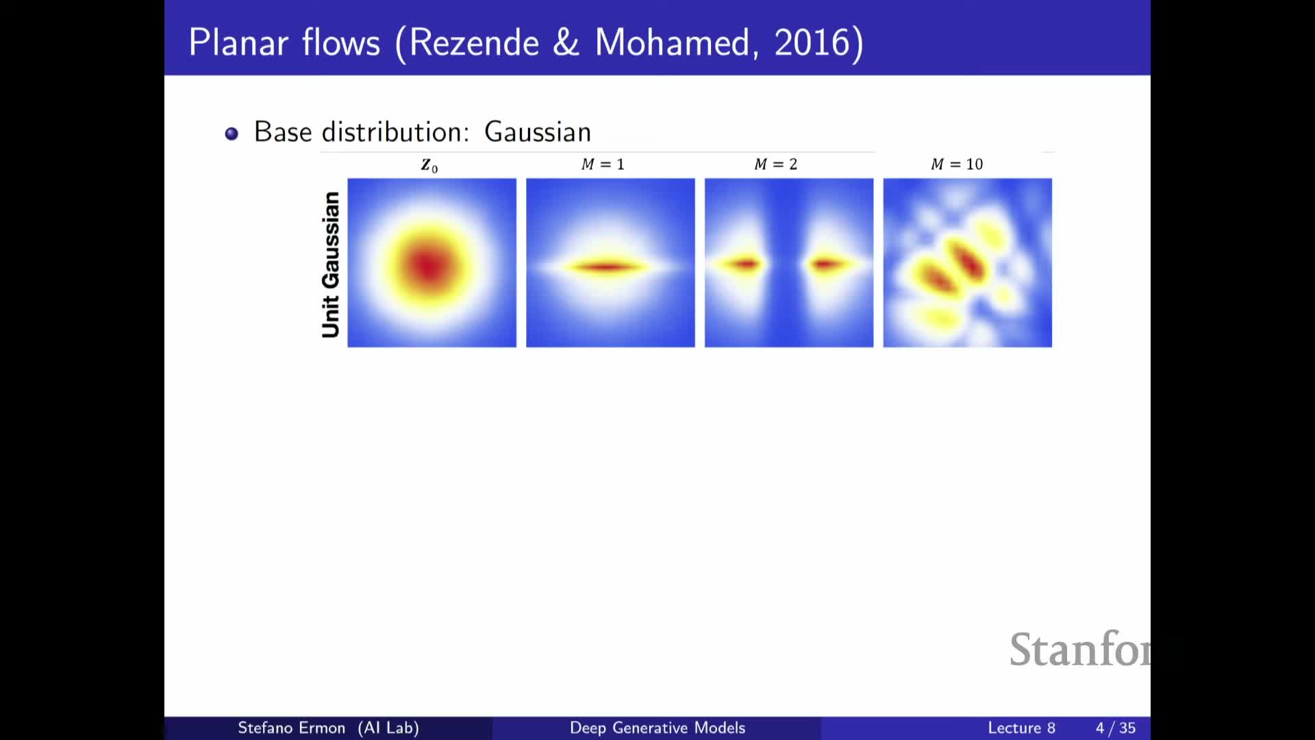
Flows can be visualized in 2D where successive invertible layers warp an initial simple prior (e.g., spherical Gaussian or uniform square) into progressively more complex densities.
Visualization insights:
- Each layer applies a local deformation that redistributes probability mass.
- Repeated composition enables multi-modal and highly structured target densities.
- These examples show how expressive distributions arise from simple primitives by iterative remapping and provide intuition for deep flow design in higher dimensions.
- They underscore that even simple layer formulas can produce complex global transformations when stacked.
Maximum-likelihood training for flows uses exact likelihoods computed by inversion and Jacobian determinants
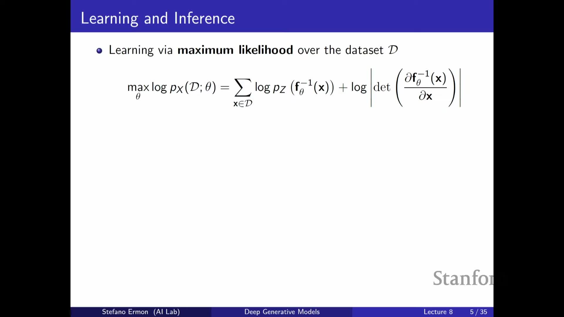
Flows are trained by maximizing the average log-likelihood of training data, which is computable via:
- Inversion of each x to z using F_Θ⁻¹.
- Evaluation of the prior density p_Z(z).
- Addition of the log-determinant term from the change-of-variables formula.
Because both terms are explicit given a tractable inverse and determinant, gradients with respect to parameters Θ can be computed and standard gradient-based optimization applied.
This direct likelihood training mirrors autoregressive and other exact-likelihood approaches and avoids variational ELBO approximations—the optimization target places probability mass near observed data by tuning the sequence of invertible layers.
Triangular Jacobian structure and autoregressive ordering yield linear-time determinant computation
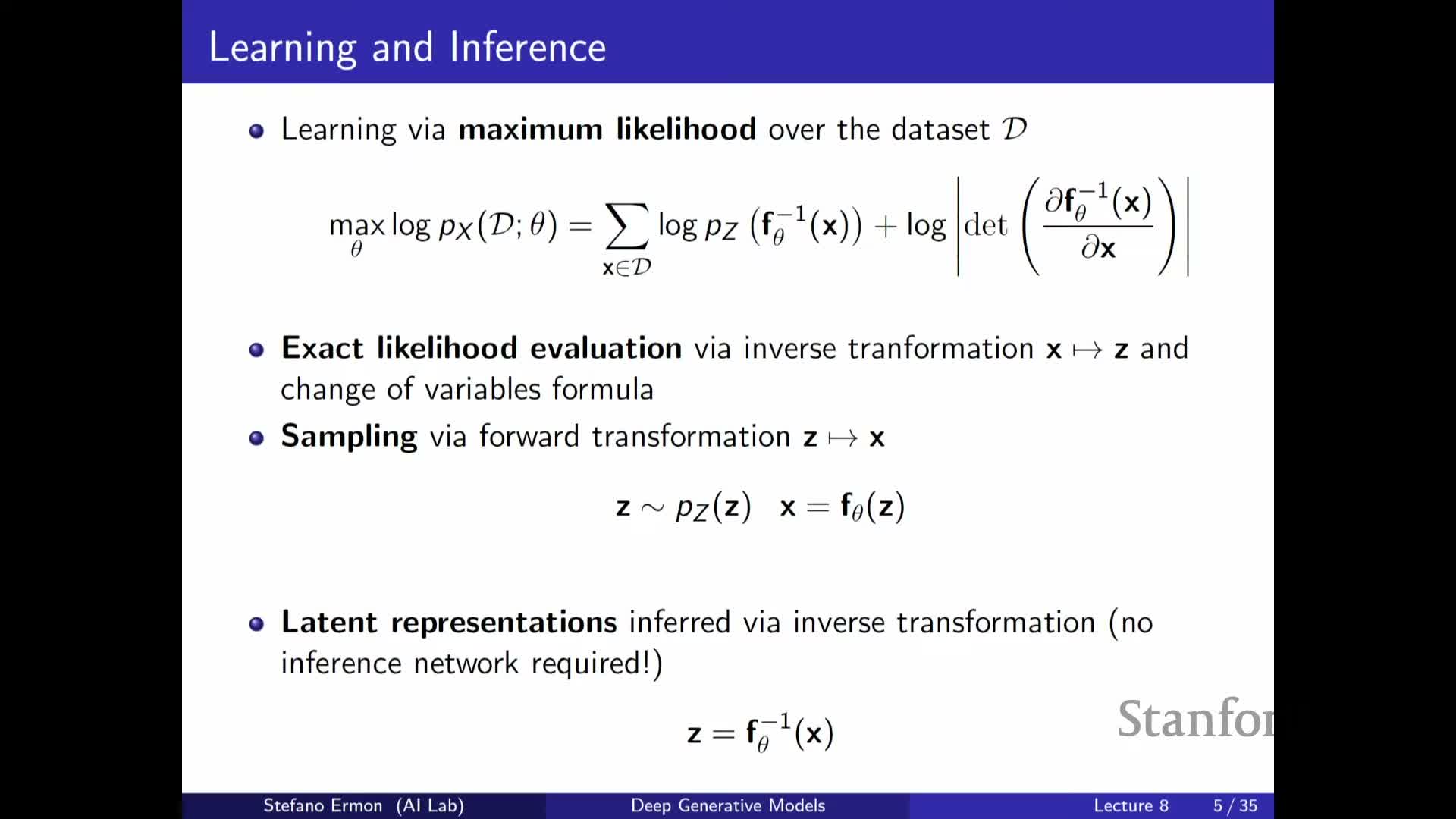
One effective way to make Jacobian determinants cheap is to design layers whose Jacobians are triangular under some ordering of variables.
Mechanism and consequence:
- If each output dimension depends only on a subset of input dimensions (e.g., only previous inputs in an ordering), many off-diagonal partials are zero and the Jacobian becomes triangular.
- The determinant of a triangular matrix equals the product of diagonal entries, allowing O(n) determinant evaluation.
- This insight motivates architectures that impose computational graphs similar to autoregressive models or masked convolutions to achieve tractable determinants.
Additive coupling layers (NICE) partition variables and apply simple, invertible updates with unit Jacobian
An additive coupling layer (as used in NICE) splits the input into two subsets x₁ and x₂, leaves x₁ unchanged, and replaces x₂ by x₂ + m_Θ(x₁) where m_Θ is an arbitrary neural network.
Properties:
- The forward mapping is trivially invertible because x₁ is copied and x₂ is recovered by subtraction.
- The Jacobian is block-triangular with an identity diagonal, so its determinant equals one.
- Such layers are volume-preserving and the coupling network m_Θ can be arbitrarily flexible while preserving invertibility and cheap inversion.
- Stacking many coupling layers with different partitions yields expressive but computationally tractable flows.
Volume-preserving coupling plus simple rescaling can produce useful image models but has limitations
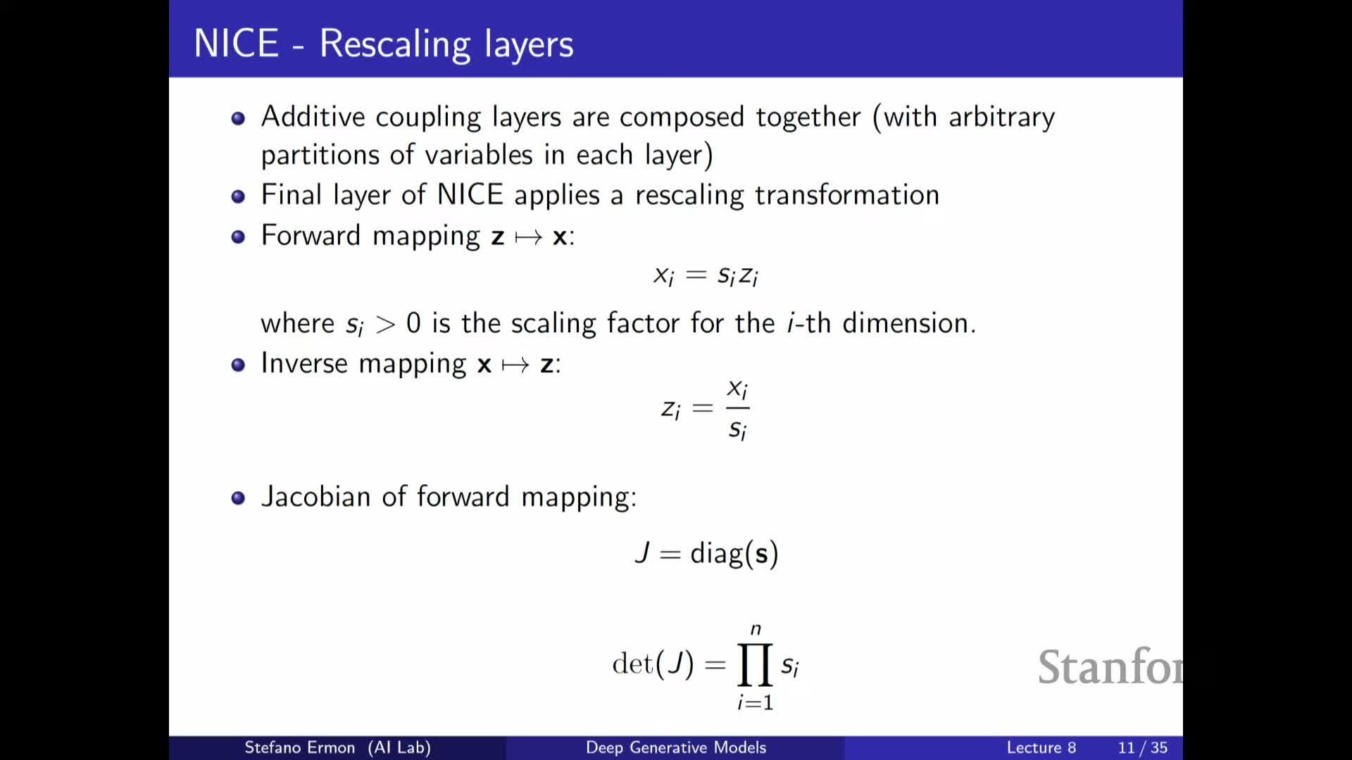
Volume-preserving coupling layers can be supplemented by learnable elementwise rescaling factors to introduce non-volume-preserving transforms and enable the model to expand or contract volume along coordinates.
Notes:
- The rescaling layer outputs a diagonal Jacobian with determinant equal to the product of scale factors, which is cheap to compute and invertible provided scales are nonzero.
- Empirically, stacks of coupling and rescaling layers (with permuted partitions between layers) can model image datasets like MNIST, SVHN, and CIFAR-10 and produce plausible samples, though sample quality may lag state-of-the-art generative models.
- These designs demonstrate that relatively simple primitives, stacked sufficiently deep, yield practical density estimators.
RealNVP extends additive coupling by combining shift and scale to obtain expressive, non-volume-preserving layers
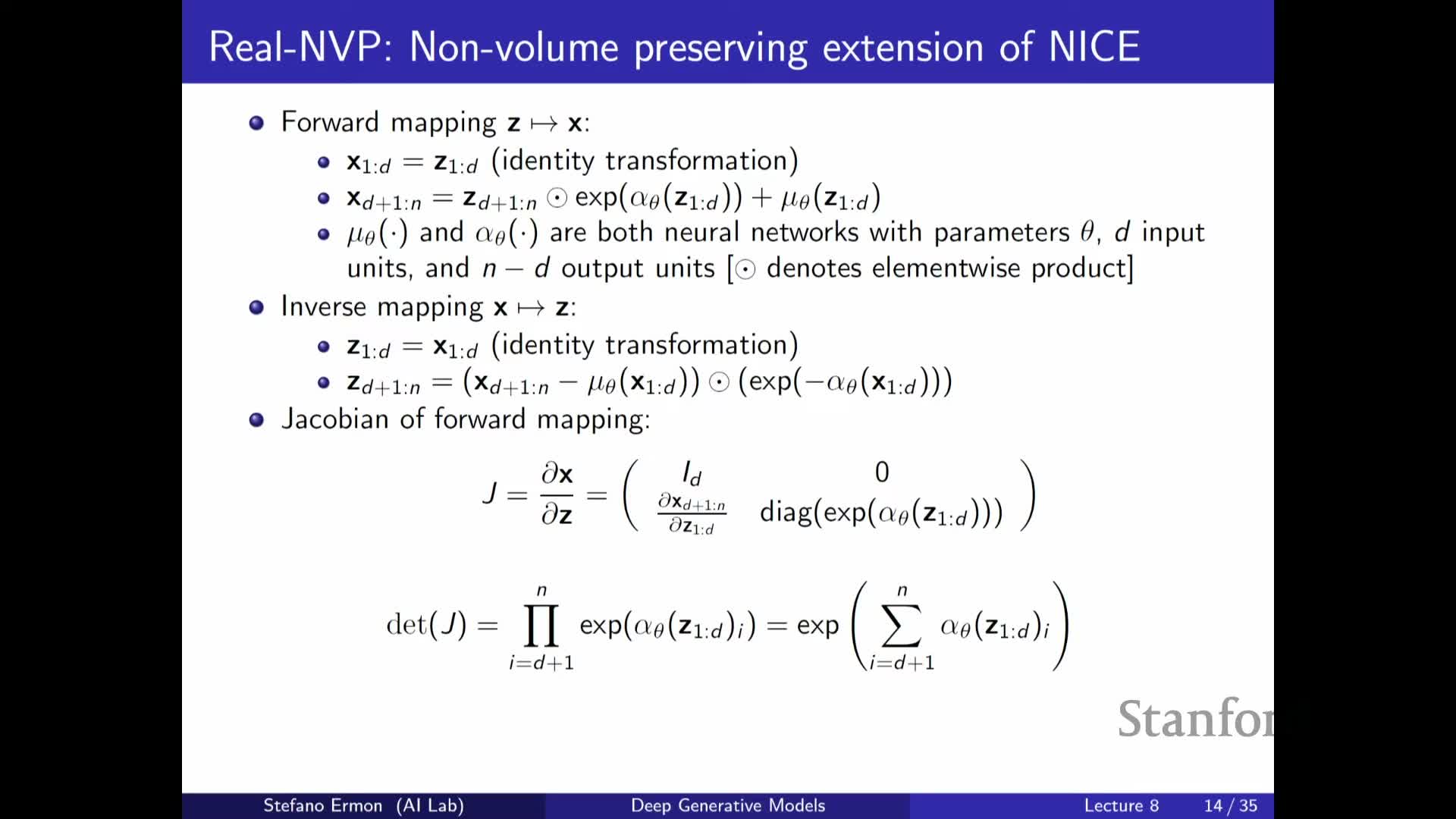
RealNVP coupling layers generalize additive coupling by applying both an additive shift μ_Θ(x₁) and an elementwise scale exp(α_Θ(x₁)) to the second partition:
- x₂’ = (x₂ + μ_Θ(x₁)) * exp(α_Θ(x₁)).
Properties:
- The mapping remains trivially invertible because x₁ is preserved and x₂ is recovered by subtracting μ_Θ and dividing by the scale.
- The Jacobian is lower-triangular with diagonal entries equal to the exponentiated scaling factors, so the log-determinant reduces to a sum of α_Θ outputs.
- Allowing learned scaling factors makes the layer strictly more flexible than volume-preserving coupling layers.
Latent interpolations and empirical behavior show flows learn meaningful one-to-one representations
Although flow latents have the same dimensionality as data and are therefore not compressive in the VAE sense, flow-trained latent spaces exhibit structure meaningful for tasks such as interpolation.
How interpolation is used:
- Map real data to latent Z via inversion.
- Interpolate in Z-space (e.g., along geodesics or linearly after appropriate normalization).
- Decode back to data space to obtain smooth transitions.
Empirical results show plausible interpolation trajectories for faces and scenes, indicating flows learn semantically useful coordinate systems despite bijectivity, supporting flows for representation tasks where invertibility and smoothness are valued.
Autoregressive models are a special case of flows: continuous conditionals correspond to sequential shift-and-scale transforms
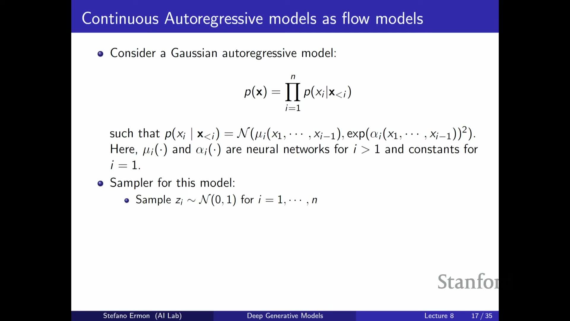
A continuous autoregressive model with Gaussian conditionals can be represented as a flow by treating independent standard normals z_i as base noise and mapping them sequentially with shift-and-scale transforms whose parameters depend on previous outputs.
Key equivalences:
- Sampling the autoregressive model (z -> x) corresponds to shifting and scaling z_i using means and variances predicted from earlier x values, matching the functional form of coupling or affine transforms.
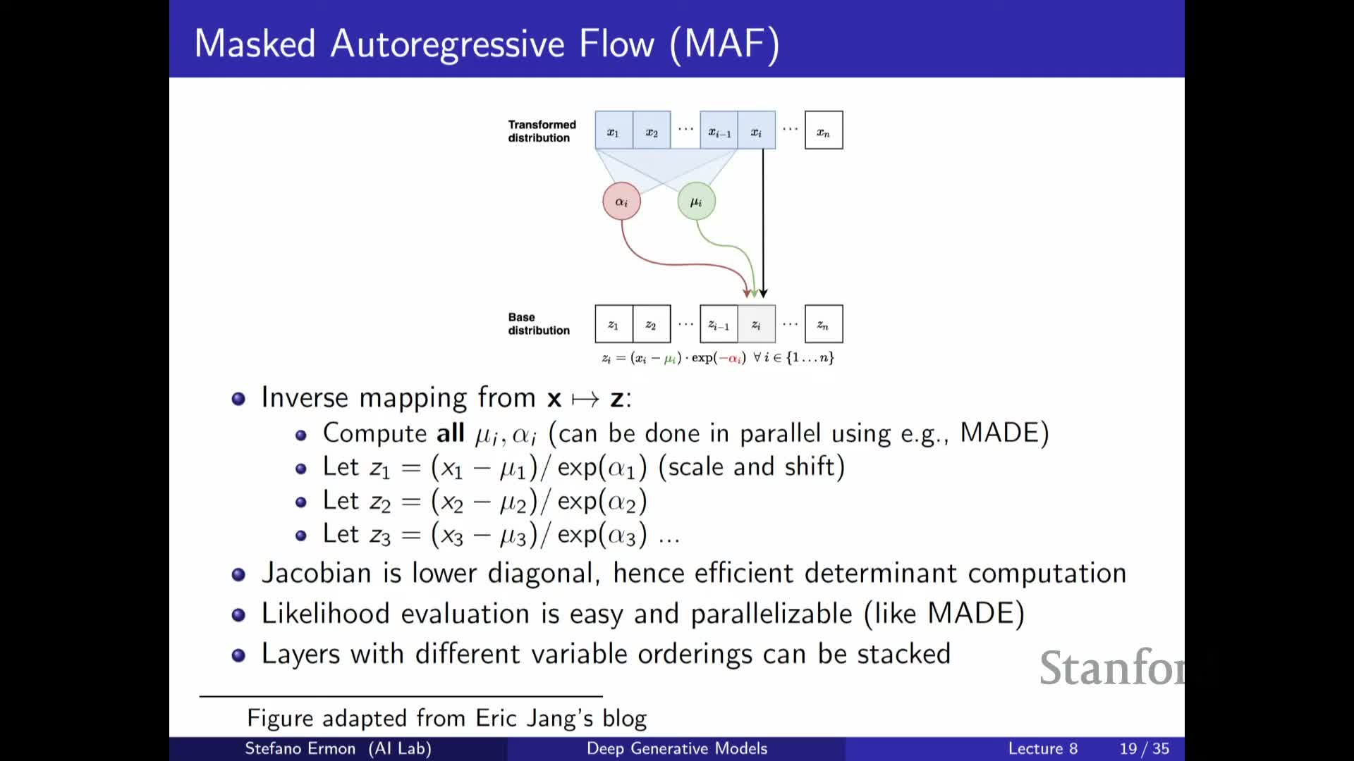
- From the likelihood perspective, inverting the mapping (x -> z) can be done in parallel because all conditionals’ parameters are computable from the observed x.
- Thus autoregressive models inherit the flow property and the same triangular Jacobian structure for tractable determinant computation.
Inverse autoregressive flows (IAF) trade off fast sampling for expensive inversion, enabling single-shot generation
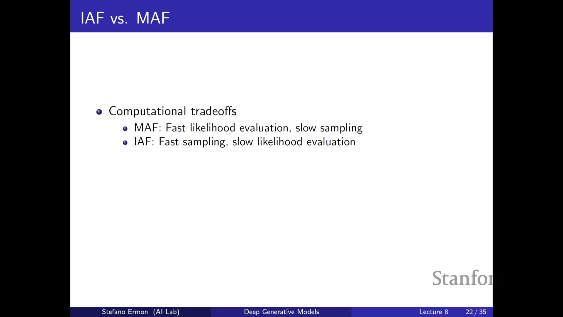
By swapping roles of x and z in an autoregressive flow one obtains an inverse autoregressive flow (IAF) where the forward direction z->x is parallel and hence allows single-step sampling of the entire output.
Trade-offs:
- Benefit: fast generation (parallel sampling).
- Cost: inversion (x->z) becomes sequential because each inversion step requires previously recovered latents, making likelihood evaluation expensive at training time.
Conversely, masked autoregressive flows (MAF) are the opposite: efficient likelihoods, slow sampling. The two families are duals under variable relabeling and their trade-offs guide use cases.
Teacher-student distillation leverages flows to obtain fast samplers from autoregressive teachers (Parallel WaveNet example)
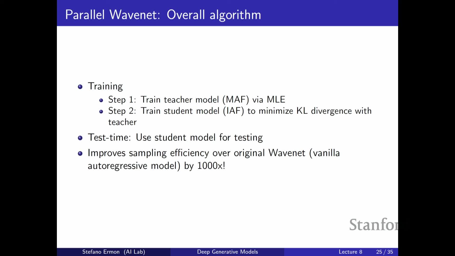
A practical pipeline distills a high-quality autoregressive teacher trained by maximum likelihood into a fast-sampling student IAF by minimizing KL(student || teacher).
Typical distillation steps:
- Train a high-quality autoregressive teacher (maximum-likelihood).
-
Train a student IAF to minimize KL(student teacher), which requires: - Sampling from the student, and
- Evaluating teacher likelihoods of those samples.
- Sampling from the student, and
- The student must be easy to sample from and able to evaluate its own sample densities efficiently (true for invertible student models when student latent codes are known).
This distillation yields fast generation models that approximate teacher behavior (e.g., used in Parallel WaveNet for speech generation).
Flows operate on continuous densities; masked convolutional/invertible convolutions extend flow design to images
Normalizing flows apply to continuous probability densities and are not directly applicable to discrete data such as token sequences because the change-of-variables formula requires a continuous domain.
For image modeling:
- Flow layers can be implemented with masked or specially constrained convolutions so that the resulting Jacobian is triangular and invertible, enabling efficient determinant computation.
- Masking enforces an ordering over pixels and channels similar to PixelCNN-style autoregressive masks, giving invertible convolutional primitives that preserve tractable density computation.
- Such convolutional flow layers can be stacked to model high-dimensional image distributions while exploiting locality.
Gaussianization and CDF-based transforms provide an alternative perspective on flows by iteratively mapping data to a simple prior

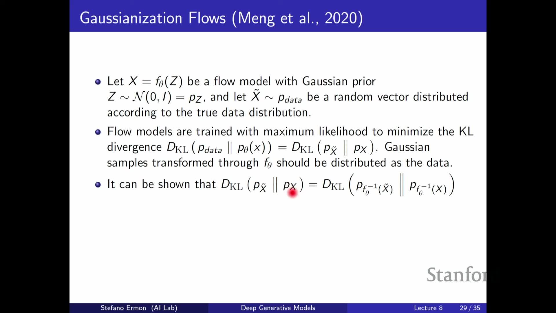
Training a flow to maximize likelihood can be viewed equivalently as transforming data through the inverse mapping toward a simple prior such as a standard Gaussian.
One-dimensional intuition:
- The probability integral transform maps a variable’s CDF to a uniform random variable, and composing with the inverse Gaussian CDF maps it to Gaussian marginals.
Practical perspective:
-
Gaussianization layers apply marginal transforms and simple rotations or couplings iteratively to make the joint distribution increasingly Gaussian.
- This connects flows to classical statistical techniques (e.g., copulas, marginal transforms) and motivates layers that progressively “whiten” the data distribution.
Enjoy Reading This Article?
Here are some more articles you might like to read next: