Stanford CS236- Deep Generative Models I 2023 I Lecture 9 - GANs
- Generative modeling framework and common model families
- Maximum likelihood as a principled training objective
- High likelihood need not imply good sample quality and vice versa
- Two-sample testing as an alternative criterion for distribution similarity
- A learned classifier (discriminator) can implement a powerful two-sample test statistic
- GANs formulate generator and discriminator learning as a minimax game and connect to Jensen–Shannon divergence
- Practical training challenges: instability, oscillations, and mode collapse
- GAN ideas remain valuable and can be integrated with other generative approaches
Generative modeling framework and common model families
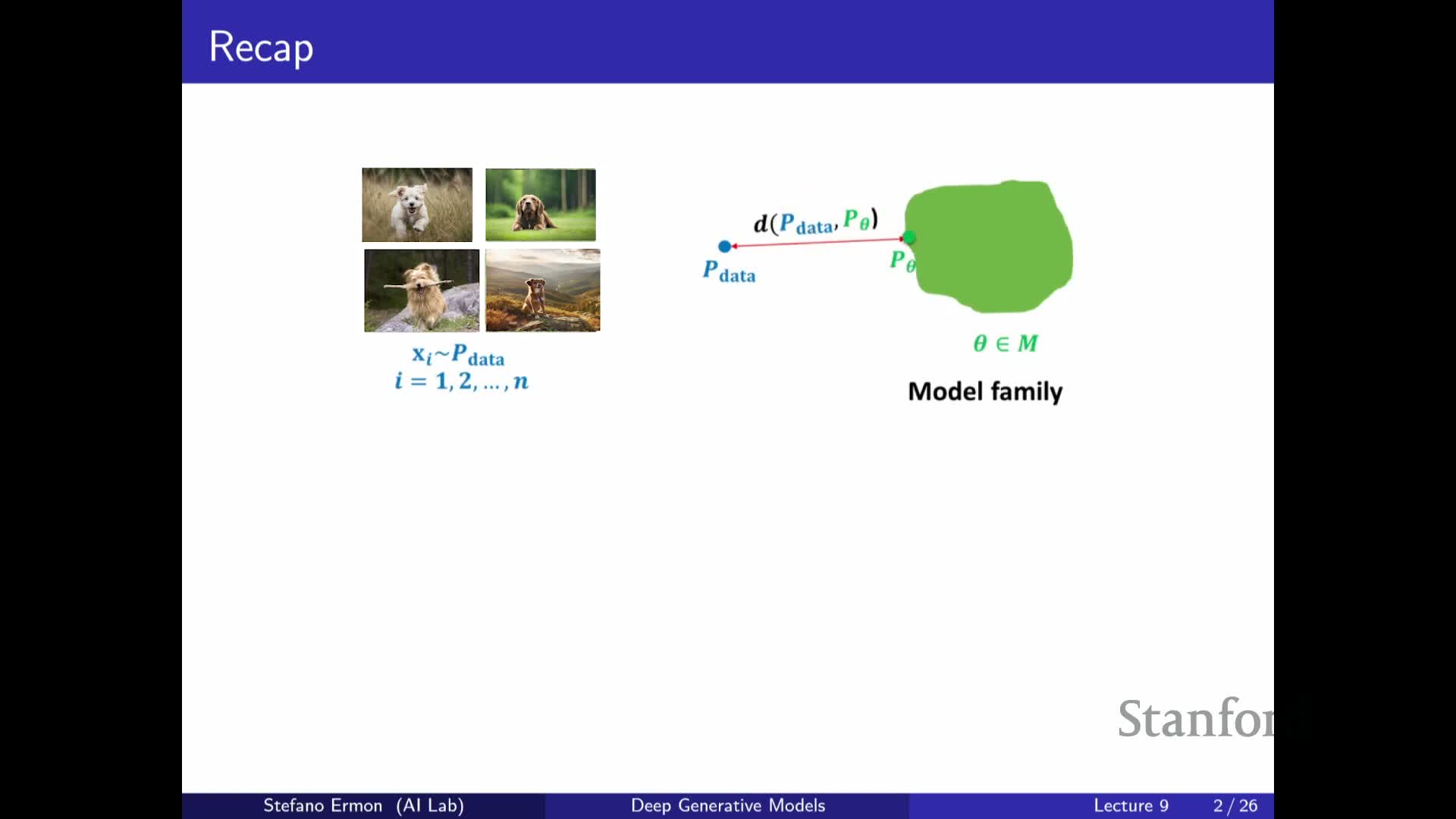
Generative modeling treats the dataset as independent and identically distributed (i.i.d.) samples from an unknown data distribution and defines a parametric model family of probability distributions, typically instantiated by neural networks.
Common model families include:
-
Autoregressive models — factorize the joint distribution via the chain rule.
-
Variational autoencoders (VAEs) — approximate densities through latent-variable mixtures.
-
Normalizing flows — obtain exact densities via invertible deterministic transformations and the change-of-variables formula.
The typical training paradigm is a two-step process:
- Define a similarity measure between the data distribution and a candidate model distribution.
- Search the parameter space for the model that minimizes that similarity metric.
A central design constraint is choosing a representation and training objective that permit efficient evaluation of model probability for any data point — this requirement strongly shapes architecture and optimization choices.
Maximum likelihood as a principled training objective
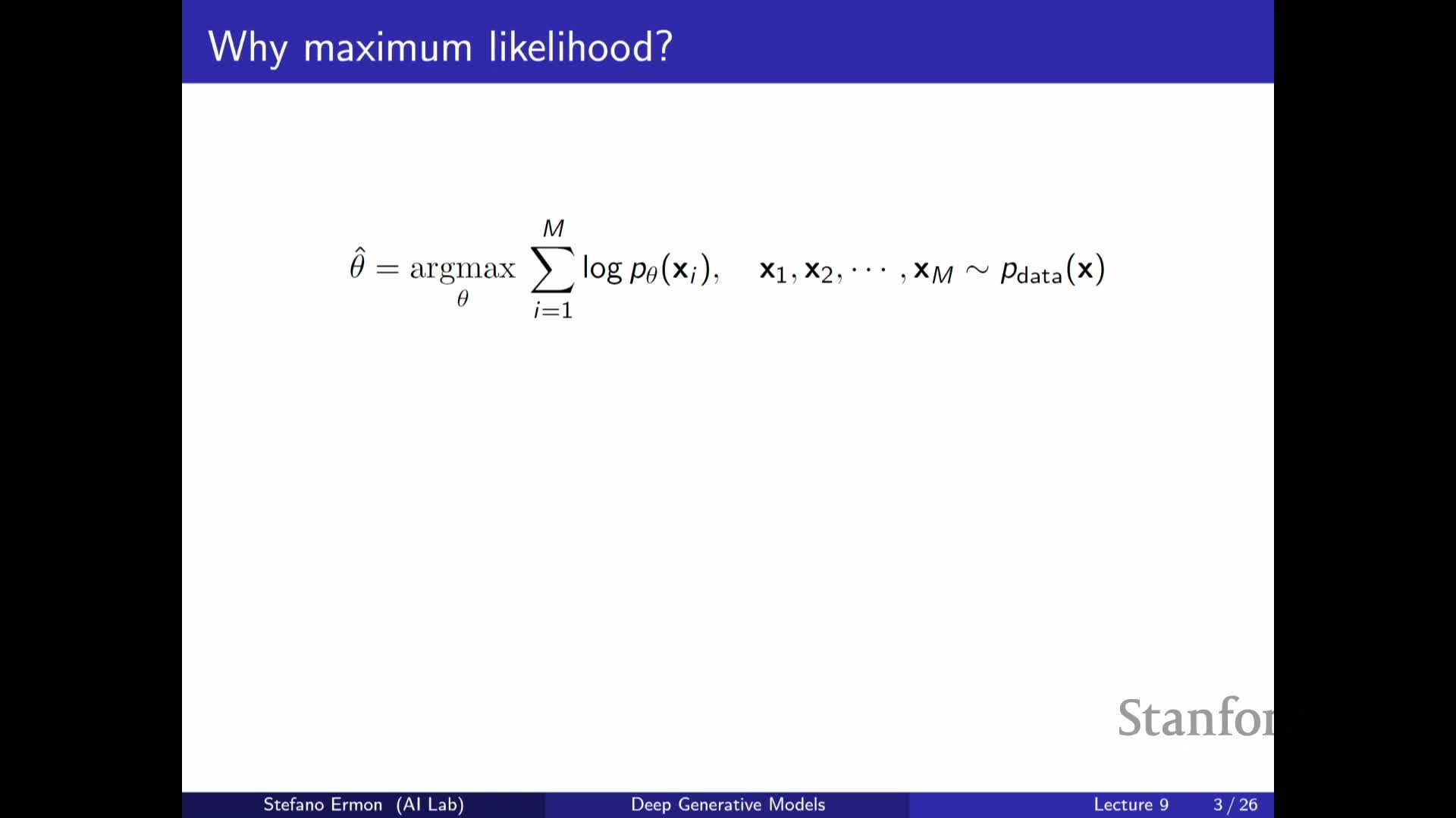
Maximum likelihood training optimizes model parameters to maximize the probability assigned to observed data — equivalently, it minimizes the Kullback–Leibler (KL) divergence from the data distribution to the model.
Key practical and theoretical points:
- It requires the ability to evaluate the model density or mass function for given inputs.
- The resulting single-sample objective is the average log-probability, which can be optimized with stochastic gradients.
- Under standard regularity assumptions and sufficient model capacity, maximum likelihood estimators are statistically efficient — they converge faster and use data more effectively than many alternatives.
- There is an information-theoretic view: high likelihood corresponds to good compression of the data, so likelihood optimization encourages representations that capture true structure rather than noise.
High likelihood need not imply good sample quality and vice versa
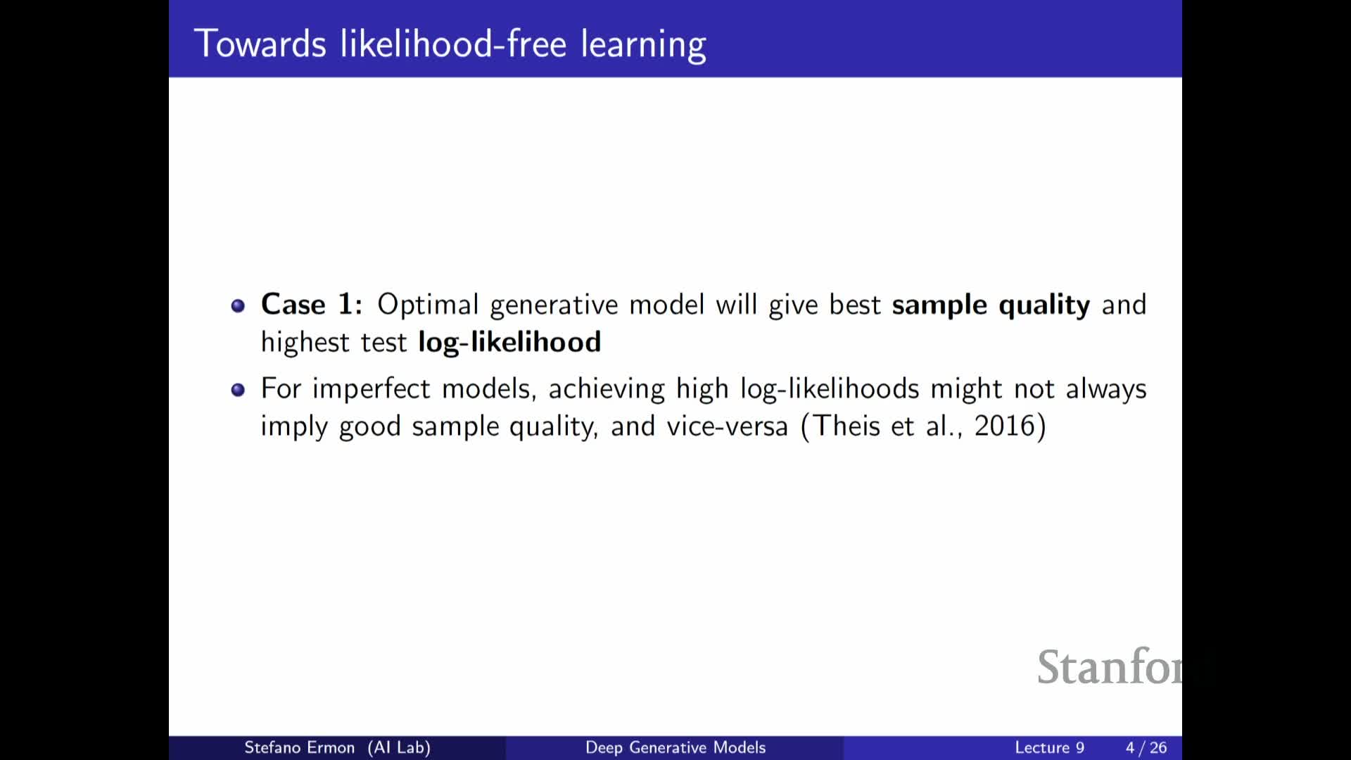
Likelihood and perceptual sample quality can diverge. A model can attain very good average log-likelihood yet produce mostly poor samples, and conversely can generate visually realistic samples while assigning low likelihood to held-out data.
A canonical failure-mode construction:
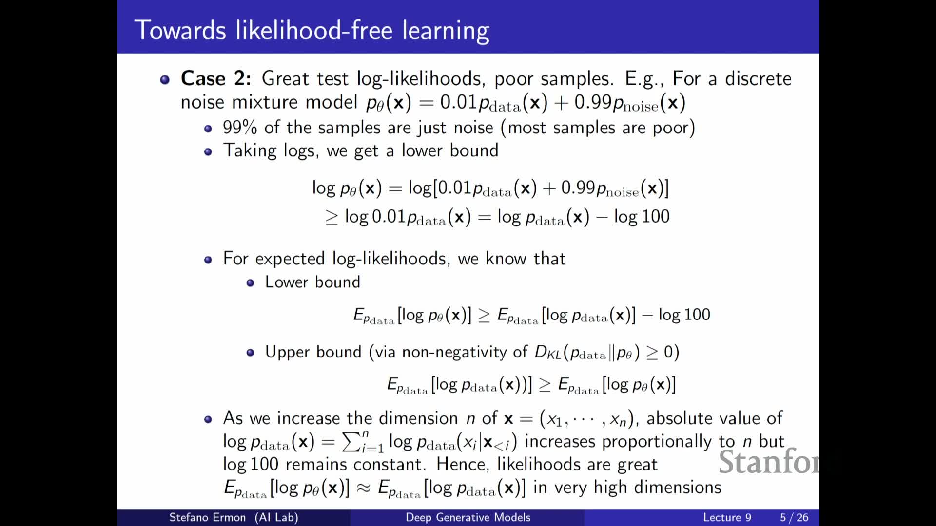
- Build a mixture that outputs true data with a small probability (e.g., 1%) and random garbage otherwise.
- The model’s log-probability on true data is shifted by a constant (the log of the mixing weight), so the average likelihood can remain high even though most generated samples are garbage.
Additional factors that widen the gap:
- In high-dimensional settings the linear scaling of log-likelihood with dimensionality makes constant shifts negligible, further decoupling likelihood from sample fidelity.
-
Overfitting gives the opposite failure: concentrating mass on the finite training set can produce perfect-looking samples but catastrophic generalization likelihoods.
These observations motivate alternative training criteria that focus directly on sample quality rather than relying solely on likelihood.
Two-sample testing as an alternative criterion for distribution similarity
Two-sample tests ask whether two sets of samples come from the same distribution by computing a test statistic on the samples and running a hypothesis test.
Practical considerations:
- Simple handcrafted statistics include differences of empirical means or variances.
- In high dimensions many distributions can match low-order statistics yet differ in other important ways, so designing a discriminative and general statistic is challenging.
- Two-sample tests expose the tradeoffs of Type I and Type II errors: finite-sample randomness forces thresholds and accept/reject error rates, and test power depends on the chosen statistic.
A major advantage is that sample-based tests do not require model likelihoods, enabling training objectives that rely only on drawing samples from candidate models.
A learned classifier (discriminator) can implement a powerful two-sample test statistic
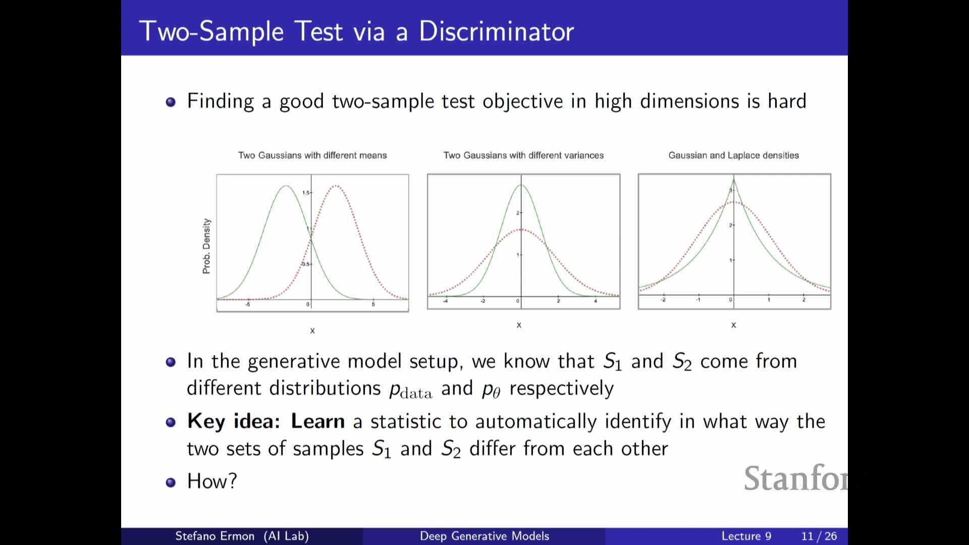
A parameterized binary classifier trained to discriminate real data from model-generated samples serves as a learned two-sample test statistic.
How it works:
- The classifier is trained with a cross-entropy objective to output high probability on real samples and low probability on fake ones.
- The negative classification loss (or the classifier’s accuracy) is a statistic that grows when the two distributions are more distinguishable.
- Crucially, this statistic depends only on samples and the classifier’s likelihood over the binary label — not on the model density over data — so it imposes no requirement that the generator provide tractable likelihoods and allows arbitrarily expressive, sampleable generators.
- When the classifier cannot distinguish the two sample sets beyond chance, that provides evidence that the generator distribution approximates the data distribution.
GANs formulate generator and discriminator learning as a minimax game and connect to Jensen–Shannon divergence
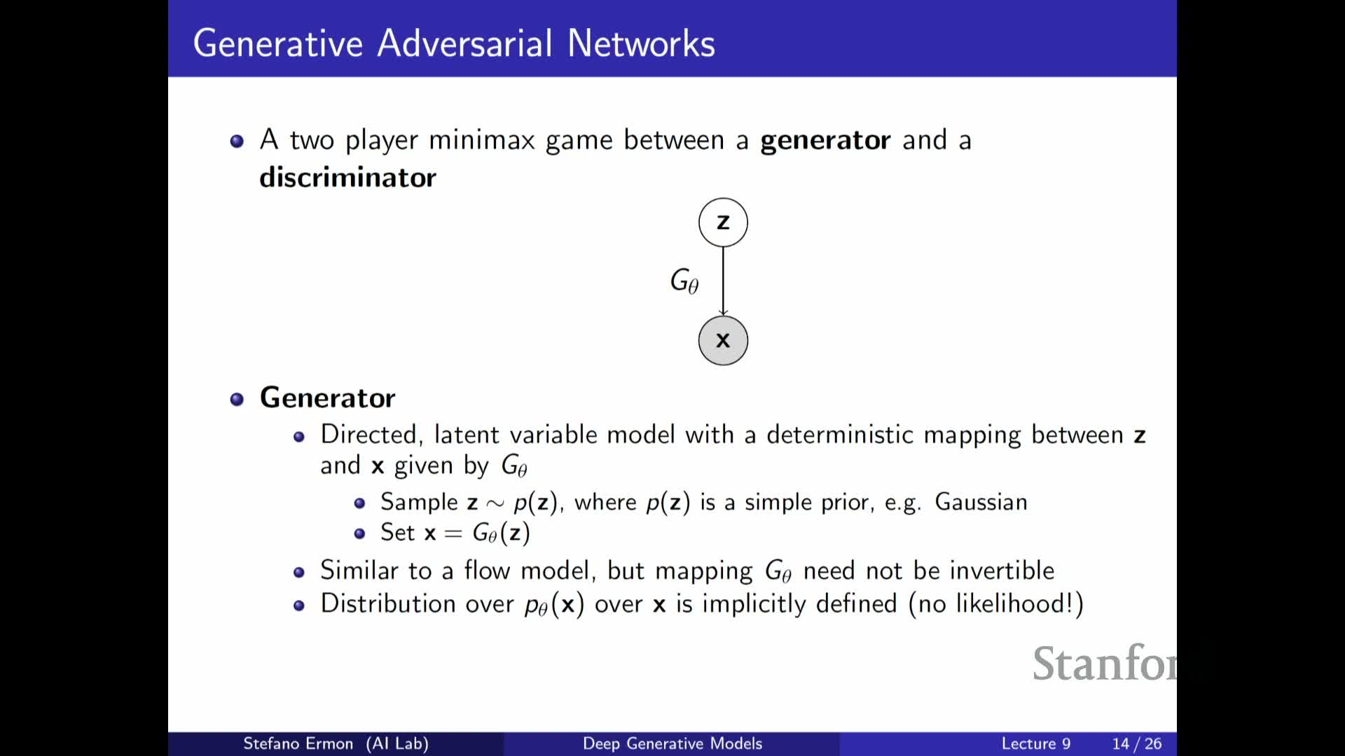
Generative adversarial training frames learning as a two-player minimax optimization between a discriminator and a generator.
Viewed as a process:
- The discriminator maximizes its ability to distinguish real from generated samples by minimizing classification loss on the binary task.
- The generator updates its parameters to minimize that same objective — i.e., to produce samples that fool the discriminator.
Theoretical properties:
- For a fixed generator, the optimal discriminator outputs the posterior proportional to the density ratio pdata / (pdata + pmodel).
- Substituting this optimal discriminator into the adversarial objective yields an expression equal to a constant plus twice the Jensen–Shannon divergence between the data and model distributions, so the global minimizer of the minimax game matches the data distribution.
A key practical advantage is that this formulation requires only sampling from the generator and evaluating discriminator outputs, not computing model likelihoods or invertible mappings.
Practical training challenges: instability, oscillations, and mode collapse
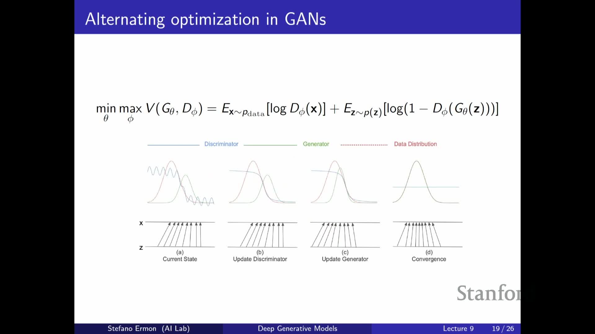
In practice, adversarial minimax optimization is often unstable.
Common practical issues:
- Alternating gradient updates for discriminator and generator frequently produce nonconvergent oscillations, making loss curves unreliable as progress indicators.
-
Mode collapse is a frequent failure mode: the generator becomes mode-seeking and concentrates mass on a small subset of data modes rather than covering the full distribution — a behavior contrasting with maximum-likelihood objectives, which heavily penalize missing modes.
Mitigation requires many empirical techniques and architectural choices, for example:
-
Regularization
-
Noise injection
- Carefully tuned training schedules
-
Ensemble methods and other heuristics
None of these guarantees convergence, and these practical difficulties are a major reason many practitioners have shifted toward diffusion-based generative models, which present a single, more stable optimization objective and more predictable training behavior.
GAN ideas remain valuable and can be integrated with other generative approaches
Despite these training difficulties, adversarial ideas remain valuable as a mechanism for learned, sample-based comparison and can be combined with other generative frameworks to improve sample fidelity.
Typical ways adversarial components are used:
- Incorporate discriminators into diffusion or likelihood-based models to refine perceptual quality.
- Use GAN-style generators to permit highly flexible, noninvertible mappings from latent space to data space.
- Initialize or combine generators with pretrained latent-variable models or VAEs, though common practice often trains generators from scratch on large datasets.
Historical milestones — for example, early GAN-generated artworks — illustrate both the creative potential and cultural impact of adversarial generative models, even as research attention shifts toward methods with more stable optimization properties.
Enjoy Reading This Article?
Here are some more articles you might like to read next: