Stanford CS236- Deep Generative Models I 2023 I Lecture 10 - GANs
- Generative Adversarial Networks train implicit generative models via a minimax game between a generator and a discriminator
- F-divergences generalize KL by scoring density ratios with a convex scalar function
- Direct evaluation of f-divergences is infeasible in likelihood-free settings because density ratios require access to probabilities under data or model distributions
- The convex conjugate (Fenchel conjugate) provides a variational representation that moves f applied to a density ratio into a supremum over linear terms involving that ratio
- Parametrizing the supremum witness by a neural network yields a sample-based lower bound on the f-divergence and a discriminator training objective
- F-GAN formulates a practical minimax objective that approximately minimizes a chosen f-divergence by alternating discriminator and generator updates
- The Wasserstein (Earth Mover) distance measures distribution mismatch via optimal transport and remains meaningful when supports are disjoint
- The Kantorovich–Rubinstein dual expresses Wasserstein-1 as a supremum over 1-Lipschitz witness functions, enabling a GAN-style critic when Lipschitzness is enforced
- Wasserstein-GAN objectives mitigate vanishing gradients and training instability common with JS/KL-based GANs but require careful enforcement of the Lipschitz constraint
- Bi-directional GAN variants introduce an encoder to infer latent variables by training a discriminator on joint (data,latent) pairs
Generative Adversarial Networks train implicit generative models via a minimax game between a generator and a discriminator
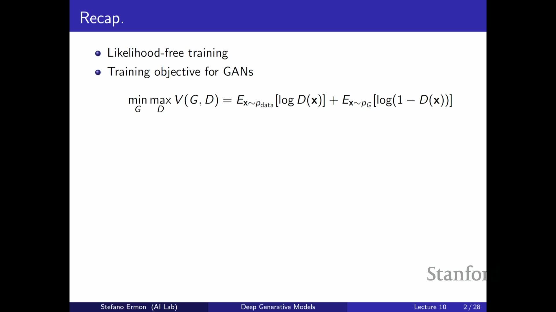
Generative Adversarial Networks (GANs) frame generative modeling as a two-player minimax optimization: a generator maps samples from a simple prior to model samples, while a discriminator performs binary classification between real and generated samples.
- The discriminator is trained to maximize classification accuracy (equivalently minimize negative cross-entropy).
- The generator is trained to minimize the discriminator’s ability to distinguish real from fake, producing a saddle-point objective.
Under an optimal discriminator assumption, the generator’s objective corresponds to minimizing a divergence between the data distribution and the model distribution; in the original formulation this reduces (up to scale and shift) to the Jensen–Shannon divergence.
Because the generator can be an implicit model that only requires sampling (not likelihood evaluation), GANs enable flexible architectures that avoid explicit density factorization or tractable probability evaluation.
F-divergences generalize KL by scoring density ratios with a convex scalar function
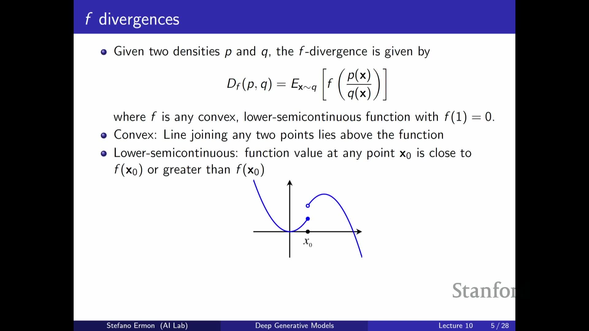
An f-divergence defines a family of discrepancy measures between two distributions P and Q by taking an expectation under Q of a convex scalar function f applied to the density ratio u(x) = p(x)/q(x): D_f(P||Q) = E_{x~Q}[ f(u(x)) ].
Key properties of f: it must be convex, lower semi-continuous, and satisfy f(1) = 0, which ensures non-negativity of the divergence and zero value iff P = Q under mild conditions.
Common examples (choices of f) include:
- f(u) = u log u → Kullback–Leibler (KL) divergence
- f(u) = −log u → reverse KL
- A symmetric choice of f → Jensen–Shannon divergence
- Other choices → squared Hellinger, total variation, etc.
The f-divergence family therefore provides a flexible framework for penalizing different kinds of discrepancies between distributions by changing the shape of f.
Direct evaluation of f-divergences is infeasible in likelihood-free settings because density ratios require access to probabilities under data or model distributions
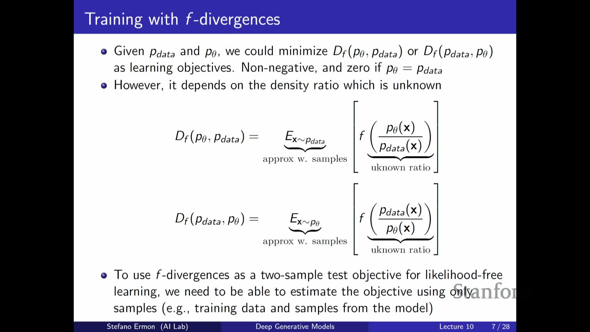
The definition of f-divergences depends on density ratios p(x)/q(x), which requires evaluating either the model density q(x) or the data density p(x).
- In practical likelihood-free scenarios the data density p_data is unknown and implicit models do not provide tractable q(x), so the divergence cannot be computed directly.
- While sample averages can approximate expectations when the expectation measure is accessible via samples, the dependence on the density ratio inside f prevents straightforward sample-only optimization.
Therefore a reformulation is required that expresses the f-divergence (or a bound thereof) in terms of expectations that only require sampling from P and Q.
The subsequent variational reformulation uses convex duality to move the dependence on the density ratio into a linear term that can be estimated by a classifier-like function.
The convex conjugate (Fenchel conjugate) provides a variational representation that moves f applied to a density ratio into a supremum over linear terms involving that ratio
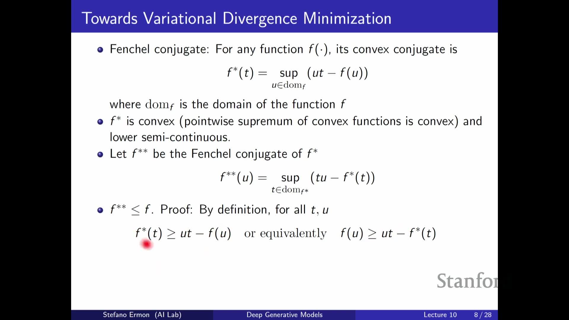
Given a scalar convex function f, its convex (Fenchel) conjugate f* is defined by f*(t) = sup_{u} (u t − f(u)).
Useful properties:
- f* is convex in t.
- The biconjugate f** is a lower bound to f, with equality when f is convex and lower semi-continuous.
Applying this pointwise to f evaluated at the density ratio u(x) = p(x)/q(x) yields the identity
f(u(x)) = f(u(x)) = sup_{t} (t u(x) − f*(t)), which converts the nonlinear dependence on u(x) into a **linear dependence on u(x) under an outer supremum.
Substituting this into the expectation under Q and simplifying produces a difference of two expectations — one under P and one under Q — making the expression amenable to sample-based estimation and inviting the introduction of a parametrized witness function t(x) (a discriminator) to approximate the supremum.
Parametrizing the supremum witness by a neural network yields a sample-based lower bound on the f-divergence and a discriminator training objective
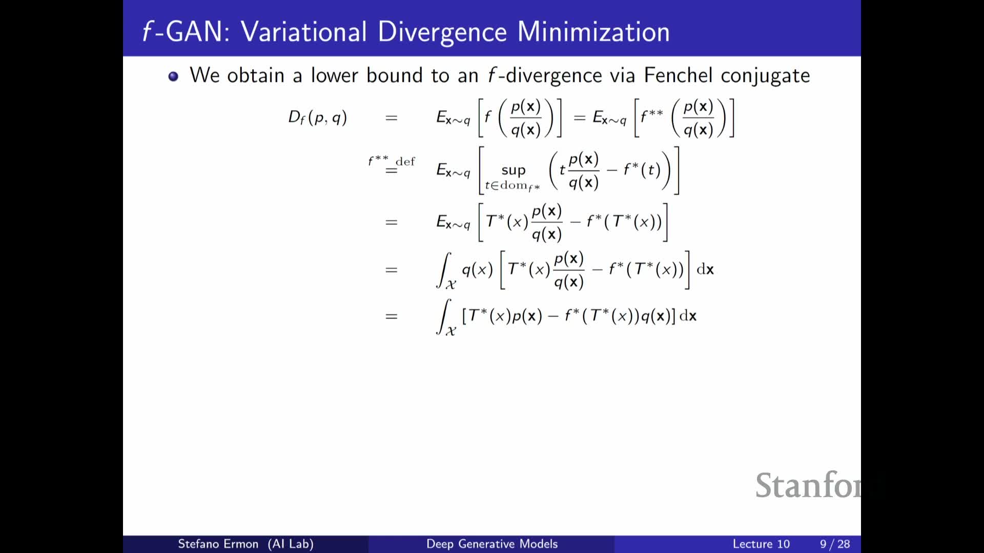
For each x the supremum over t can be represented by a function T(x) that maps x to the optimal t-value.
- Restricting T to a parametric family (e.g., neural networks parameterized by φ) converts the pointwise supremum into a tractable inner maximization over φ.
- Evaluating the resulting expression yields the objective: E_{x~P}[ T(x) ] − E_{x~Q}[ f*( T(x) ) ], which can be approximated with Monte Carlo samples from P (data) and Q (model).
Training becomes a minimax procedure: maximize this lower bound over φ (the discriminator/witness) and minimize over θ (the generator).
Numbered training flow:
- Sample real data x ~ P and latent z ~ p(z), compute generated samples G_θ(z).
- Update φ by gradient ascent to increase E_P[T_φ(x)] − E_Q[f*(T_φ(x))].
- Update θ by gradient descent to reduce the bound (i.e., make generated samples harder to distinguish).
The bound is tight if the discriminator family is sufficiently expressive and the inner maximization is solved well.
F-GAN formulates a practical minimax objective that approximately minimizes a chosen f-divergence by alternating discriminator and generator updates
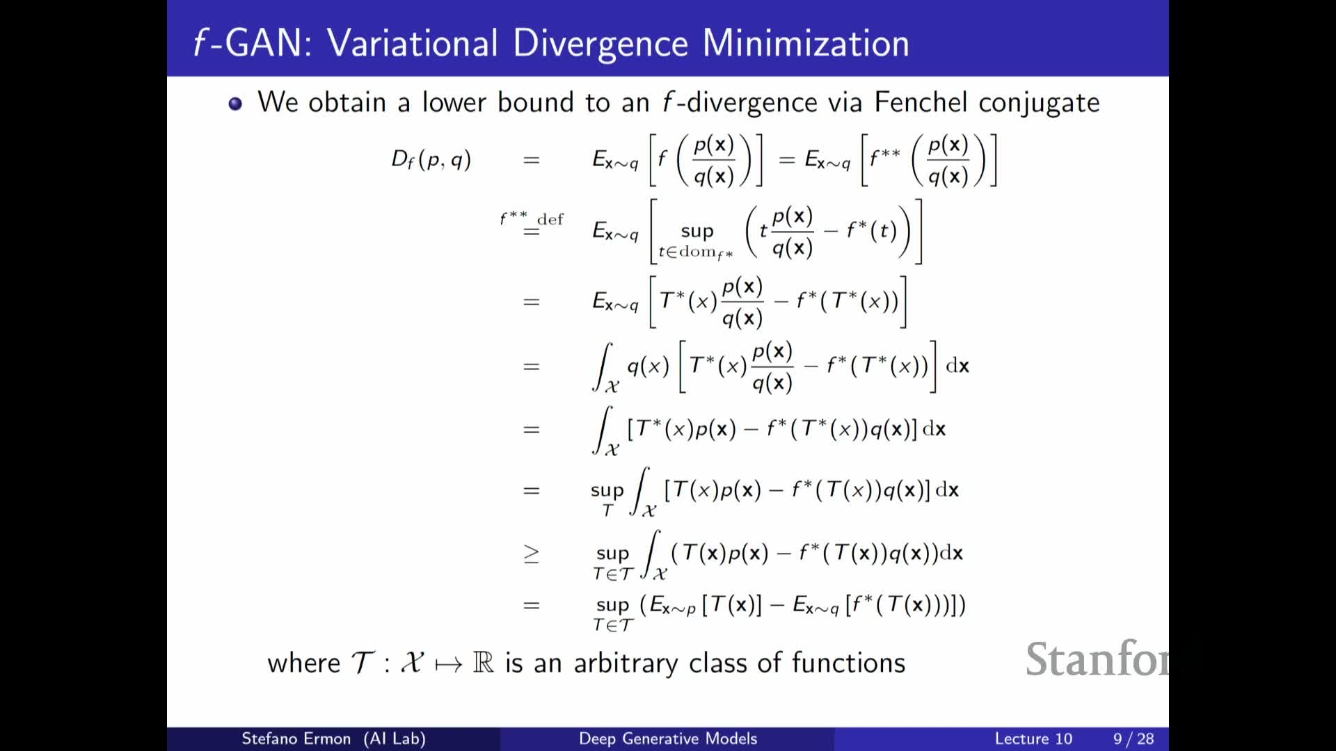
The f-GAN training objective sets up the minimax optimization
min_{θ} max_{φ} [ E_{x~P_data}[ T_φ(x) ] − E_{z~p(z)}[ f*( T_φ( G_θ(z) ) ) ] ],
where G_θ defines the implicit model Q_θ via sampling from a prior p(z), and T_φ is a neural-network witness that approximates the conjugate supremum.
- Selecting different f functions yields different divergences: the f for u log u recovers KL-like behavior; the f that gives Jensen–Shannon recovers the original GAN objective up to constants.
- In practice this provides a likelihood-free estimator of an f-divergence up to the approximation power of the discriminator.
Caveats: minimizing an approximate lower bound can succeed empirically but may inherit bias from limited discriminator capacity and finite-sample optimization errors.
The Wasserstein (Earth Mover) distance measures distribution mismatch via optimal transport and remains meaningful when supports are disjoint
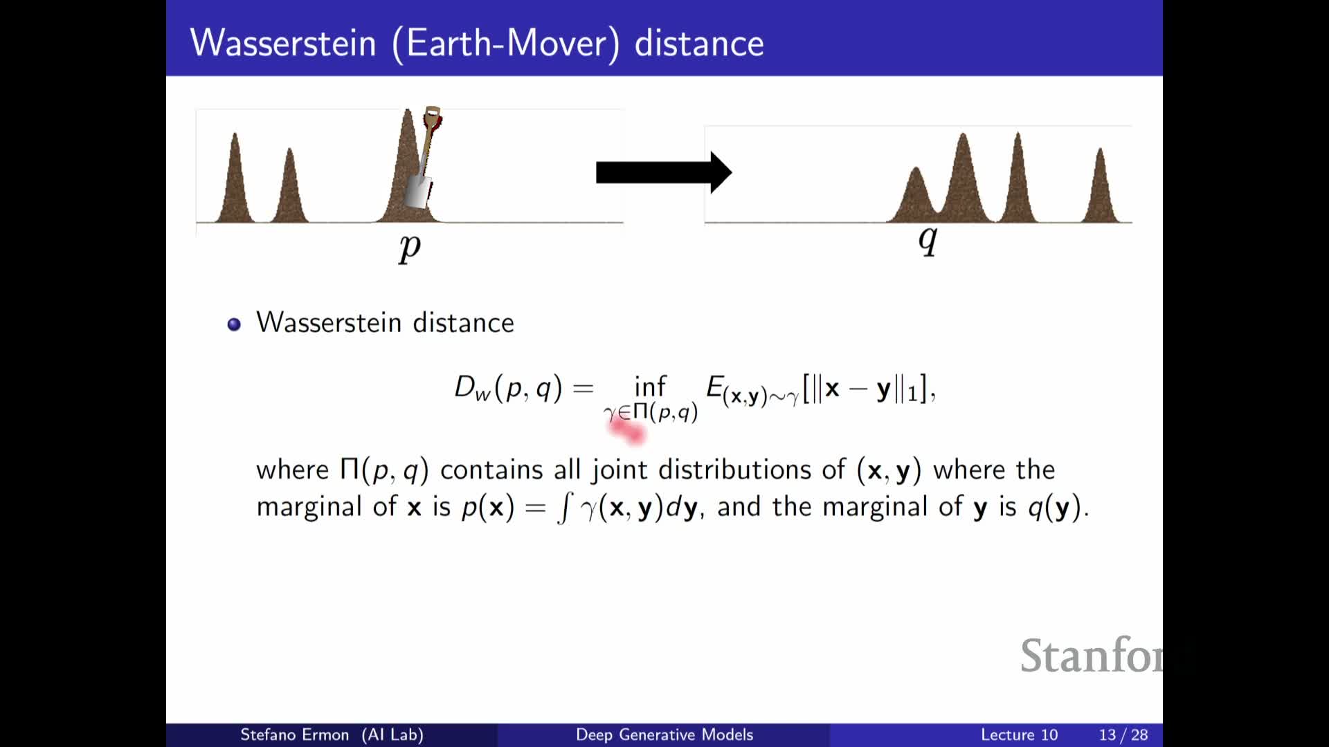
The Wasserstein-1 distance (earth mover distance) quantifies discrepancy by the minimal expected transport cost required to move probability mass from distribution P to distribution Q:
W(P,Q) = inf_{γ ∈ Γ(P,Q)} E_{(x,y)~γ}[ c(x,y) ], where Γ(P,Q) is the set of couplings with marginals P and Q and c(x,y) is a ground cost (commonly L1 or L2 distance).
- The primal (transport) formulation interprets probability mass as piles of earth and seeks an optimal transport plan γ that moves mass with minimal total cost.
- It is well-defined even when P and Q have disjoint supports, avoiding pathological constant or infinite values that can arise with some f-divergences.
- The transport formulation is a linear program over couplings and provides a metric with smooth sensitivity to small changes in support location, yielding richer gradient information for generator updates when supports are initially disjoint.
The Kantorovich–Rubinstein dual expresses Wasserstein-1 as a supremum over 1-Lipschitz witness functions, enabling a GAN-style critic when Lipschitzness is enforced
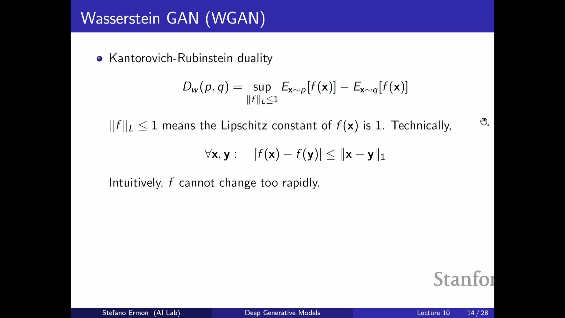
The dual form of the Wasserstein-1 distance is:
W(P,Q) = sup_{f: Lip(f) ≤ 1} [ E_{x~P}[ f(x) ] − E_{x~Q}[ f(x) ] ], i.e., the supremum over all scalar functions f with Lipschitz constant ≤ 1 yields the optimal transport cost.
- This converts the intractable coupling optimization into a variational optimization over a function space and suggests training a parametrized critic network f_φ to approximate the supremum.
- Enforcing the Lip≤1 constraint is critical; practical approximations include weight clipping or gradient penalties on the critic.
The resulting minimax training is: min_{θ} max_{φ, Lip≤1} E_{x~P}[ f_φ(x) ] − E_{z~p(z)}[ f_φ( G_θ(z) ) ], which serves as a practical surrogate for the Wasserstein distance and often yields smoother gradients for the generator.
Wasserstein-GAN objectives mitigate vanishing gradients and training instability common with JS/KL-based GANs but require careful enforcement of the Lipschitz constraint
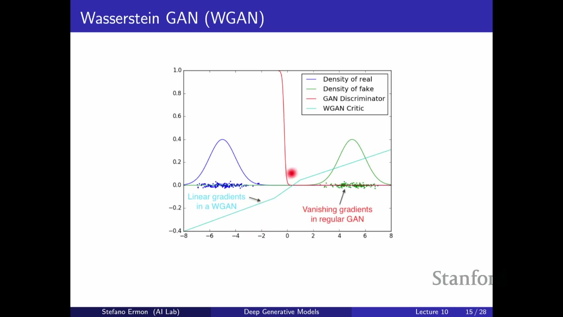
Wasserstein-based critics produce loss landscapes that vary smoothly as the generator distribution moves, addressing regimes where JS or KL are flat or infinite due to disjoint supports and where discriminator outputs lead to vanishing or unstable generator gradients.
- Empirically, this smoother signal often stabilizes training and helps the generator learn meaningful updates even when initial samples are far from data.
- The benefit depends on adequately constraining the critic’s Lipschitz constant; practical strategies include:
-
Weight clipping (simple but can limit expressivity).
-
Gradient-norm penalties (e.g., penalize ∇_x f_φ(x) − 1) which more directly encourage 1-Lipschitz behavior.
-
Weight clipping (simple but can limit expressivity).
These approximations introduce their own limitations and do not guarantee exact equivalence to the true Wasserstein distance, yet they commonly improve stability in large-scale neural GAN training.
Bi-directional GAN variants introduce an encoder to infer latent variables by training a discriminator on joint (data,latent) pairs
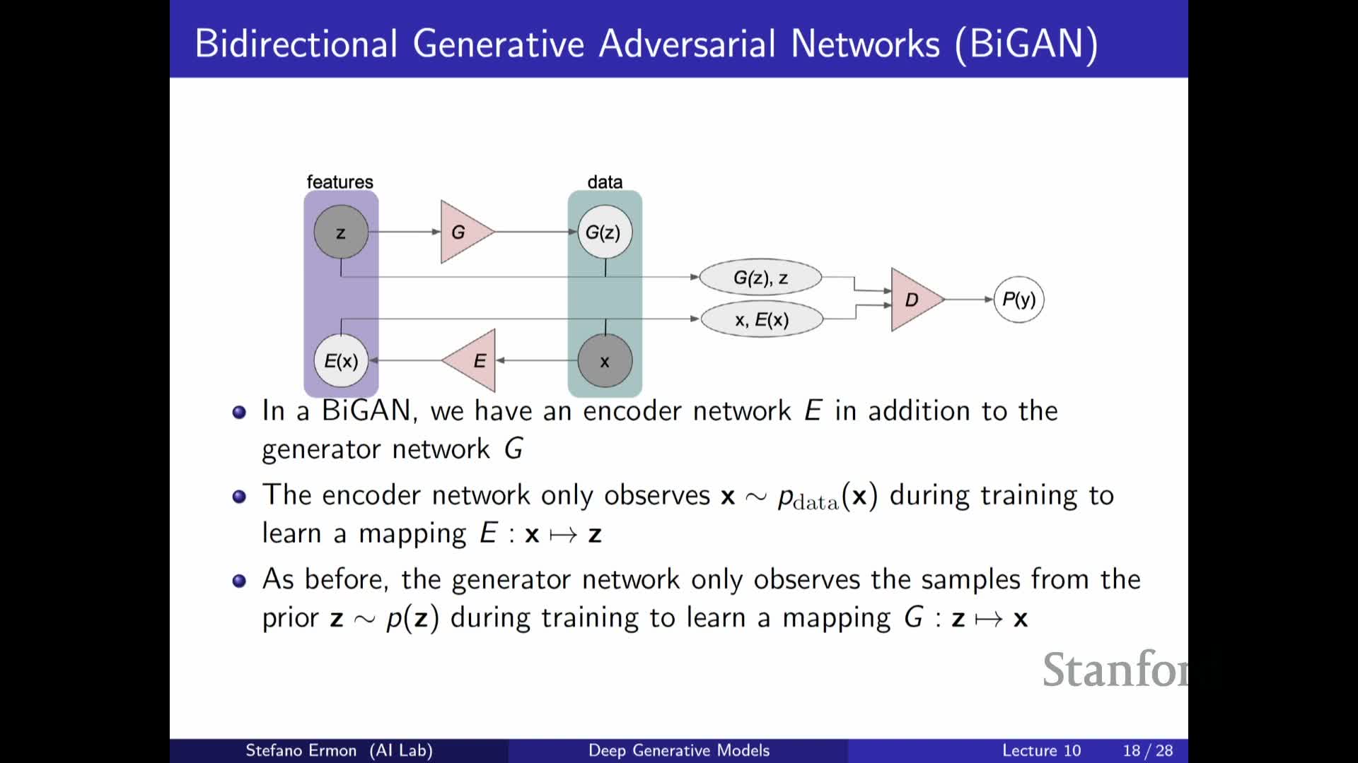
Latent inference in GANs augments the generator G(z) → x with an encoder E(x) → z and trains a discriminator that operates on paired inputs (x, z) to distinguish joint samples from two joint distributions.
- Model joint samples: ( G(z), z ) with z ~ prior p(z).
- Encoder joint samples: ( x, E(x) ) with x ~ data.
The discriminator learns to differentiate model-generated pairs from encoder-produced pairs, while the encoder and generator are trained adversarially to make the two joint distributions indistinguishable.
- When successful, the encoder approximates the inverse of the generator and provides latent embeddings for real data.
- This bi-directional adversarial training (e.g., BiGAN, ALI) yields a deterministic encoder mapping observed x to latent z without requiring tractable likelihoods or KL penalties.
- At inference time the encoder is used to obtain features for downstream tasks; the training objective enforces consistency between prior samples and encoder outputs via adversarial two-sample testing rather than explicit variational bounds.
Enjoy Reading This Article?
Here are some more articles you might like to read next: