Stanford CS236- Deep Generative Models I 2023 I Lecture 11 - Energy Based Models
- Lecture overview and generative model design space
- Likelihood-based models impose structural constraints to ensure valid densities
- Motivation for energy based models as a flexible probabilistic parametrization
- Probabilistic models must satisfy non-negativity and normalization constraints
- Why normalization is hard and how to form normalized densities from unnormalized functions
- Partition function concept, normalization by division, and consequences
- Classical examples and the exponential family as normalized quotients
- Relations between normalized-model constructions and compositional architectures
- Formal definition of an energy based model and choice of exponential parametrization
- Expressivity vs. computational costs: sampling and likelihood evaluation challenges
- Curse of dimensionality and implications for partition function estimation
- Tasks that do not require explicit partition function evaluation
- Derivative-based properties and model composition via product or mixture ensembles
- Product-of-experts behavior and sampling considerations
- Restricted Boltzmann Machine (RBM) as a discrete latent-variable energy model
- Partition function in RBMs and why exact likelihood training is infeasible
- Gradient of the log-likelihood and the contrastive-divergence Monte Carlo approximation
- Sampling from EBMs using local proposals and Markov chain Monte Carlo
Lecture overview and generative model design space
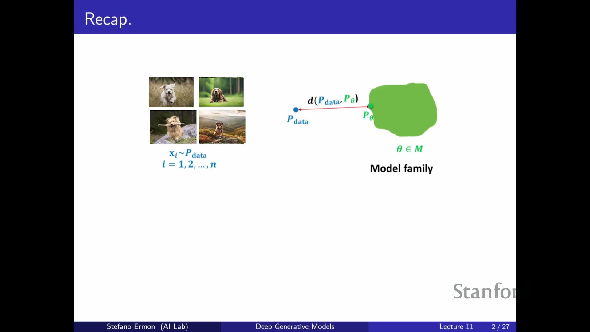
The lecture introduces energy-based models (EBMs) as a family of generative models and situates them within the general design space for generative modeling: choose a model family and a loss function given IID data samples.
Principled objectives like maximum likelihood and Kullback–Leibler (KL) divergence are appropriate when models provide tractable likelihoods. This motivates architectures that allow exact or approximate density evaluation, such as autoregressive models and normalizing flows.
The central tradeoff is framed clearly:
- Models that permit likelihood evaluation impose architectural constraints.
-
Likelihood-free or implicitly defined samplers (for example, GANs) relax those constraints but require alternative training objectives and often unstable minimax optimization.
This tension motivates exploring EBMs, which aim to combine high flexibility in parameterizing distributions with likelihood-informed or likelihood-based training strategies.
Likelihood-based models impose structural constraints to ensure valid densities
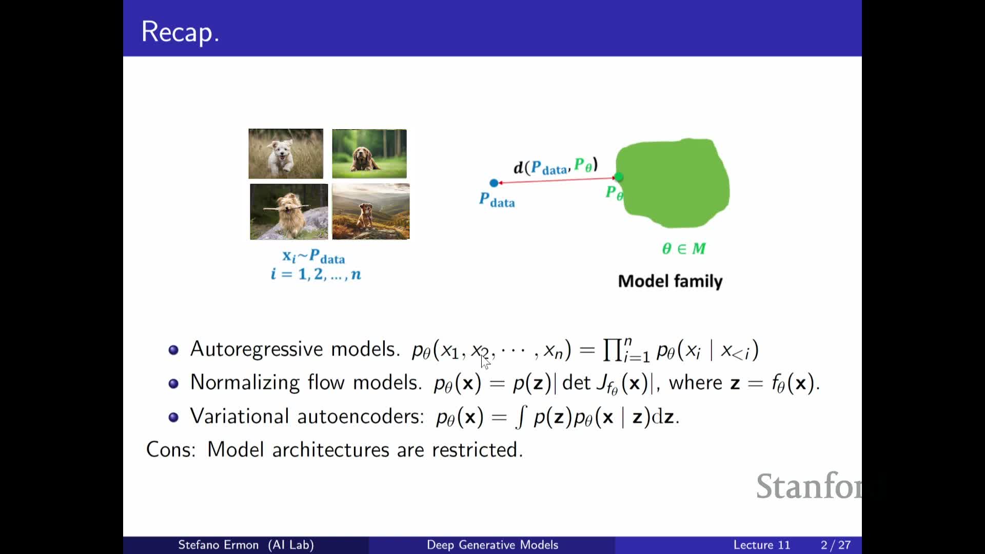
Models that permit direct likelihood evaluation must satisfy two constraints: non-negativity and normalization. Enforcing these constraints forces particular architectural designs:
-
Autoregressive constructions: use the chain rule to produce normalized conditionals.
-
Invertible networks / flows: produce a tractable change-of-variables Jacobian for exact density evaluation.
-
Latent-variable / variational approaches: use analytic or approximated marginalization.
These constraints limit admissible neural architectures because arbitrary networks do not automatically yield valid probability densities.
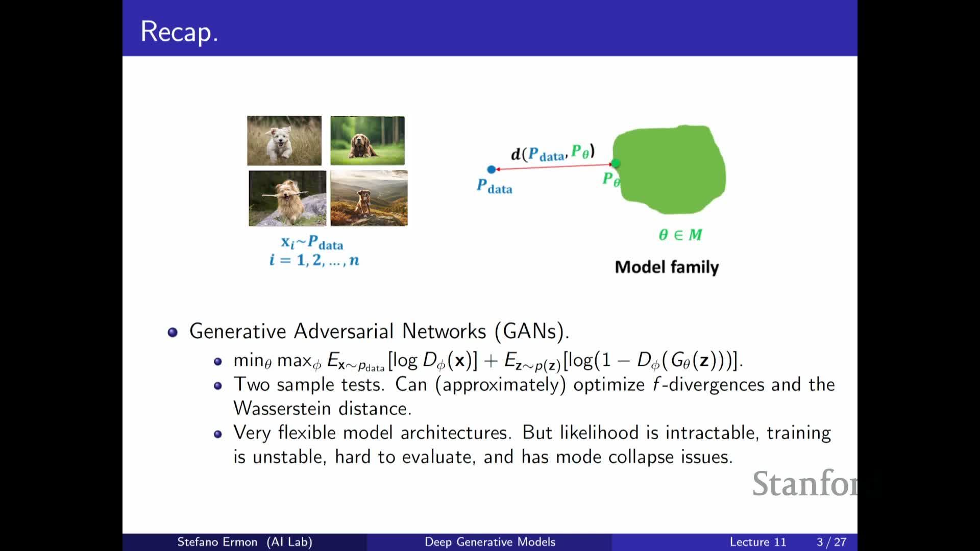
When likelihood evaluation is infeasible, alternative approaches like GANs define the model implicitly via a sampler and use two-sample tests or discriminator-based objectives to train. However, these minimax objectives introduce:
- training instability,
- difficulty detecting convergence,
- challenges for principled evaluation.
The lecture emphasizes these practical costs and motivates methods that recover architectural flexibility without abandoning principled training entirely.
Motivation for energy based models as a flexible probabilistic parametrization
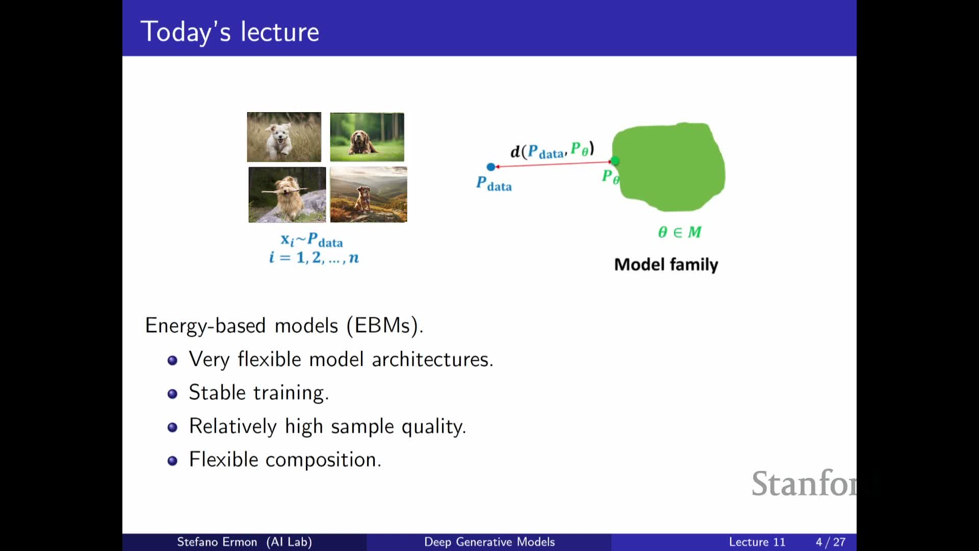
Energy-based models (EBMs) lift many architectural restrictions by defining distributions implicitly via an unnormalized energy or score function.
- EBMs allow essentially arbitrary neural network architectures to output a scalar energy for any input.
-
Normalization is enforced by dividing the unnormalized density by a partition function, enabling very expressive model families.
The lecturer highlights connections to maximum likelihood and related losses, suggesting EBMs can yield more stable training than adversarial methods while retaining links to likelihood-informed objectives.
EBMs are also closely related to diffusion models, which have achieved state-of-the-art sampling in continuous domains, and to compositional modeling: EBMs can be composed or combined with other model families to capture intersecting concepts.
Probabilistic models must satisfy non-negativity and normalization constraints
A valid probability mass or density function must be non-negative everywhere and integrate (or sum) to one; these two constraints are conceptually distinct in enforcement difficulty.
-
Non-negativity is easy to enforce for arbitrary neural networks by applying elementwise transforms such as squaring, exponentiation, absolute value, or similar final-layer operations that guarantee non-negative outputs.
-
Normalization is far more restrictive: it requires the integral or sum over the entire domain to equal a constant independent of parameters. This typically forces special architectures (autoregressive factorization, invertible transforms) or analytic functional choices.
The lecture uses an analogy of dividing a cake among outcomes to emphasize that enforcing a fixed total mass is the primary challenge motivating alternative formulations like EBMs.
Why normalization is hard and how to form normalized densities from unnormalized functions
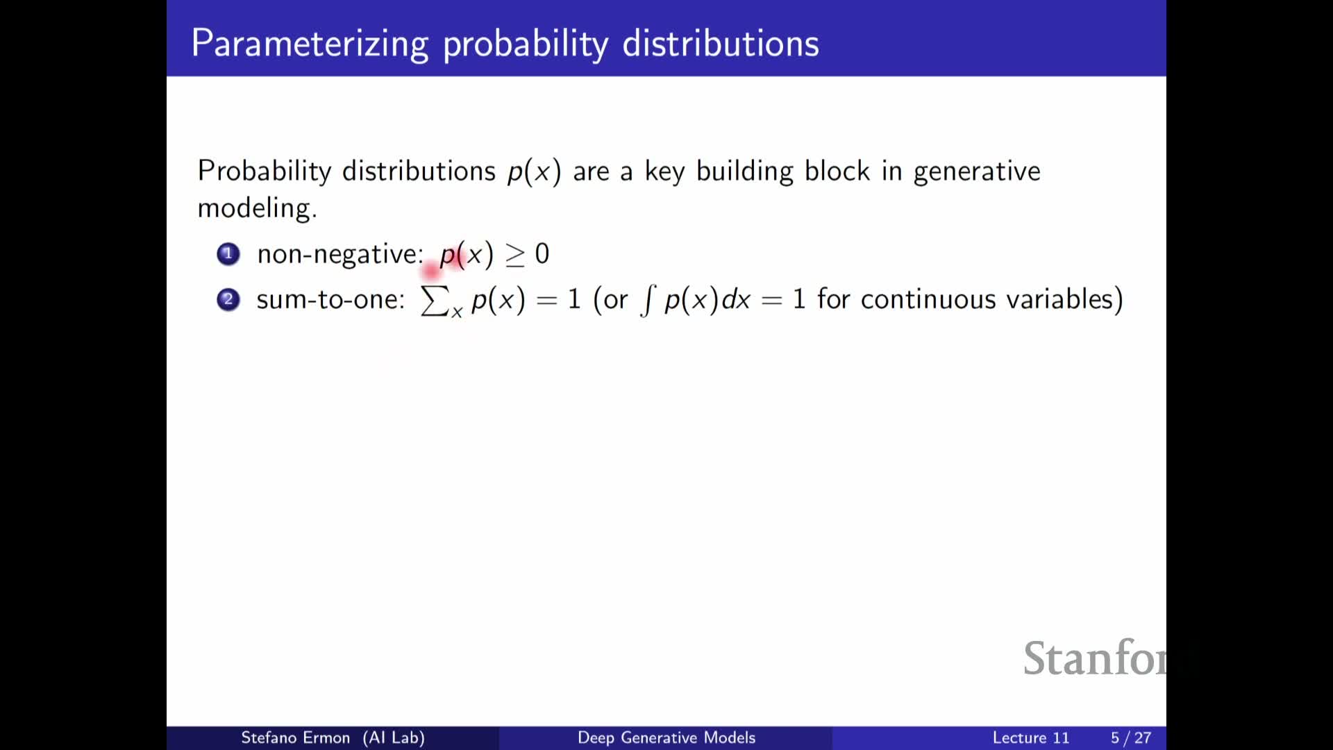
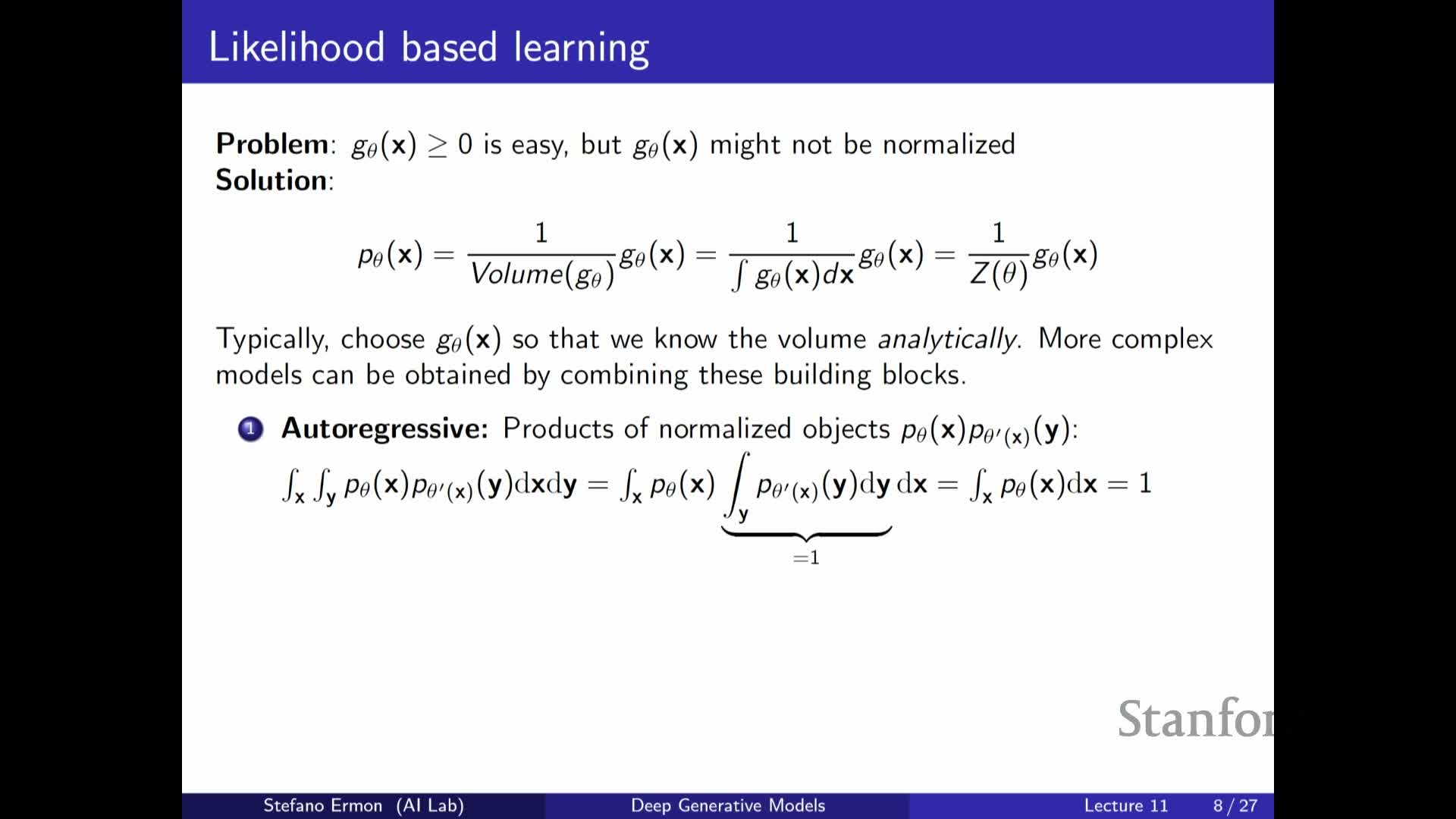
Given an arbitrary parameterized non-negative function G_theta(x) produced by a neural network, the total integral (or sum) over x is generally a parameter-dependent scalar and will not equal one by default.
Energy-based modeling embraces this by defining a normalized density:
- p_theta(x) = G_theta(x) / Z_theta,
where Z_theta is the partition function (the integral or sum of G_theta over the domain). This division produces a valid probability distribution for any non-negative G_theta.
However, computing Z_theta analytically is feasible only for restricted functional forms. EBMs therefore acknowledge that Z_theta is typically intractable and must be handled explicitly—either approximated or avoided by algorithmic design. This reparameterization opens the door to highly flexible G_theta choices while making clear the computational bottleneck: the partition function.
Partition function concept, normalization by division, and consequences
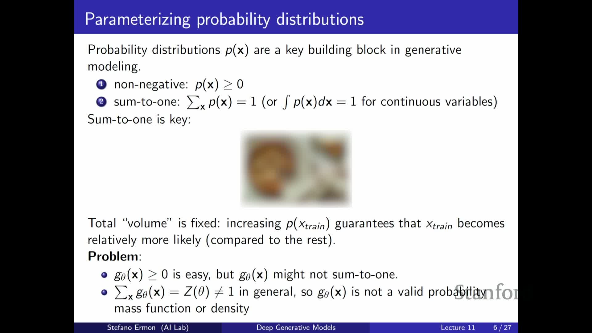
Dividing a non-negative unnormalized density by its partition function yields a mathematically valid normalized probability model, which is the defining construction of EBMs.
-
Z_theta is the integral (continuous case) or sum (discrete case) of the unnormalized function and depends on parameters, so it must be considered during evaluation and learning.
- In simple families (e.g., Gaussian, exponential) this integral can be computed in closed form, yielding classical normalized distributions.
For general neural-network-parameterized unnormalized functions, Z_theta is intractable due to the curse of dimensionality and exponential growth in domain size. Therefore, EBMs trade expressivity for the need to either approximate Z_theta or develop training and sampling methods that avoid requiring its exact value.
Classical examples and the exponential family as normalized quotients
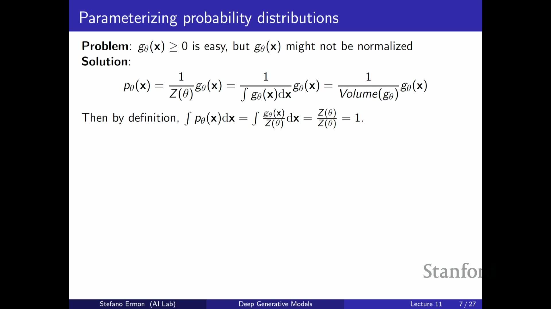
Many familiar distributions fit the unnormalized-plus-division pattern:
-
Gaussian: exp(−(x−μ)^2/(2σ^2)) divided by sqrt(2πσ^2).
-
Exponential: exp(−λx) divided by 1/λ.
More generally, distributions in the exponential family take the form p(x) ∝ exp(θ·T(x)) with a log-partition function that normalizes the density; these families are analytically tractable under specific sufficient-statistic choices and capture a wide class of common distributions.
The lecture explains that EBMs generalize this paradigm by allowing complex neural-network-based energies in the exponent, removing the requirement that normalization be analytically solvable. This extension increases modeling flexibility but transfers the computational burden to approximating or otherwise handling the partition function during learning and inference.
Relations between normalized-model constructions and compositional architectures
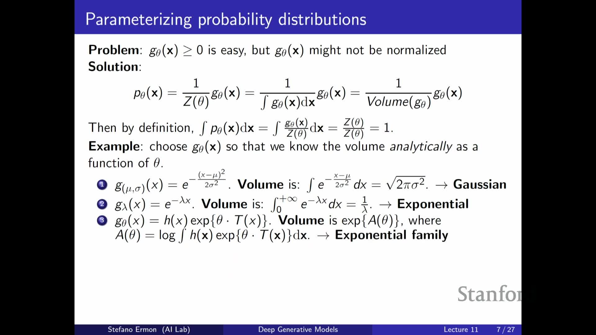
Autoregressive models, latent-variable models, flows, and mixtures can be interpreted as structured ways to build complex normalized densities from simpler normalized components:
-
Autoregressive: the joint is a product of normalized conditionals, so the full joint is normalized by design.
-
Latent-variable: marginalizing over simple normalized conditionals yields normalized marginals.
-
Flows: use invertible transforms with tractable Jacobians to convert between densities.
-
Mixtures: convex combinations of normalized components remain normalized.
These constructive approaches guarantee normalization for all parameter settings, but they impose design constraints and may limit flexibility compared to arbitrary unnormalized energies. EBMs are contrasted as freeing architecture choices at the cost of making the normalization constant parameter-dependent and generally intractable.
Formal definition of an energy based model and choice of exponential parametrization
An energy-based model parameterizes a probability density as:
-
p_theta(x) = exp(f_theta(x)) / Z_theta, where f_theta(x) is an arbitrary scalar-valued function (often a neural network) and Z_theta is the partition function.
- The exponential map guarantees non-negativity and conveniently models large dynamic ranges in relative probabilities: small changes in f_theta can yield large multiplicative changes in p_theta(x).
- This form generalizes softmax-style normalization for finite discrete outputs and recovers classical exponential-family forms when f_theta is simple.
The primary practical costs are that evaluating normalized probabilities and drawing samples are difficult because Z_theta is generally intractable for high-dimensional x.
Expressivity vs. computational costs: sampling and likelihood evaluation challenges
EBMs provide maximal flexibility in choosing f_theta, enabling arbitrary neural architectures to model data. But this flexibility incurs computational costs:
- Evaluating normalized likelihoods requires computing Z_theta.
- Sampling from p_theta(x) is typically expensive or intractable by straightforward methods because Z_theta couples probabilities across the entire domain.
Numerical integration or brute-force summation scales exponentially with dimensionality and is infeasible for images, audio, and other high-dimensional modalities. The lecturer notes that diffusion models effectively exploit energy-based parametrizations and approximations to achieve strong sampling performance, illustrating that the flexibility payoff can be realized with careful algorithm design.
Overall, EBMs trade architectural freedom for the need to employ sophisticated approximations for inference, sampling, and training.
Curse of dimensionality and implications for partition function estimation
The central computational barrier for EBMs is the curse of dimensionality: the number of domain configurations grows exponentially with the number of variables, so exact computation of Z_theta or naive numerical approximations are infeasible.
- This affects discrete domains (combinatorial explosion of assignments) and continuous domains (volume discretization required to approximate integrals).
- Likelihood-based training and exact sampling become prohibitive for high-dimensional data.
Consequently, practical EBM algorithms focus on methods that either bypass the need to compute Z_theta exactly (e.g., contrastive objectives, score-based formulations) or approximate the partition function or its gradients with Monte Carlo and MCMC techniques. The lecture frames subsequent material as addressing how to learn and sample from EBMs despite this fundamental complexity.
Tasks that do not require explicit partition function evaluation
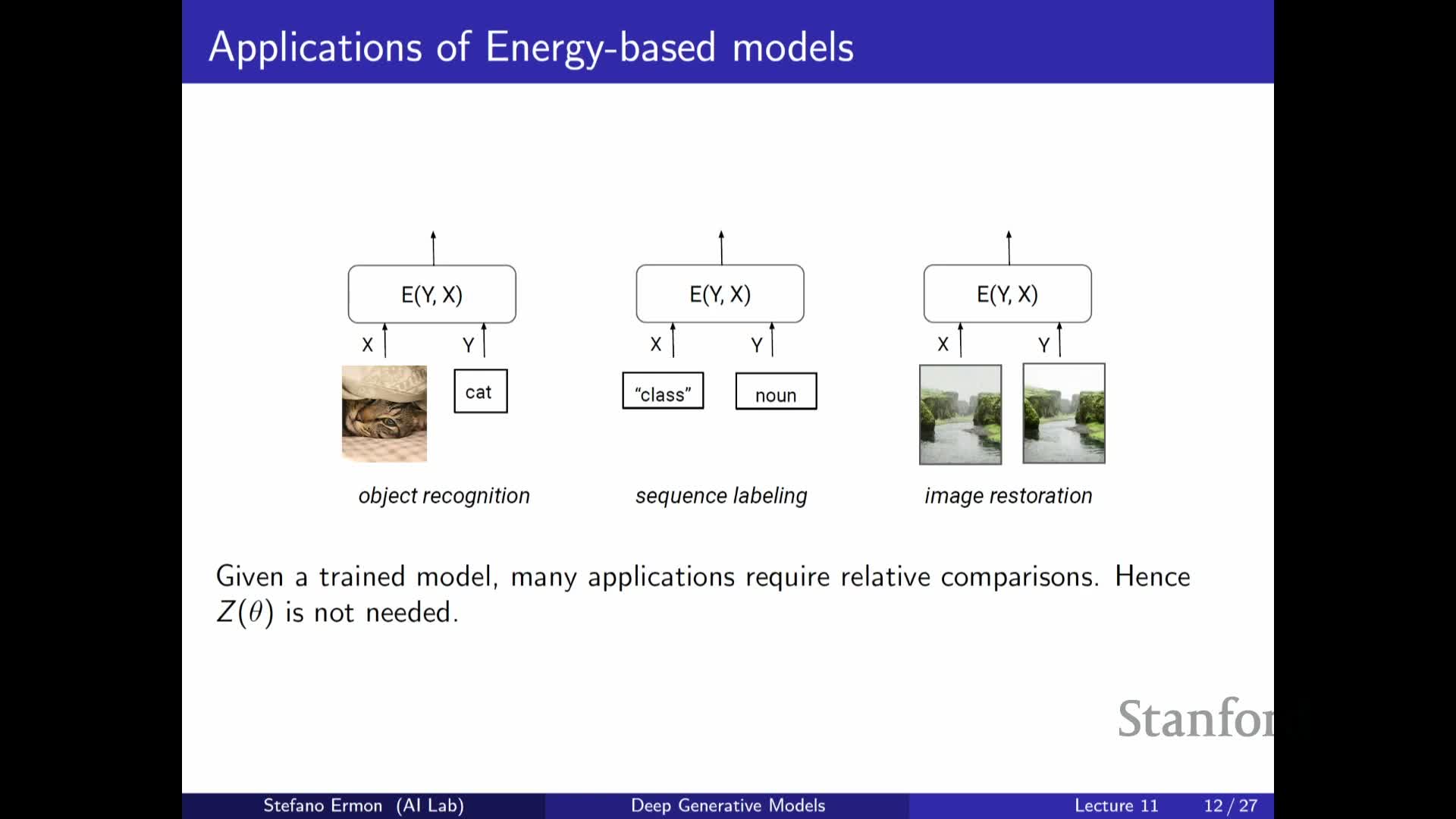
Many practical tasks require only relative comparisons between model scores rather than absolute normalized probabilities, so the partition function cancels out in ratios and can be ignored for those tasks.
Examples include:
-
Ranking
-
Anomaly detection
-
Conditional MAP inference (finding argmax_y p(y x))
- Many discriminative tasks where only relative orderings of likelihoods matter
| The lecture illustrates denoising as a conditional inference problem where the posterior mode argmax_y p(y | x) can be found without knowing Z_theta because normalization over y given x is constant across candidate y values. This property makes EBMs useful for a range of applications despite the intractability of Z_theta and motivates sampling and optimization techniques that exploit score comparisons. |
Derivative-based properties and model composition via product or mixture ensembles
The gradient of the log-probability with respect to parameters often eliminates dependence on the partition function in useful ways, enabling learning algorithms that do not require Z_theta explicitly because derivatives of log p_theta(x) remove additive constants.
Energy-based representations also enable flexible ensembling operations:
-
Product-of-experts: multiplying normalized model densities yields an unnormalized product whose log-energy is the sum of individual log-densities. This behaves like an AND operator—any expert assigning near-zero probability drives the product low—enabling composition that captures intersections of concepts. However, the product requires renormalization with a global partition function, reintroducing computational costs for sampling and likelihood evaluation.
-
Mixtures: convex combinations behave like a soft OR and remain normalized by construction, but they do not impose intersection constraints and are easier to work with when component partition functions are known.
Product-of-experts behavior and sampling considerations
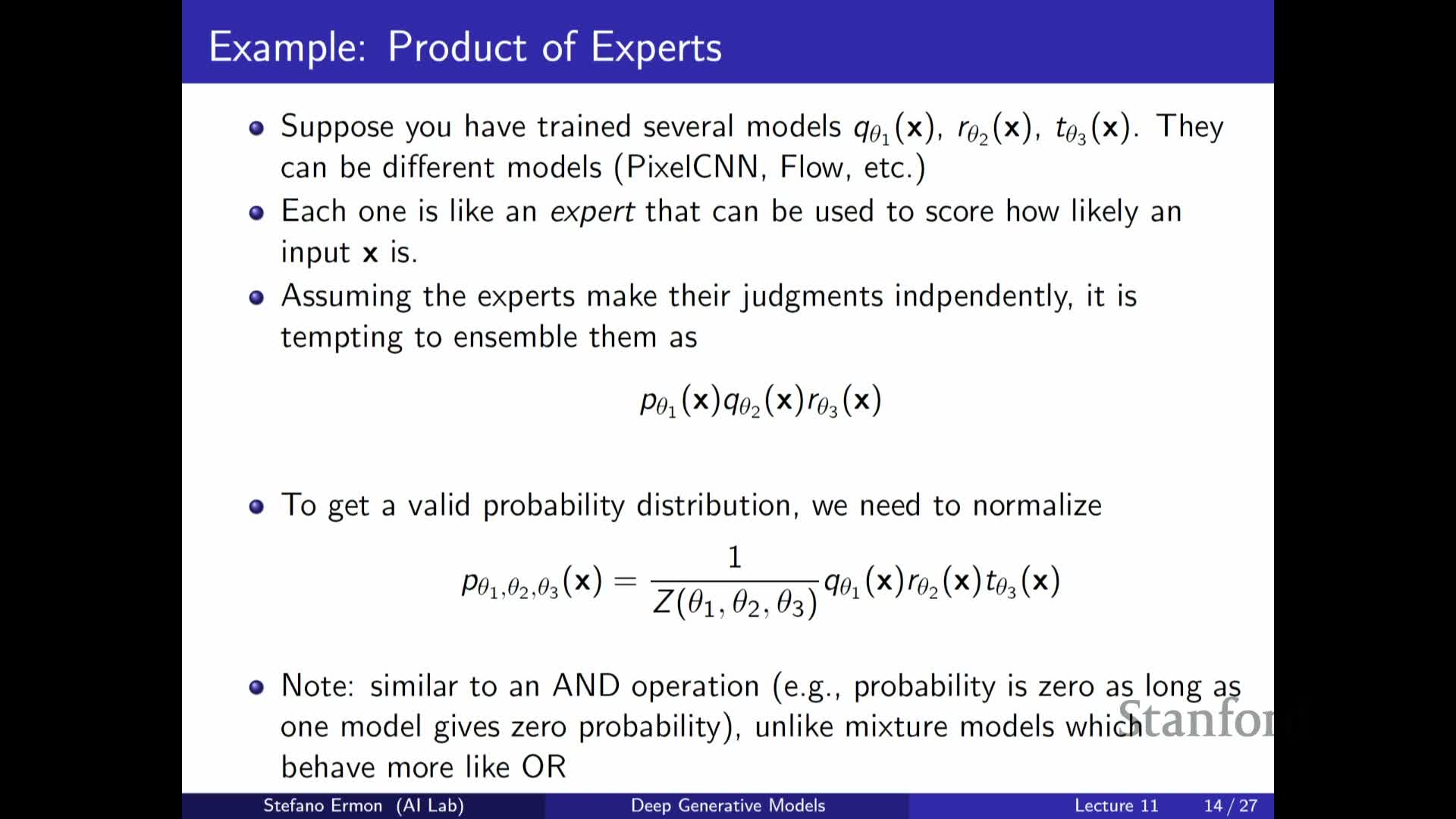
The product-of-experts approach multiplies individual densities to produce a combined unnormalized density whose energy is the sum of component energies. Key points:
- The combined model emphasizes intersections of support across experts (semantic compositionality).
- The global partition function for the product must be computed or approximated to normalize the model.
-
Sampling from the product is harder than sampling each component independently because the product couples variables and typically requires specialized MCMC or other approximate samplers.
Although sampling is expensive, it is not impossible: practical implementations use approximate inference strategies to make products of experts useful in applications.
Restricted Boltzmann Machine (RBM) as a discrete latent-variable energy model
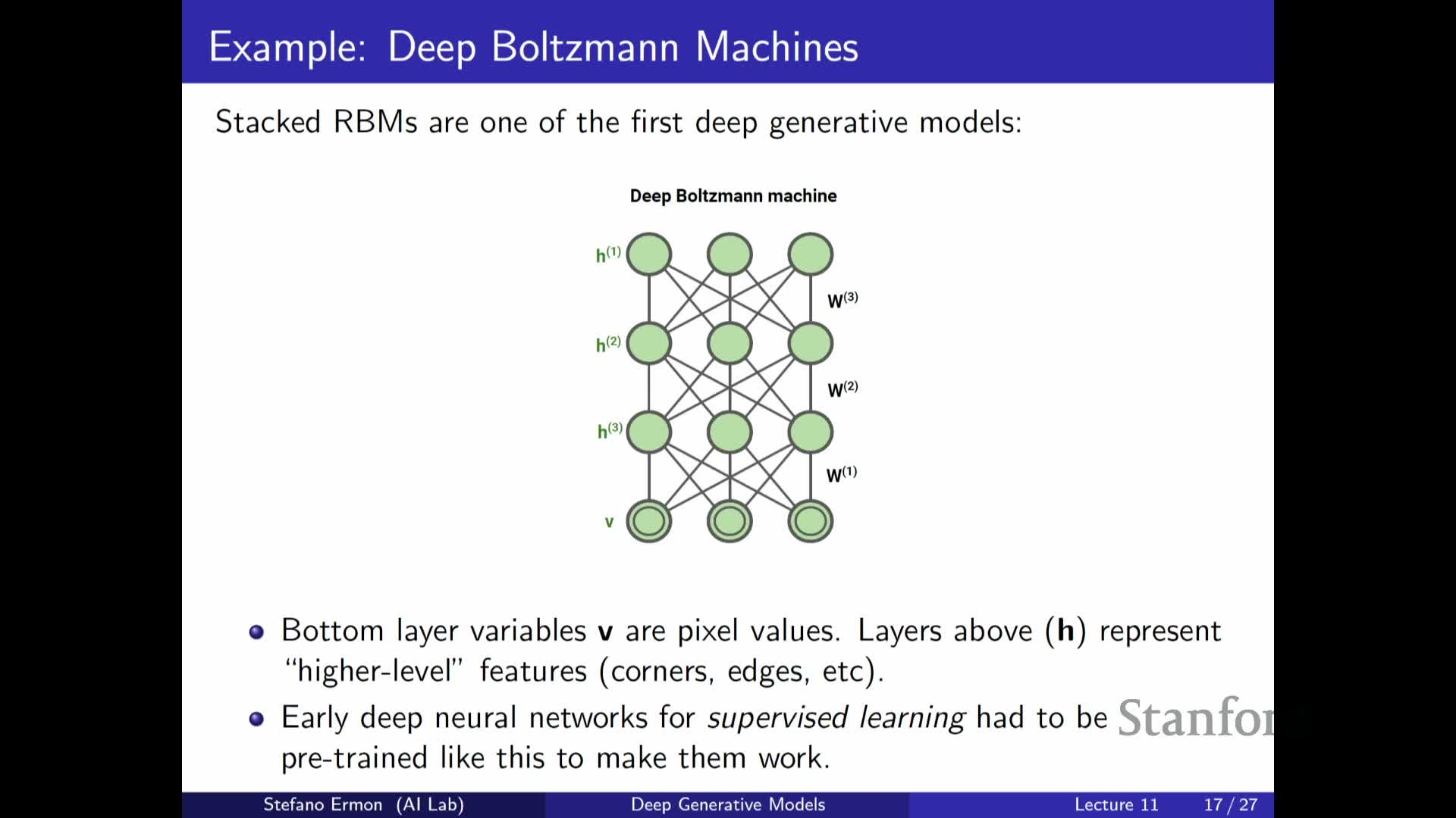
The Restricted Boltzmann Machine (RBM) is a canonical discrete EBM with binary visible variables x and binary hidden variables z, defined by an energy that is a quadratic form comprising visible biases, hidden biases, and pairwise visible–hidden interactions weighted by a matrix W.
- The RBM has no intra-layer interactions (no visible–visible or hidden–hidden terms), which makes conditional sampling between layers tractable and enables efficient Gibbs updates for certain inference steps.
- Historically, RBMs and stacked compositions (Deep Belief Networks) were among the first deep generative models to produce compelling samples and served as unsupervised pretraining for deep supervised networks.
Despite their historical importance, RBMs exemplify the partition function problem, since computing Z requires summing over exponentially many joint assignments of visible and hidden units.
Partition function in RBMs and why exact likelihood training is infeasible
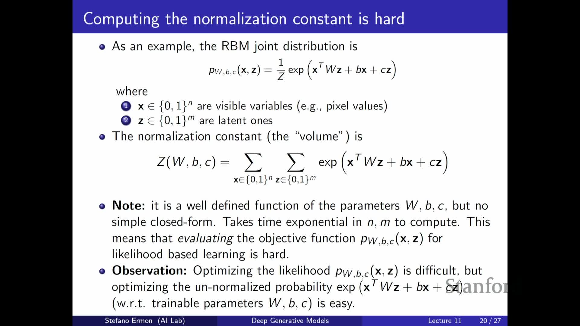
In an RBM the unnormalized probability is straightforward to evaluate for any configuration via the energy computation, but the partition function requires summing exp(−energy) over all 2^n × 2^m combinations of visible and hidden binary variables.
- This exponential summation makes exact computation of normalized probabilities impractical except for very small models, so directly applying maximum likelihood is infeasible at realistic scales.
- Learning therefore relies on approximate methods that either estimate gradients via Monte Carlo sampling or perform specialized approximations that avoid exact evaluation of Z, acknowledging that parameter changes affect both the unnormalized numerator and the partition-function denominator.
The lecture frames contrastive methods as a practical solution to this challenge.
Gradient of the log-likelihood and the contrastive-divergence Monte Carlo approximation
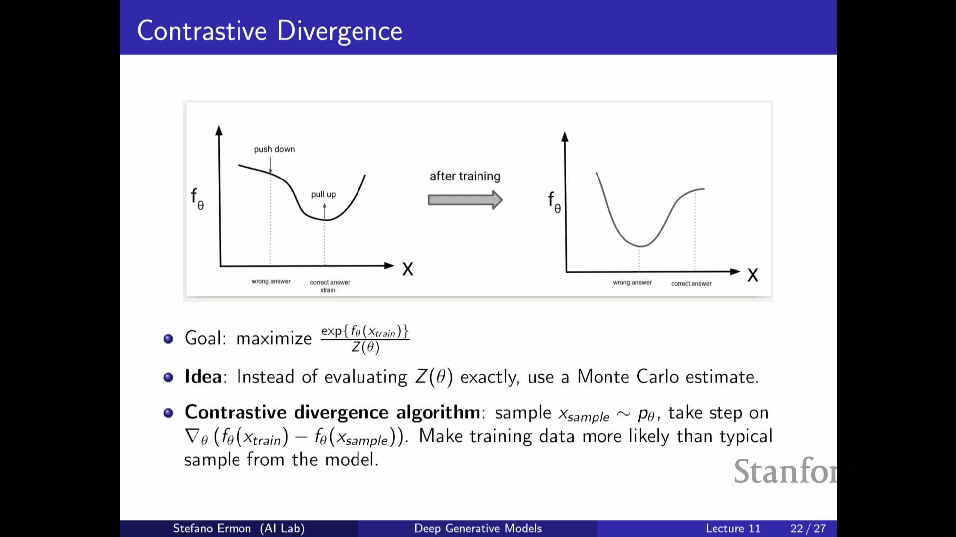
The exact gradient of the log-likelihood for an EBM decomposes into two terms:
- The gradient of the energy evaluated at a data point (the positive term).
- Minus the expected gradient of the energy under the model distribution (the negative term).
The second term is an expectation over the model distribution and therefore depends on Z_theta implicitly; computing it exactly is intractable but it can be approximated with Monte Carlo by drawing samples from the model.
Contrastive Divergence (CD) approximates this expected term with a small number of samples (often one), yielding a low-bias stochastic estimate of the gradient direction that increases the model’s relative probability of observed data compared to typical model samples. This operationalizes the intuitive objective of making training data more likely than typical negative samples drawn from the current model.
Sampling from EBMs using local proposals and Markov chain Monte Carlo
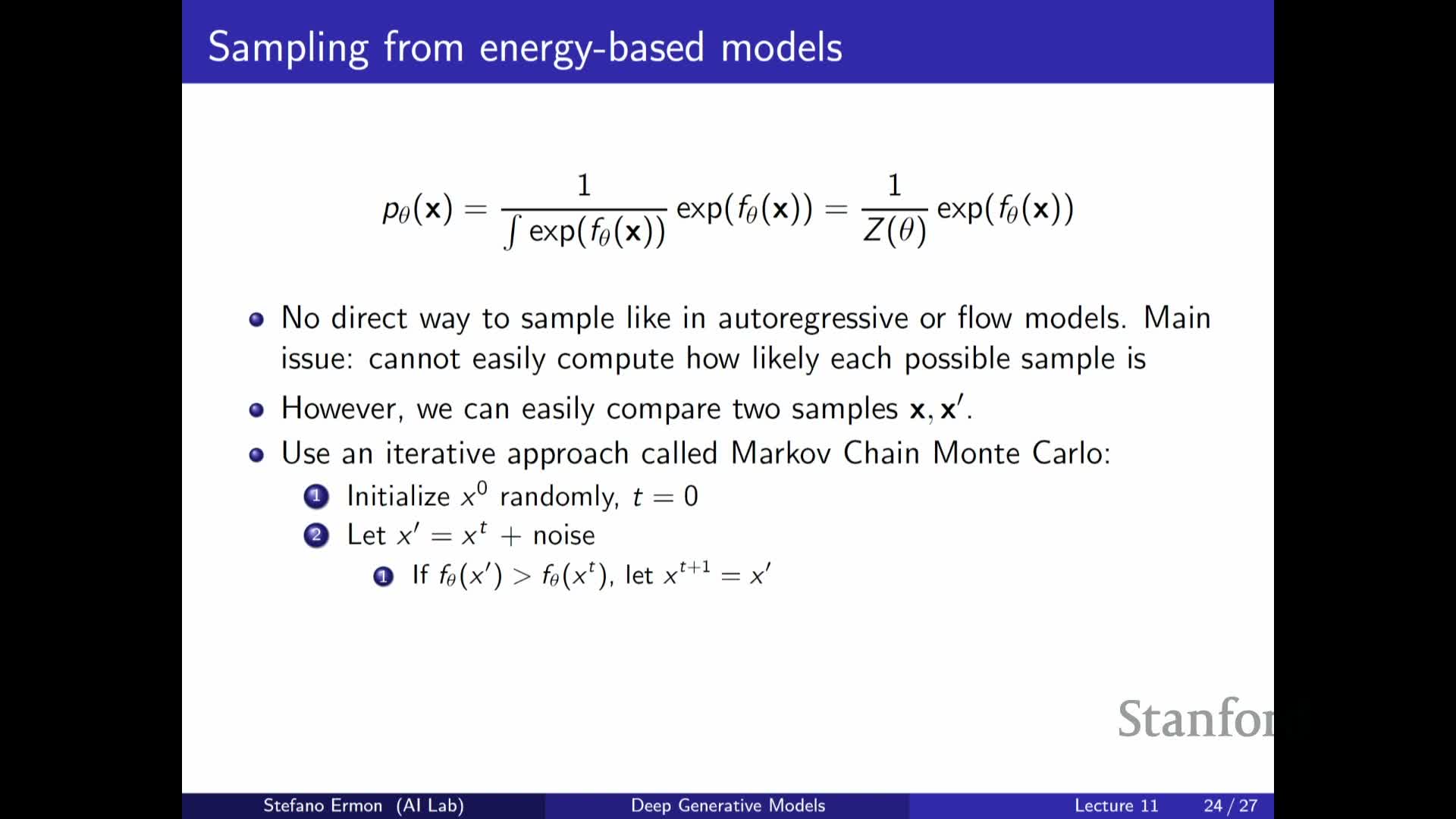
Sampling from high-dimensional EBMs typically uses Markov chain Monte Carlo (MCMC) methods that perform local proposals followed by accept/reject decisions so samples asymptotically follow the target distribution.
A generic MCMC sampling loop looks like this:
- Initialize x (e.g., random or previous state).
- Propose a local perturbation (for example, add noise or make a small move).
- Compare unnormalized probabilities (or energies) of proposed and current states. Uphill (higher-probability) proposals are accepted deterministically; downhill moves are accepted probabilistically according to a Metropolis–Hastings acceptance rule based on the ratio of unnormalized densities.
- Repeat steps 2–3 many times to allow exploration and mixing.
Occasional acceptance of downhill proposals is essential to avoid trapping in local modes and to permit exploration of the state space. Running the chain for sufficiently many iterations yields samples from the true model in the limit.
Practical MCMC for EBMs can be computationally expensive and requires careful proposal design and mixing diagnostics, but it provides a principled mechanism both for sampling and for generating the negative samples used in contrastive learning.
Enjoy Reading This Article?
Here are some more articles you might like to read next: