Stanford CS236- Deep Generative Models I 2023 I Lecture 12 - Energy Based Models
- Energy-based models (EBMs) define probability densities via an unnormalized energy function and a parameter-dependent partition function
- Partition function intractability makes direct likelihood evaluation and maximum likelihood training difficult, but relative probability comparisons are feasible
- Contrastive Divergence estimates likelihood gradients by contrasting training data with samples from the model
- Markov chain Monte Carlo (MCMC) methods enable sampling from EBMs via local proposals and acceptance rules that satisfy detailed balance
- Langevin dynamics and noisy gradient ascent are efficient MCMC proposals for continuous EBMs using score information
- Sampling and contrastive-training costs make naive likelihood-based training of EBMs impractical at scale
- The score function is the gradient of the log-density with respect to the input and does not depend on the partition function
- Score matching and the Fisher divergence compare distributions by their score vector fields and yield a partition-free training objective
- Integration by parts (and its multivariate analogue) converts the Fisher divergence into a computable loss involving model derivatives only
- Practical computation of the score-matching loss requires approximations for second derivatives and scalable estimators such as sliced or denoising score matching
- Noise-contrastive estimation (NCE) trains a classifier to distinguish data from a known noise distribution, yielding density-ratio estimates
- An energy-based discriminator with a learnable partition constant turns NCE into a trainable EBM without inner-loop sampling
- Adapting the noise distribution via parametric flows yields flow-contrastive estimation that jointly trains a tractable generator and an EBM-like discriminator
Energy-based models (EBMs) define probability densities via an unnormalized energy function and a parameter-dependent partition function
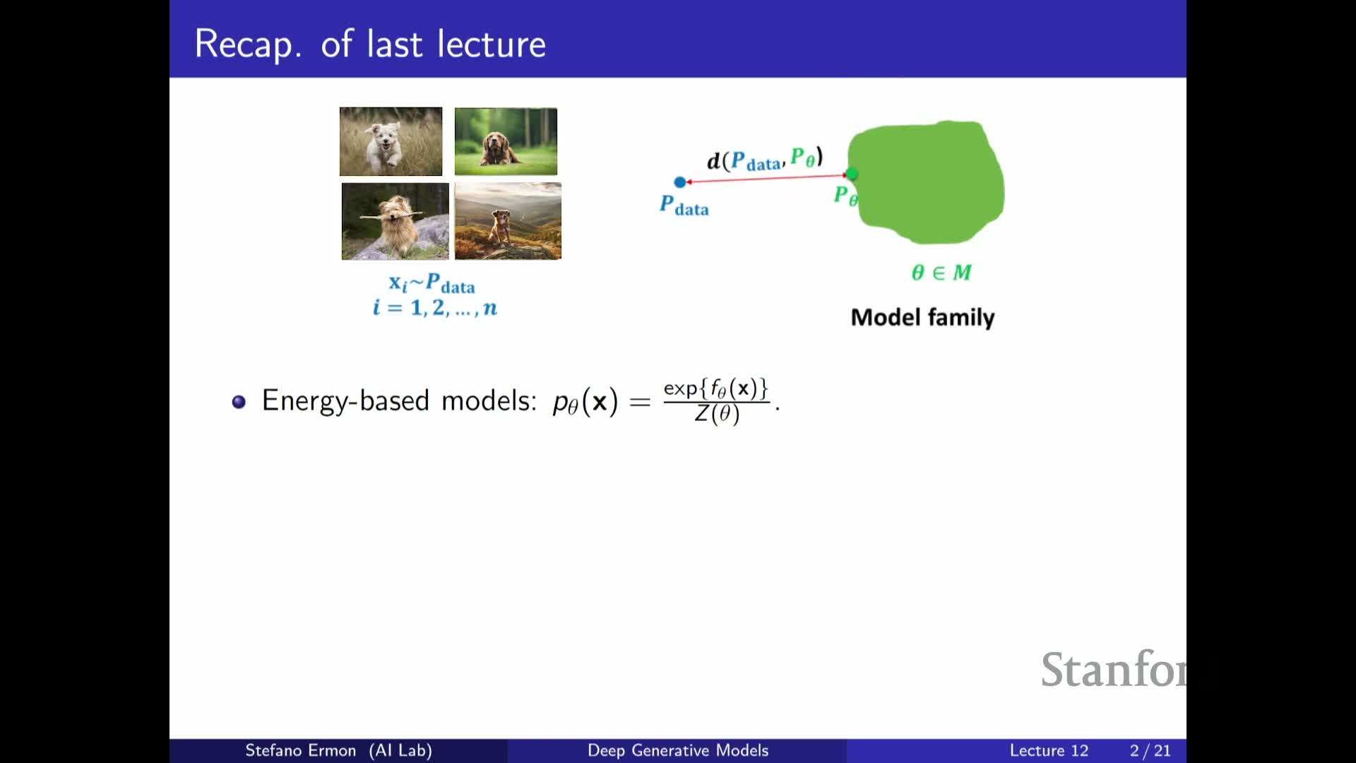
Energy-based models represent probability densities using an energy function f_theta(x) so that the model density is
p_theta(x) = exp(f_theta(x)) / Z(theta), where the partition function Z(theta) normalizes the unnormalized probability.
- The energy function can be any parameterized function (commonly a neural network), which makes EBMs a highly flexible family of distributions.
- The partition function Z(theta) equals the integral or sum of exp(f_theta(x)) over the sample space and depends on the model parameters, so likelihood values are meaningful only relative to Z(theta).
- Because Z(theta) couples all possible x values, evaluating exact normalized likelihoods typically becomes computationally intractable in high-dimensional settings.
Partition function intractability makes direct likelihood evaluation and maximum likelihood training difficult, but relative probability comparisons are feasible
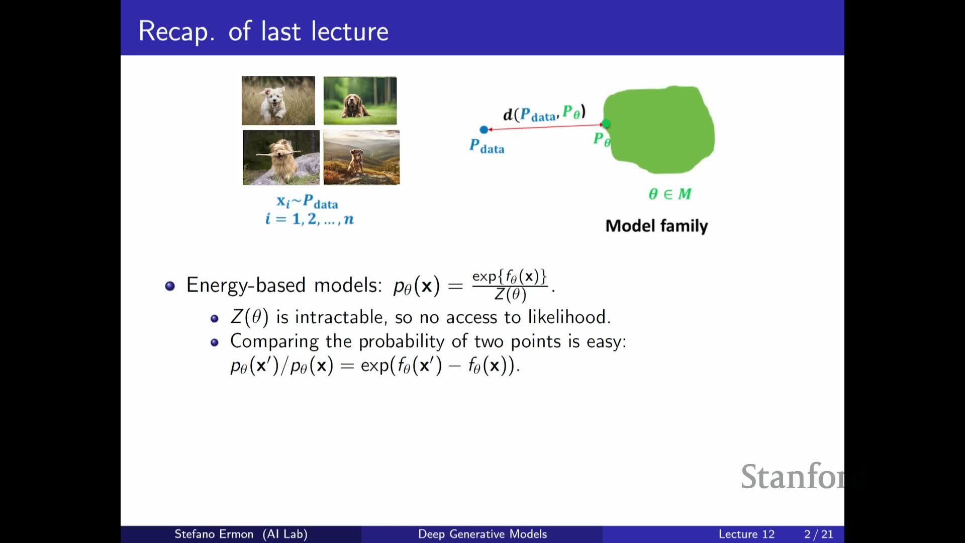
The partition function Z(theta) is generally intractable to compute for multivariate or high-dimensional x because it requires summing or integrating the unnormalized probability across an exponentially large space.
- Direct probability comparisons are feasible via ratios because Z(theta) cancels: p_theta(x) / p_theta(x’), enabling relative-likelihood comparisons useful for many sampling procedures.
-
Maximum likelihood training is challenging because the log-likelihood gradient contains two theta-dependent terms:
- The gradient of the energy at the data (depends on f_theta at data points).
- The gradient of log Z(theta), which requires knowing how parameter changes reweight the entire space.
- The gradient of the energy at the data (depends on f_theta at data points).
- Consequently, practical training requires approximations or methods that avoid direct evaluation of Z(theta).
Contrastive Divergence estimates likelihood gradients by contrasting training data with samples from the model
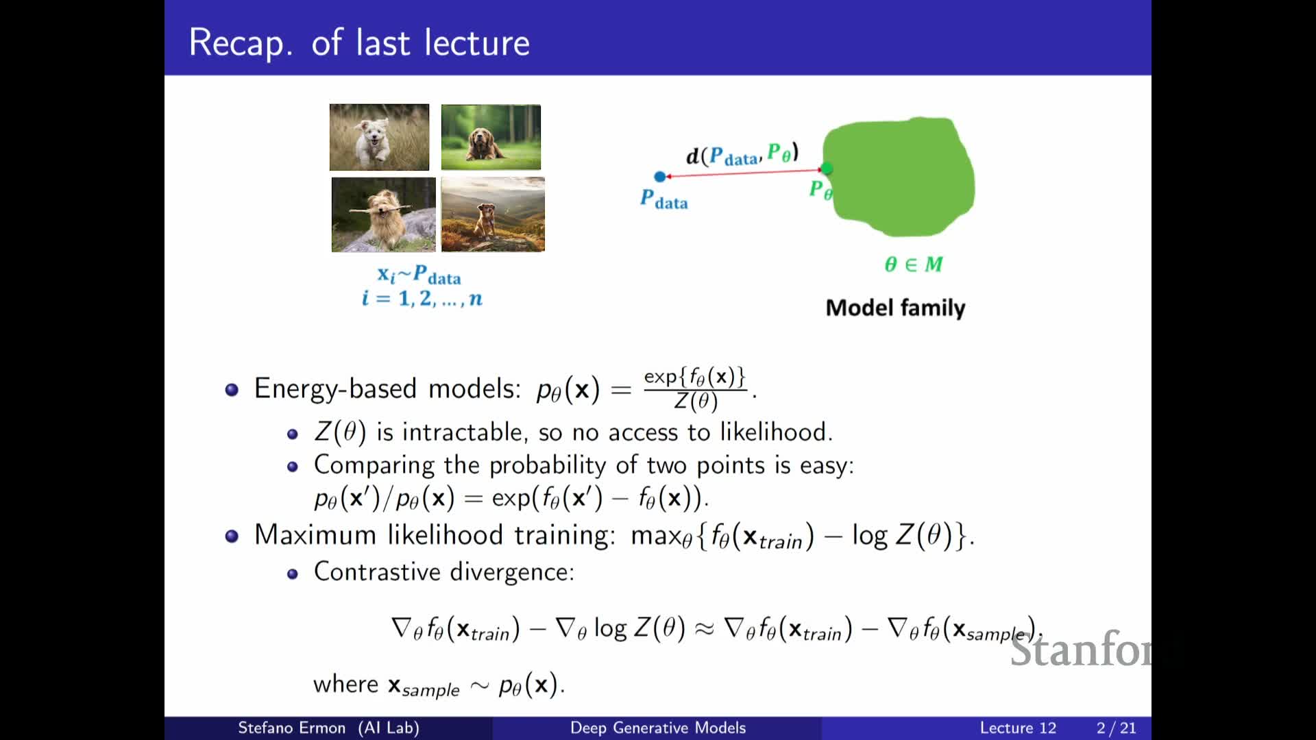
Contrastive Divergence (CD) approximates the log-likelihood gradient by comparing energy gradients at data samples and at samples drawn from the current model, turning the intractable partition-function gradient into a sample-based estimate.
- Start with a minibatch of real data samples.
- Generate short-run samples from the current model (e.g., a few MCMC/Langevin steps) starting from the data or other initializations.
- Compute the gradient difference: increase unnormalized probability (decrease energy) for real data and decrease it for the synthetic samples.
- The intuitive update is: raise mass on data, lower mass on generated samples, approximating the effect of the partition-function term.
- This requires the ability to generate samples from the model; when those samples approximate p_theta well, the CD gradient approximates the true maximum-likelihood gradient.
- Practically, CD shifts complexity from evaluating Z(theta) to generating representative model samples.
Markov chain Monte Carlo (MCMC) methods enable sampling from EBMs via local proposals and acceptance rules that satisfy detailed balance
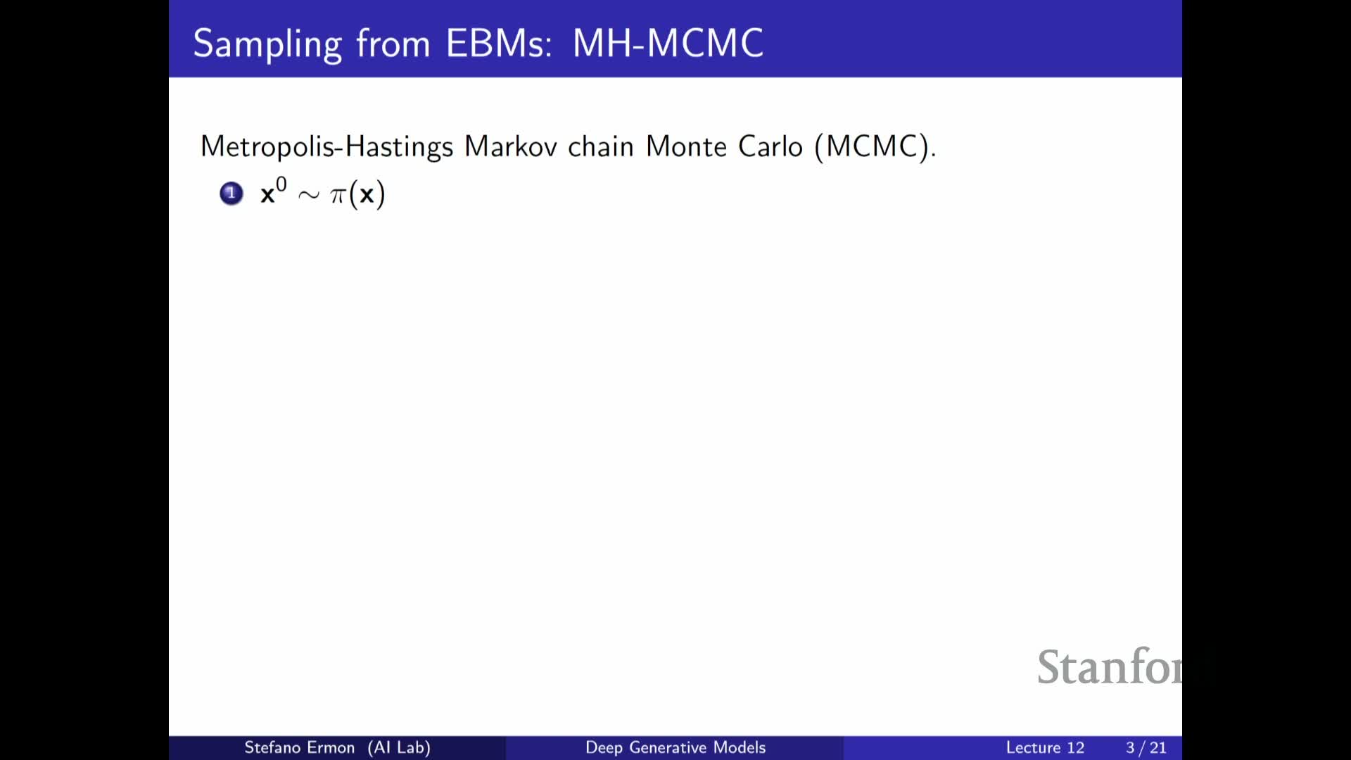
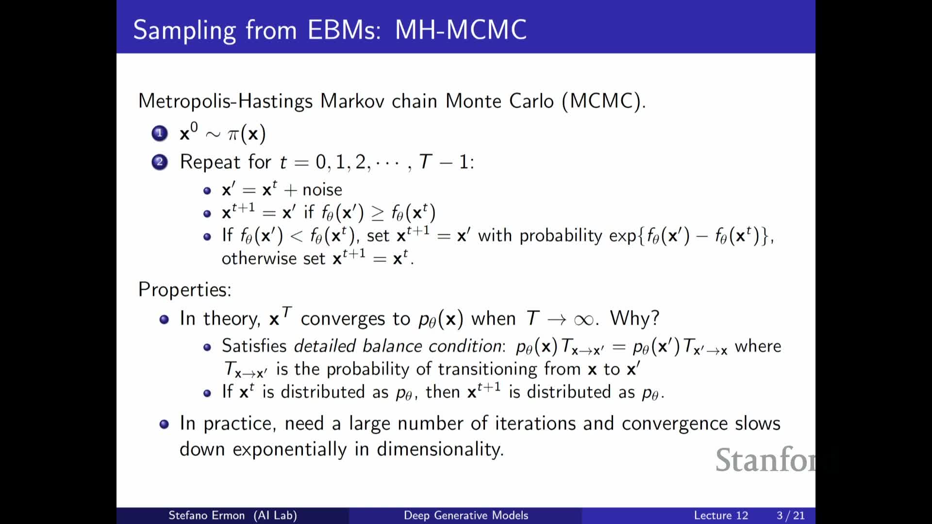
Sampling from an EBM is typically done by constructing a Markov chain whose transition operator satisfies detailed balance with respect to p_theta.
- A common recipe:
- Propose a local perturbation x’ from the current state x.
- Accept or reject x’ based on the ratio of unnormalized probabilities (the Metropolis–Hastings acceptance rule).
- The acceptance rule enforces that transitions occur with probabilities making p_theta a fixed point of the Markov operator, so under mild conditions repeated application converges to p_theta regardless of initialization.
- Intuitively, MCMC is stochastic local search (or stochastic hill-climbing): uphill moves are accepted deterministically, downhill moves accepted with probability proportional to the unnormalized-probability ratio, preserving the correct stationary distribution.
- In high-dimensional spaces, however, mixing can be extremely slow, and many steps may be required to obtain high-quality independent samples.
Langevin dynamics and noisy gradient ascent are efficient MCMC proposals for continuous EBMs using score information
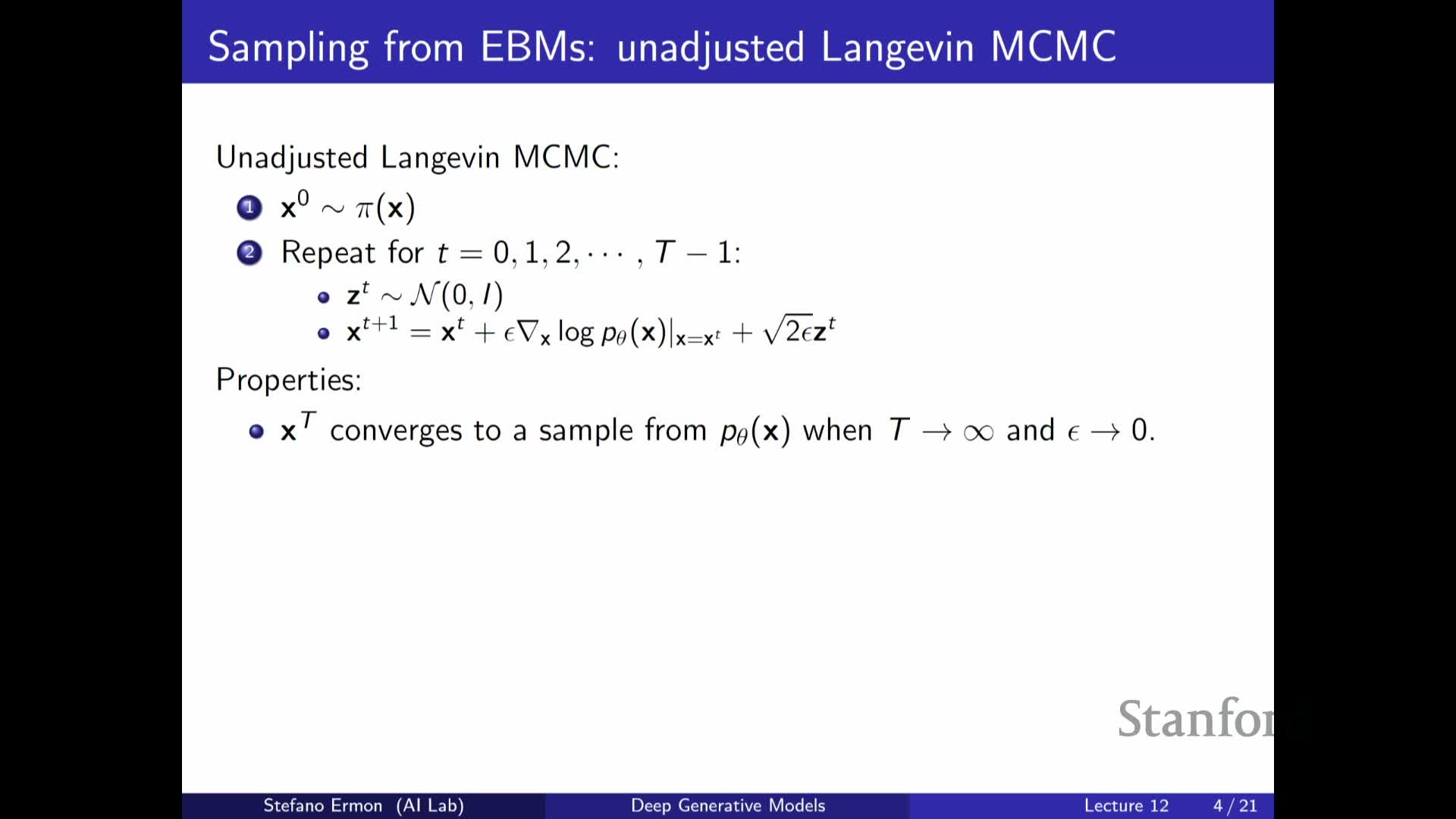
Langevin dynamics perform MCMC in continuous state spaces by combining gradient ascent on the log unnormalized density (the score) with injected Gaussian noise.
- Each update has the form: x_{t+1} = x_t + (epsilon^2 / 2) * grad_x log p_theta(x_t) + epsilon * Normal(0, I), so the step size epsilon controls the signal-to-noise trade-off and must be scaled relative to the gradient magnitude to ensure convergence.
- Variants:
- MALA (Metropolis-adjusted Langevin algorithm) adds an MH accept/reject step to correct discretization bias.
-
Unadjusted Langevin always accepts; both converge to p_theta in the limit of small step size and many iterations under technical conditions.
- Using gradient information (the score) usually yields much faster practical mixing than naive local proposals, but each step is computationally costly because it requires evaluating grad_x f_theta(x) via backprop.
Sampling and contrastive-training costs make naive likelihood-based training of EBMs impractical at scale
Training EBMs with sampling-based inner loops (e.g., CD, MCMC, Langevin) requires generating fresh model samples repeatedly during optimization, which multiplies the cost of forward and backward passes through the energy network by the number of sampling steps.
- If thousands or tens of thousands of sampling steps are needed per sample to reach high-probability modes, including such sampling during each training update becomes computationally prohibitive.
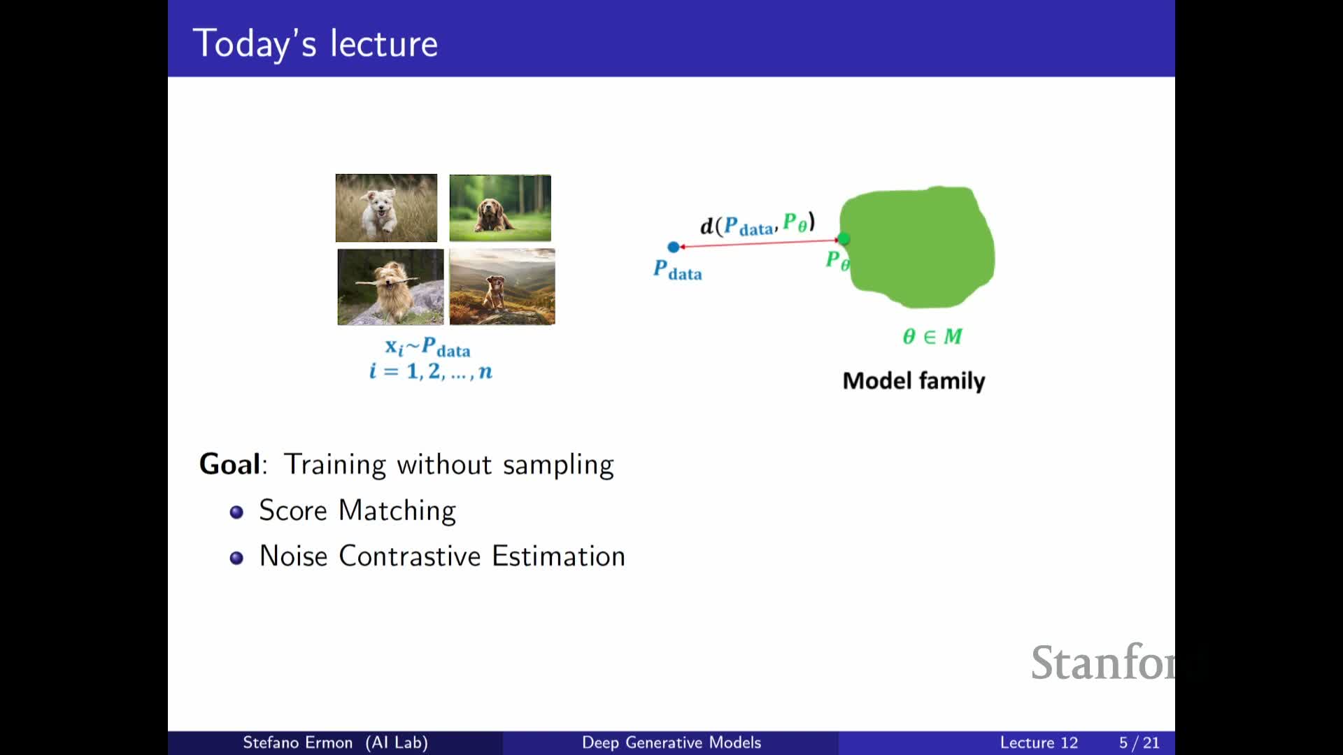
- Therefore, alternative training objectives that avoid model sampling during training are desirable for efficient, scalable EBM training.
- These alternatives typically exploit quantities that do not depend on the partition function.
The score function is the gradient of the log-density with respect to the input and does not depend on the partition function
The score function s_theta(x) = grad_x log p_theta(x) equals grad_x f_theta(x) because the partition function Z(theta) does not depend on x and drops out when differentiating with respect to the input.
- Consequences:
- The score is directly computable from the energy network without evaluating Z(theta).
- It provides a vector field that points in the direction of steepest increase of log-density at every x.
- For simple parametric families (e.g., Gaussians) the score has closed-form dependence on x and parameters; for neural-network energies it is available via automatic differentiation.
- Using the score rather than the log-density itself opens a pathway to construct training losses that avoid partition-function evaluation.
Score matching and the Fisher divergence compare distributions by their score vector fields and yield a partition-free training objective
The Fisher divergence measures discrepancy between two densities p and q by the expected squared L2 norm of the difference between their score functions:
E_{x~p}[ || grad_x log p(x) - grad_x log q(x) ||^2 ], which vanishes iff p = q under mild conditions.
- Because it depends only on score fields, the Fisher divergence does not require evaluating normalization constants, making it well suited to EBMs whose scores are available from the energy gradient.
- Minimizing the Fisher divergence between the data distribution p_data and a model p_theta corresponds to matching their score fields and provides an alternative to KL-based maximum likelihood that is free of explicit partition-function dependence.
- Conceptually, this reframes density matching as aligning a conserved vector field (the score) rather than matching scalar likelihood values.
Integration by parts (and its multivariate analogue) converts the Fisher divergence into a computable loss involving model derivatives only

Although the Fisher divergence contains the unknown data score term, integration by parts (univariate) or the divergence theorem (multivariate) can move derivatives from the unknown data density onto the model score, eliminating explicit dependence on grad_x log p_data under mild boundary conditions.
- In one dimension the manipulation yields an objective composed of:
- The squared model score, and
- The derivative of the model score — both computable for a parametric energy model.
- In multiple dimensions the transformed objective involves:
- The squared norm of the model score, plus
- The trace of the model score’s Jacobian (equivalently, the Hessian of log p_theta).
- Up to a theta-independent constant, the result is an expectation over data samples of terms depending only on the model and its derivatives, enabling empirical estimation by sample averages and stochastic optimization using only training data and energy-network derivatives.
Practical computation of the score-matching loss requires approximations for second derivatives and scalable estimators such as sliced or denoising score matching
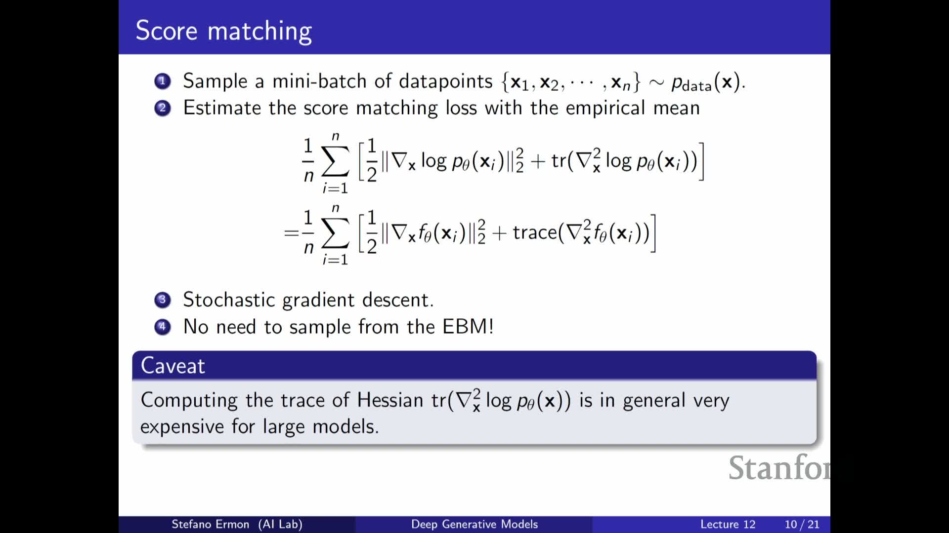
Direct evaluation of the multivariate objective requires computing the trace of the Hessian of log p_theta(x) (or equivalent second-order input derivatives), which is expensive in high dimensions because it naively requires many backward passes.
- Scalable alternatives:
- Hutchinson’s estimator (randomized trace estimation) projects Hessian action onto random vectors to approximate the trace.
- Sliced score matching approximates the multivariate trace via random one-dimensional projections.
-
Denoising score matching recovers score information by training to denoise noisy inputs, avoiding explicit second-order computation.
- Interpreting the resulting loss shows it encourages:
- Data points to be stationary points of the model log-density (small gradients), and
- Those points to be local maxima rather than minima (controlled by second-derivative terms), aligning model mass with data modes.
- These approximations retain the partition-free advantage while enabling practical optimization of score-based objectives at scale.
Noise-contrastive estimation (NCE) trains a classifier to distinguish data from a known noise distribution, yielding density-ratio estimates
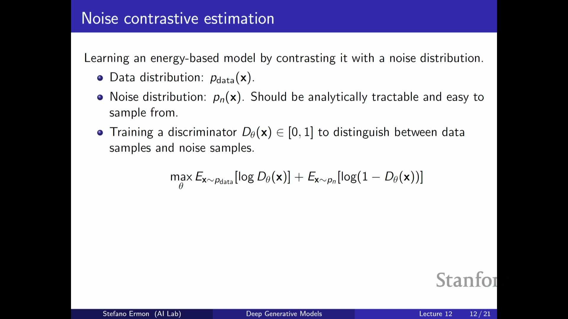
Noise-contrastive estimation (NCE) reframes density estimation as a supervised binary classification problem: a discriminator learns to distinguish real data from samples drawn from a chosen noise distribution p_n(x).
- The optimal classifier recovers the density ratio p_data(x) / (p_data(x) + p_n(x)), so because p_n(x) is chosen to be tractable to sample from and to evaluate, the classifier’s outputs provide information about p_data relative to p_n.
- NCE turns unsupervised density estimation into likelihood-free discriminative training that does not require sampling from the parametric model being trained.
- The choice of noise distribution is critical: when p_n is similar to p_data the classifier must learn subtle structure and yields stronger learning signals.
An energy-based discriminator with a learnable partition constant turns NCE into a trainable EBM without inner-loop sampling
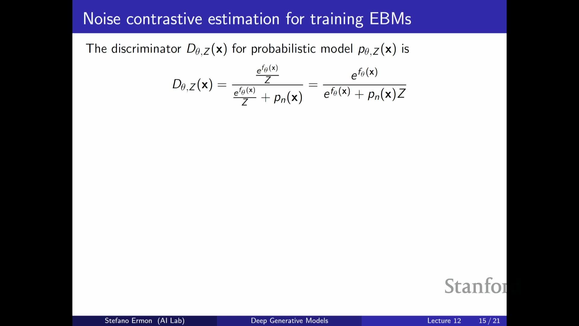
NCE can be specialized to EBMs by parameterizing the classifier’s model likelihood term with p_theta(x) = exp(f_theta(x)) / Z and treating log Z as an additional free scalar parameter z that is optimized jointly with theta.
- Under the cross-entropy objective, optimizing (theta, z) to make the classifier distinguish data from noise pushes p_theta toward p_data in the infinite-data, perfect-optimization limit, and the learned z converges to the true log partition function in that limit.
- Training proceeds by:
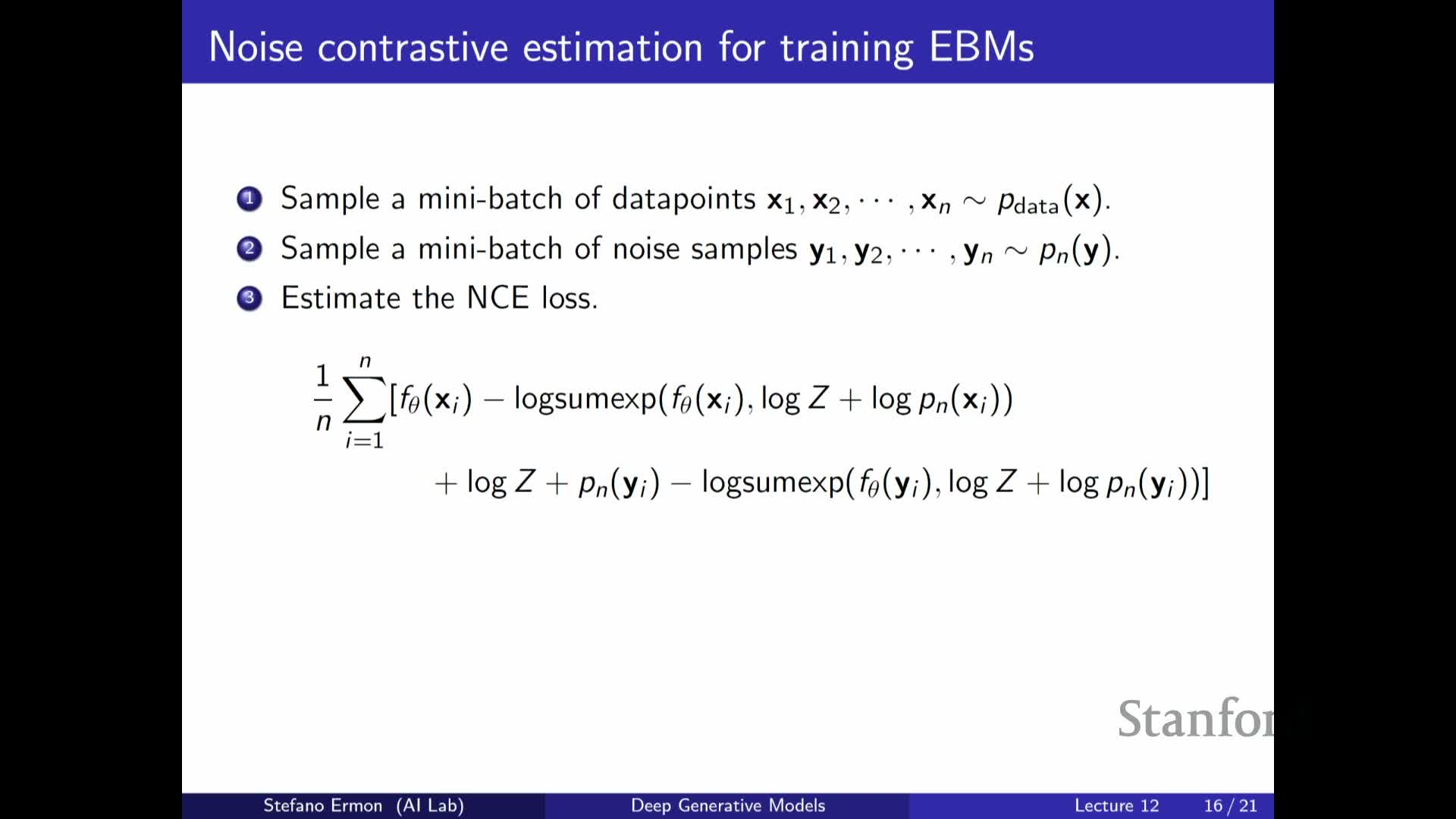
- Sampling minibatches of real data and noise samples from p_n.
- Evaluating the discriminator probability via the energy and the noise density.
- Applying stochastic gradient updates to (theta, z).
- This approach fits EBMs without generating samples from p_theta. In finite-data or imperfect-optimization regimes the learned z may not equal the true partition function, so the energy and normalization are approximate, but NCE remains a practical, likelihood-free fitting method.
Adapting the noise distribution via parametric flows yields flow-contrastive estimation that jointly trains a tractable generator and an EBM-like discriminator
A refinement is to parameterize the noise distribution p_n(x; phi) with a tractable flow model that can both generate samples efficiently and evaluate likelihoods, and to update phi adversarially to make the discriminator’s task harder.
- In flow-contrastive estimation:
- The discriminator (an energy plus normalization scalar) and the flow-based noise model are trained jointly in a minimax-style scheme.
- The flow model is optimized to approximate p_data and confuse the discriminator, while discriminator updates push the energy toward p_data.
- This yields two learned objects—a flow generator and an energy function—and in practice the flow can provide high-quality samples while the energy captures discriminative density structure.
- The approach bridges score-based, contrastive, and adversarial paradigms but requires careful tuning due to the adversarial component. Empirically, learning the noise distribution often improves sample quality compared to a fixed noise distribution, while theoretical guarantees revert to the infinite-data, perfect-optimization limits.
Enjoy Reading This Article?
Here are some more articles you might like to read next: