Stanford CS236- Deep Generative Models I 2023 I Lecture 13 - Score Based Models
- Course overview and motivations for score-based generative models
- Definition and interpretation of the score function
- Energy-based models and score matching motivation
- Modeling scores directly as vector-valued neural networks
- Statistical considerations and overfitting when learning scores from samples
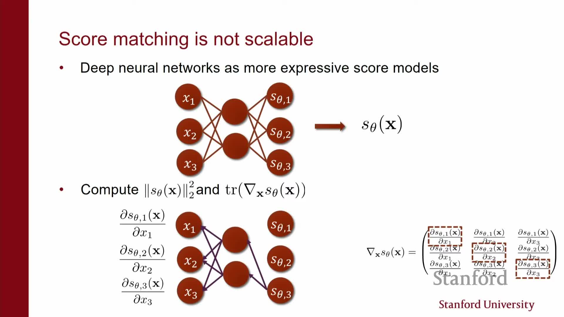
- Score-matching objective, integration by parts, and computational bottleneck
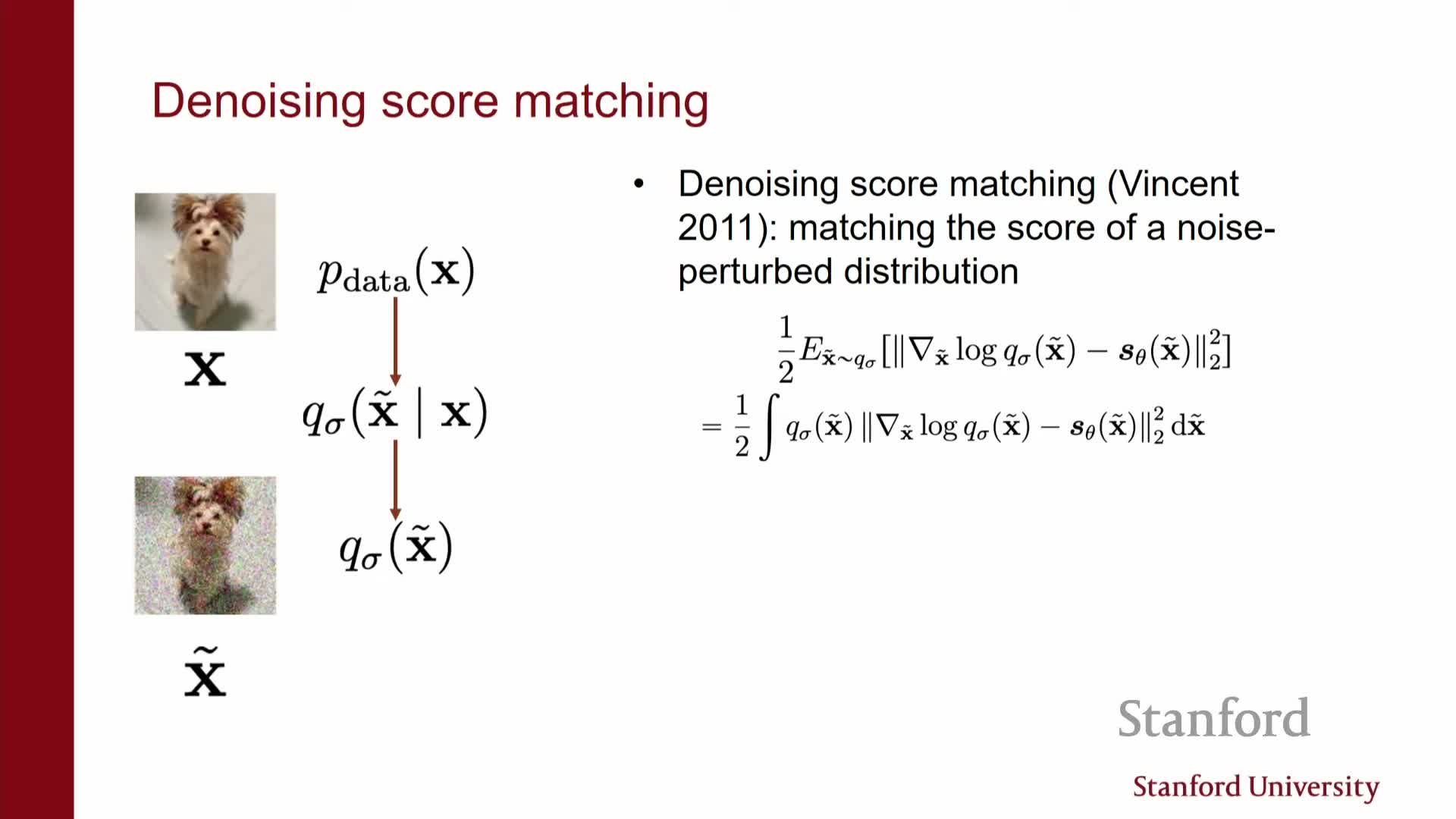
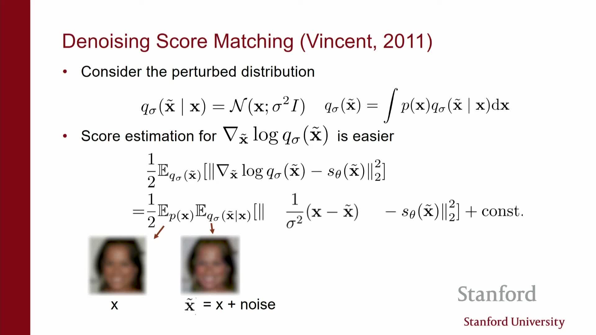
- Denoising score matching concept and noise-perturbed densities
- Algebraic transformation from Fisher divergence to denoising objective
- Denoising objective interpretation and practical algorithm
- Tweedie formula, conditional expectation, and implications for denoising
- Sliced (random-projection) Fisher divergence for scalable exact score matching
- Sampling with estimated scores via Langevin dynamics and MCMC
- Failure modes: data manifolds and low-density regions causing poor sampling and mixing
- Conclusion: limitations of naive score matching and path to diffusion models
Course overview and motivations for score-based generative models
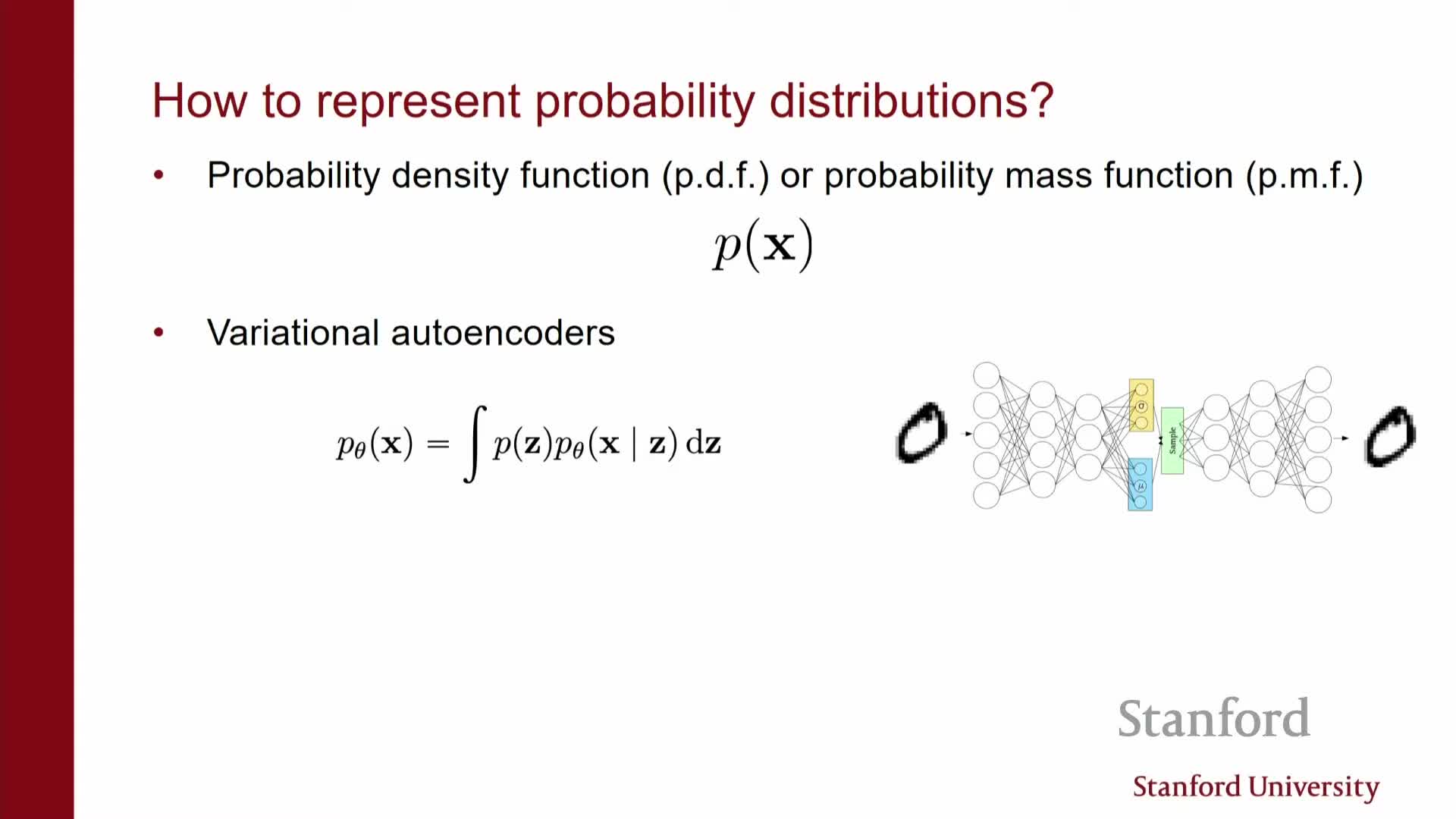
This segment defines the landscape of modern generative modeling and motivates score-based approaches.
-
Likelihood-based models (e.g., autoregressive models, normalizing flows) require explicit normalized densities and enable principled likelihood training and monitoring.
-
Implicit generator models define flexible sampling procedures but make likelihood evaluation intractable, so they rely on adversarial or other unstable training methods.
Trade-offs:
- Likelihood models: principled training and easy evaluation, but they impose architectural constraints.
- Implicit models: high flexibility, but need unstable or complex training (e.g., GANs).
This motivates score-based (diffusion) models: instead of modeling the density itself, they model the gradient of the log density — the score — which avoids explicit normalization while allowing flexible parameterizations for continuous data modalities.
Definition and interpretation of the score function

Score function: the gradient of the log probability density with respect to the input, ∇_x log p(x).
- Geometric interpretation: the score is a vector field that points in the direction of greatest increase of log density at each input location — it encodes local directions toward higher-probability regions.
- Working with the score removes the explicit normalization constraint because gradients eliminate additive constants in the log density.
- This is computationally attractive when densities exist for continuous random variables.
Analogy: think of potentials (log density / energy) versus fields (score) — equivalent information up to constants, but the field representation avoids partition-function issues and can be more convenient for some tasks.
Energy-based models and score matching motivation
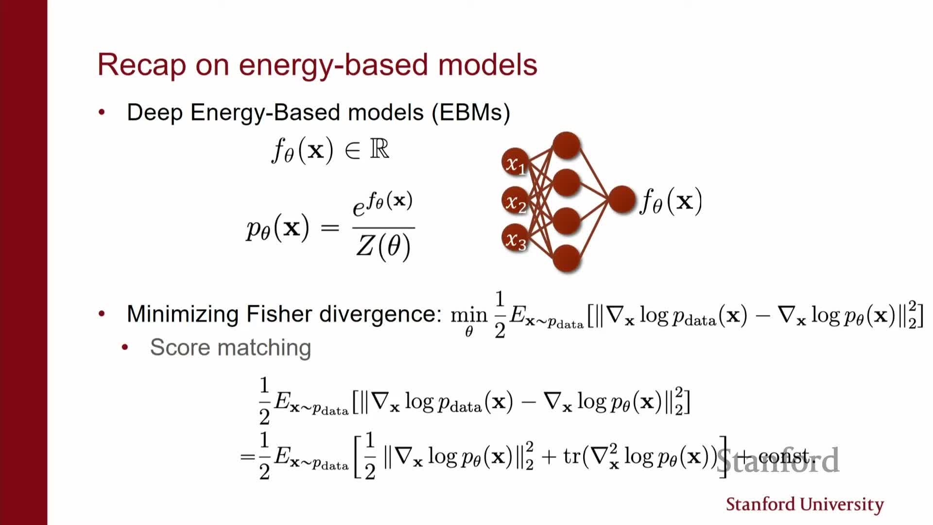
This segment positions score-based modeling relative to energy-based models (EBMs) and introduces the Fisher divergence as a training objective.
-
EBMs parameterize an unnormalized energy and face partition-function estimation difficulties when trained by likelihood.
-
Crucially, the score (the gradient of the energy) does not depend on the partition function, so matching scores avoids normalization issues.
-
Fisher divergence: the expected squared difference between data and model scores.
- Via integration by parts, the Fisher objective can be rewritten so it does not require computing the partition function explicitly.
- This motivates score matching as a tractable alternative for fitting flexible unnormalized models.
- Via integration by parts, the Fisher objective can be rewritten so it does not require computing the partition function explicitly.
Modeling scores directly as vector-valued neural networks
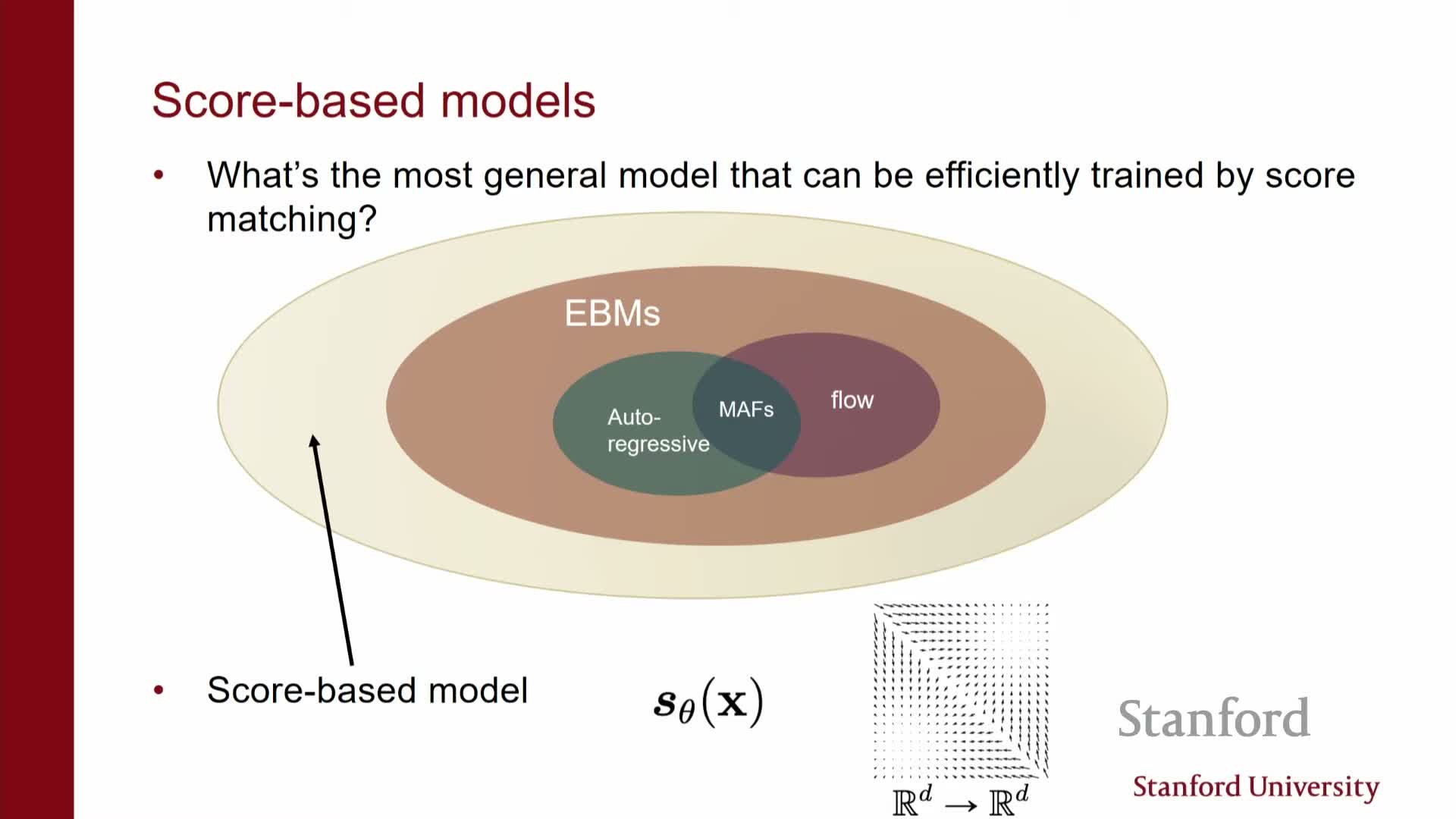
Core modeling choice in score-based methods:
- Parameterize the score directly as a vector-valued neural network s_theta(x) mapping R^d → R^d.
- The model family becomes a set of vector fields obtained by varying network parameters; each output vector matches the input dimensionality because it represents a gradient.
- Training objective: find parameters that make the model vector field close to the data score vector field in a suitable norm, using only samples from the data distribution.
This formulation generalizes EBMs by not requiring that the modeled vector field be the gradient of a scalar potential (i.e., the field need not be conservative).
Statistical considerations and overfitting when learning scores from samples

Learning-theoretic and practical issues with finite samples:
- Training from samples turns score matching into an empirical risk minimization problem subject to standard concerns: sample complexity, estimation error, and overfitting.
- Matching scores everywhere is limited by finite data and model capacity; derivative information (scores) contains the same information as densities up to a normalization constant, so estimation remains challenging.
- Conceptual difference: modeling an energy (a scalar potential) versus modeling a vector field directly.
- Direct score models can represent non-conservative fields that an energy parameterization cannot.
- Direct score models can represent non-conservative fields that an energy parameterization cannot.
Score-matching objective, integration by parts, and computational bottleneck
This segment derives the Fisher-divergence training objective and explains the computational bottleneck.
-
The empirical objective is E_data[ s_theta(x) − s_data(x) ^2].
- Integration by parts rewrites this into a form depending only on model outputs and their derivatives with respect to inputs.
- The problematic term is the trace of the Jacobian (sum of ∂(s_theta)_i / ∂x_i), which, if computed naively, requires O(d) backpropagations and becomes intractable in high-dimensional data.
Denoising score matching concept and noise-perturbed densities
This segment introduces denoising score matching as a scalable approximation that sidesteps computing Jacobian traces.
- Key idea: convolve the data distribution with a known noise kernel (commonly Gaussian) to obtain a smoothed density Q_sigma whose score is easier to estimate.
- Training targets the score of this noise-perturbed distribution instead of the original data score.
- The learning objective for the smoothed density can be rewritten into an efficient denoising loss, eliminating the intractable trace term.
- If the added noise level is small, Q_sigma approximates the original data distribution, so learning the noisy score yields a useful approximation of the clean score.
Algebraic transformation from Fisher divergence to denoising objective
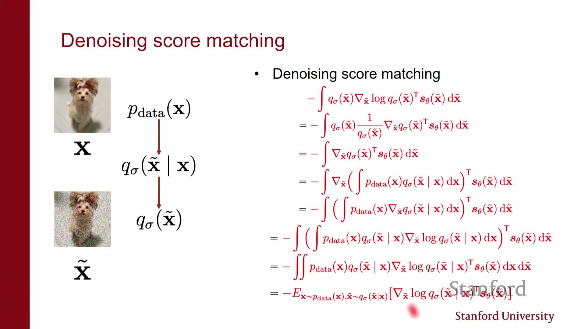
This segment sketches the algebraic steps that convert the Fisher objective on the noisy distribution into a tractable denoising loss.
- Write the noisy marginal Q_sigma(x_tilde) as an integral over clean data x and exchange gradients with the integral.
-
The intractable dependence on the unknown data score disappears and is replaced by gradients of the conditional noise kernel p(x_tilde x).
- For a Gaussian kernel these conditional-score terms have closed-form expressions (linear in x_tilde − x), so the troublesome cross-term simplifies to an expectation involving known quantities and the model output.
- The end result is a computable squared-error denoising loss that depends only on samples (x, x_tilde) and the model’s output at x_tilde.
Denoising objective interpretation and practical algorithm
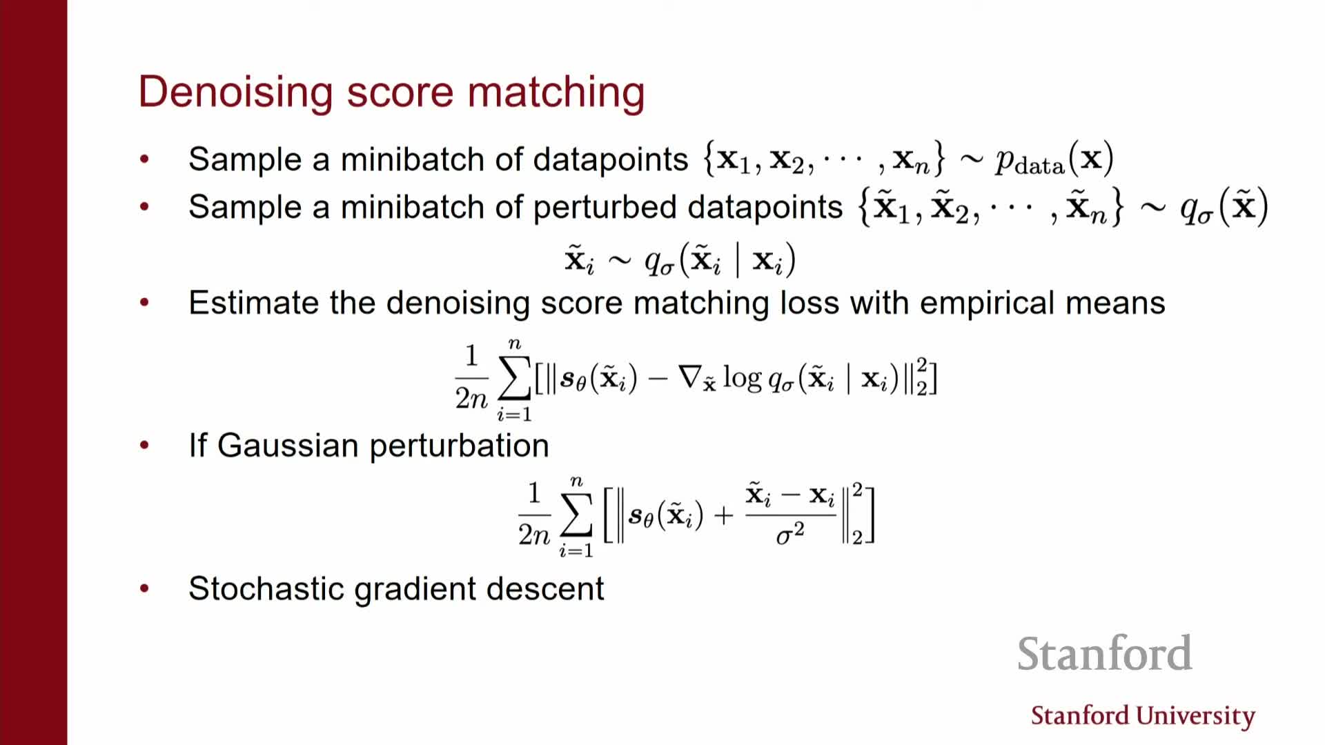
Final denoising loss form and practical training algorithm:
- For Gaussian perturbations the loss reduces to an L2 regression objective: train s_theta(x_tilde) to predict the noise vector (x_tilde − x) scaled by the inverse variance (or equivalently predict the score of the noisy density).
Practical mini-batch training algorithm (per update):
- Sample clean data x from the dataset.
- Sample noise eps ∼ N(0, σ^2 I) and form x_tilde = x + eps.
- Compute the denoising target (e.g., eps / σ^2 or the equivalent score target) and evaluate the squared-error loss between model output s_theta(x_tilde) and the target.
- Update θ by minimizing the empirical denoising loss (standard gradient-based optimizer).
-
Sigma trade-off: smaller σ yields a closer approximation to the clean score but can cause numerical instability or poor conditioning; in practice one picks or schedules multiple σ values to balance accuracy and stability.
Tweedie formula, conditional expectation, and implications for denoising
Statistical rationale behind denoising score matching using Tweedie’s formula and conditional expectations:
-
For additive Gaussian noise, the MMSE denoiser E[x x_tilde] is related to the gradient of the log-perturbed density by a closed-form relation (Tweedie’s formula).
- Minimizing the L2 denoising loss implicitly aligns the model with the noisy-score direction that points toward high-probability clean images.
- Other noise kernels can be used provided their conditional scores are computable, but Gaussian noise yields particularly simple expressions and theoretical guarantees that are convenient in practice for sampling and score estimation.
Sliced (random-projection) Fisher divergence for scalable exact score matching
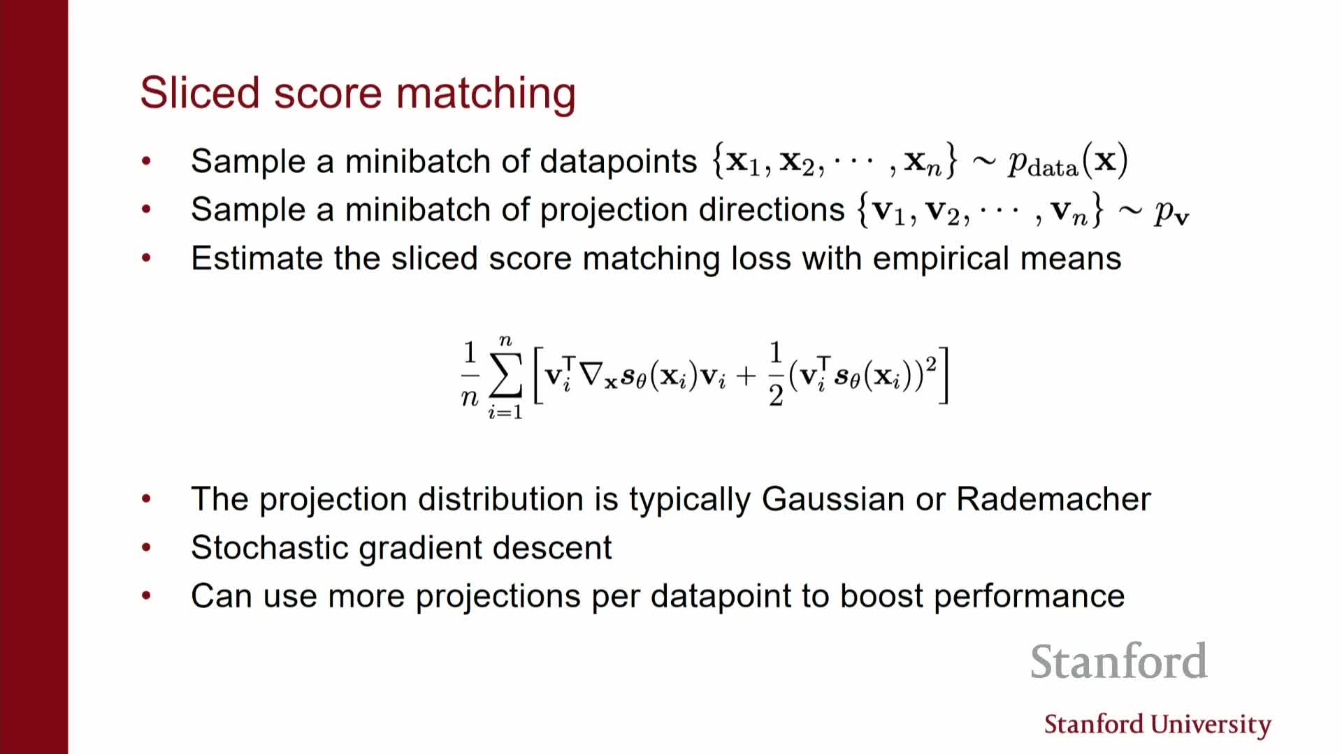
This segment presents an alternative scalable approach: sliced score matching (projecting onto random directions).
- Project the vector-valued score s(x) onto random directions v and match scalar projections v^T s(x) instead of the full vector field.
- The sliced Fisher divergence compares these projections; integration by parts still applies and the problematic trace term reduces to Jacobian-vector products (directional derivatives).
- Jacobian-vector products can be computed with a single backpropagation using standard automatic differentiation, making this approach computationally cheap.
- Sampling random directions per data sample yields unbiased estimators of the full objective; variance is controllable by averaging multiple projections per sample.
Sampling with estimated scores via Langevin dynamics and MCMC
This segment explains how to generate samples when only the score is available, using Langevin dynamics.
- Langevin sampling alternates two steps repeatedly:
- take a small step in the direction of the estimated score (approximate gradient ascent on log density), and
- add Gaussian noise to inject stochasticity.
- take a small step in the direction of the estimated score (approximate gradient ascent on log density), and
- In the limit of vanishing step size and many iterations, Langevin dynamics recovers samples from the target distribution when the score estimator is accurate.
- Important caution: pure gradient ascent without noise leads to mode-seeking and poor diversity; Langevin dynamics combines gradient guidance with stochasticity to approximate the correct stationary distribution.
Failure modes: data manifolds and low-density regions causing poor sampling and mixing
Practical failure modes of score-based sampling and their causes:
-
Data concentrated on low-dimensional manifolds: the score may blow up or be undefined off the manifold, causing unstable or meaningless gradients away from the data support.
-
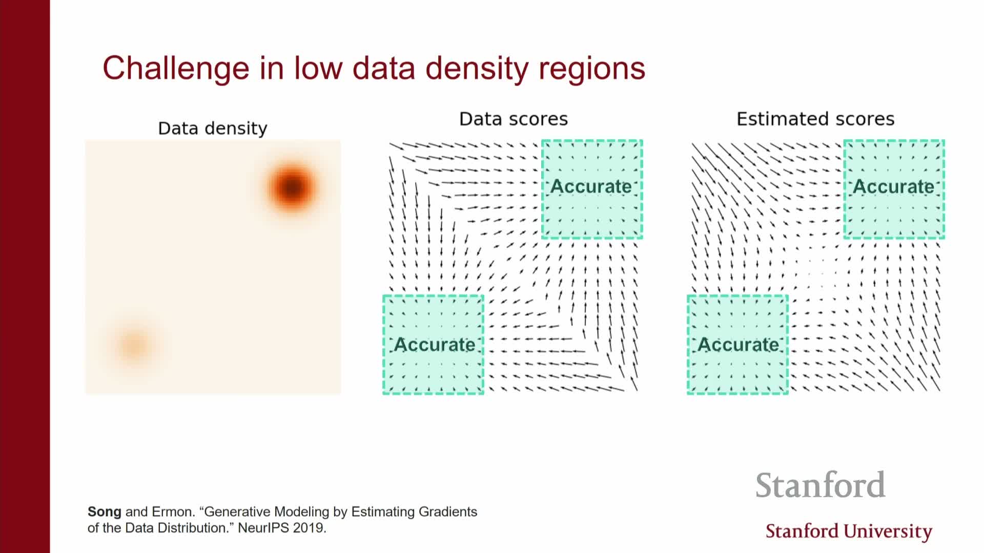
Poor score estimates in low-density regions: finite-data training yields accurate scores only near high-density regions, leaving large gaps with unreliable estimates.
- Consequences for Langevin sampling:
- Failure to reach or mix between modes.
- Misrepresentation of mode probabilities (e.g., mixtures with disjoint supports where the score does not encode mixture weights).
- Failure to reach or mix between modes.
- These issues lead to degraded sample quality and limited exploration unless addressed by improved training or model design.
Conclusion: limitations of naive score matching and path to diffusion models
Summary and practical outlook:
- Direct score modeling and its scalable variants (denoising, sliced) resolve partition-function issues and reduce computational cost compared to naive EBM likelihood training.
- However, naive application is insufficient for high-dimensional real data because of manifold effects and poor estimation in low-density regions.
- Reliable score estimation across the input space requires improved training procedures and architectures (e.g., multi-scale noise schedules, better samplers).
- In practice, diffusion-model techniques that combine careful noise scheduling and enhanced sampling procedures address these challenges and achieve state-of-the-art generative performance, positioning diffusion-based sampling plus robust score estimation as the practical solution to the issues identified.
Enjoy Reading This Article?
Here are some more articles you might like to read next: