Stanford CS236- Deep Generative Models I 2023 I Lecture 14 - Energy Based Models
- Score-based models represent probability distributions via neural network parameterized score vector fields
- Denoising score matching trains the score model on noise-perturbed data rather than the clean data distribution
- Slice score matching uses random one-dimensional projections to make score estimation scalable while targeting the true data score
- Langevin dynamics uses the score field for sampling but fails in practice on high-dimensional manifold-supported data
- Adding noise to data remedies manifold and low-density problems by giving the perturbed distribution full support
- The data manifold concept explains why noise magnitude matters and motivates a tradeoff between estimation accuracy and target mismatch
- Diffusion / score-based models jointly learn scores at multiple noise levels and sample by annealing from high to low noise
- A single noise-conditional neural network amortizes estimation across many noise levels and balances model capacity and efficiency
- Training uses a weighted mixture of denoising objectives across noise scales and often parameterizes outputs as noise predictors
- Training is implemented by stochastic gradient descent with per-sample noise-level selection and amortized denoising tasks
- Sampling uses annealed Langevin dynamics or numerical solvers of reverse-time SDEs, with tradeoffs between steps and sample quality
- The continuous-time diffusion perspective formulates forward corruptions as an SDE and sampling as solving a reverse-time SDE conditioned on scores
- Diffusion models connect to deterministic ODEs and continuous normalizing flows, and exhibit strong empirical performance with memorization caveats
Score-based models represent probability distributions via neural network parameterized score vector fields
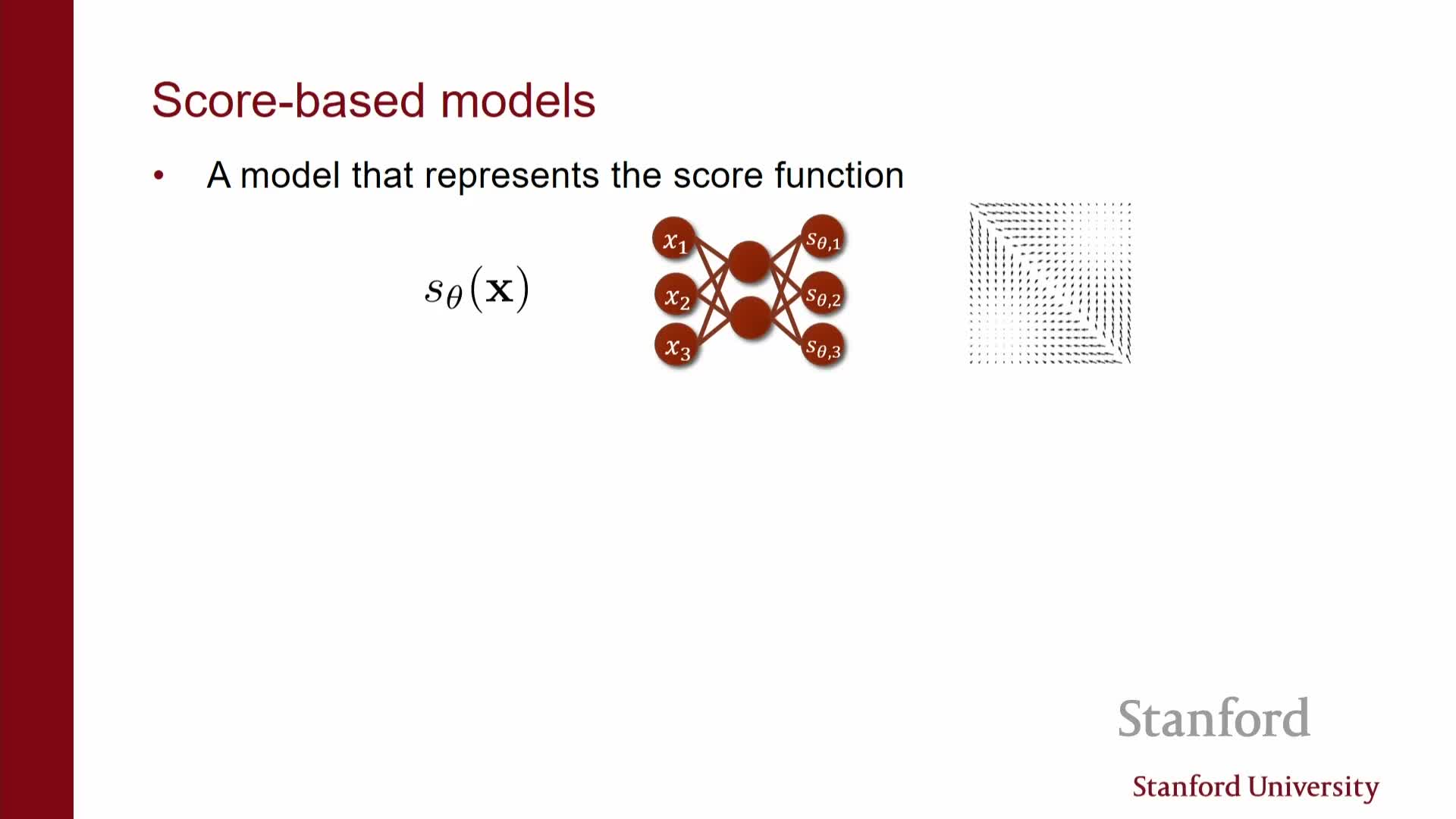
Score-based models parameterize the gradient of the log-density—the score—as a vector-valued neural network that maps each point in data space to the local gradient of log probability.
- The model output is a vector field s_theta(x) intended to approximate ∇_x log p_data(x).
- Training seeks to make that vector field match the true score field.
-
Score matching provides a principled loss for fitting this vector field by minimizing an expectation derived via integration by parts.
- The direct objective, however, involves the trace of a Jacobian, which is computationally prohibitive in high dimensions.
Consequently, naive score matching is impractical for image-scale problems without scalable approximations or alternative formulations.
Denoising score matching trains the score model on noise-perturbed data rather than the clean data distribution
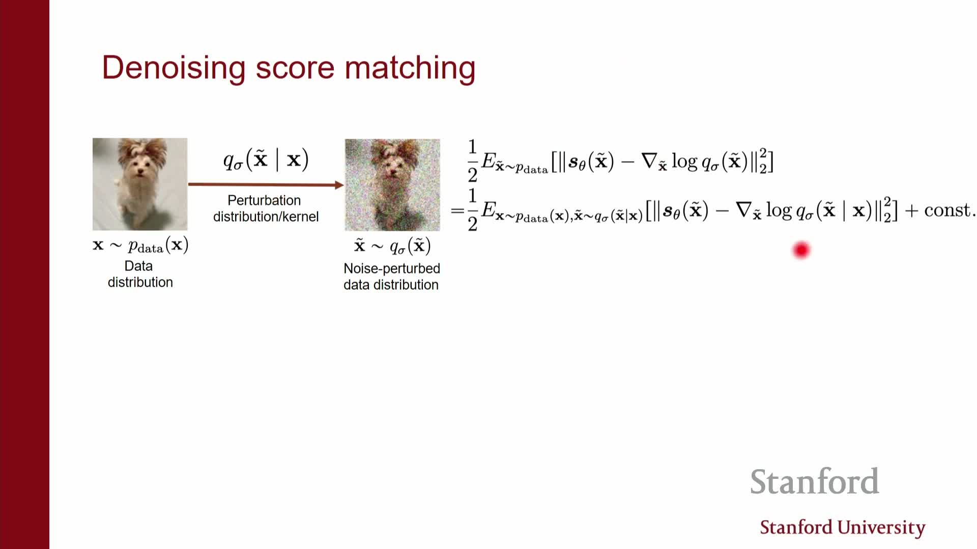
Denoising score matching (DSM) learns the score of a noise-perturbed data distribution q_sigma(x_t | x) obtained by adding noise (typically Gaussian) to a clean data point x.
- Instead of estimating ∇ log p_data(x) directly, DSM trains the network to predict the score of the corrupted distribution, ∇_x log q_sigma(x_t).
- This can be implemented as a simple regression objective (e.g., L2 loss) between the network output and the tractable score of the perturbation kernel.
- For Gaussian perturbations the score has a closed-form expression proportional to the difference between the corrupted input and the clean mean, yielding an efficient per-sample training target and removing the need to compute Jacobian traces.
DSM is computationally scalable, compatible with common neural architectures, and admits a natural denoising interpretation: the network learns to recover the added noise or the clean signal as a function of noise level.
Slice score matching uses random one-dimensional projections to make score estimation scalable while targeting the true data score
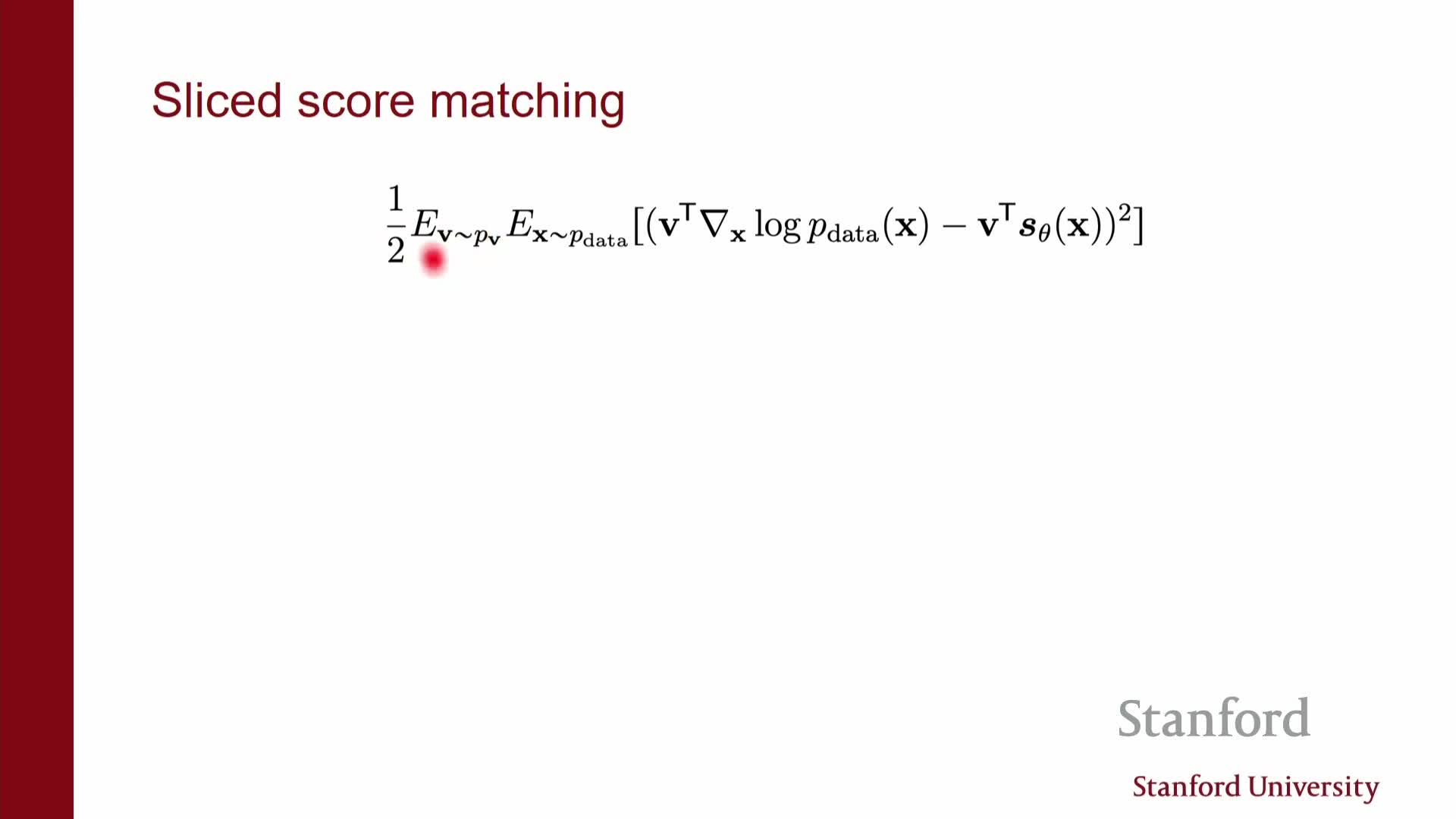
Slice score matching projects the vector-valued score at each point along randomly sampled directions v and matches scalar projections rather than full gradients.
- At each sample the method draws a random direction v and computes the projected scalar score ⟨v, ∇_x log p(x)⟩.
- The model is trained to match that scalar via an objective that can be rewritten to depend only on the model using integration by parts.
- This replaces full Jacobian computations with directional derivatives, which are far cheaper to compute.
Compared to DSM: slice score matching directly targets the score of the clean data distribution (no corruption), but it still requires derivative computations and is somewhat slower in practice.
When the true-data score is well defined, slice score matching yields consistency with that score.
Langevin dynamics uses the score field for sampling but fails in practice on high-dimensional manifold-supported data
Langevin dynamics integrates noisy gradient ascent on log-density using the learned score field: x_{t+1} = x_t + α s_theta(x_t) + √(2α) ξ.
- The scheme moves particles toward high-probability regions by combining score-driven updates with injected noise.
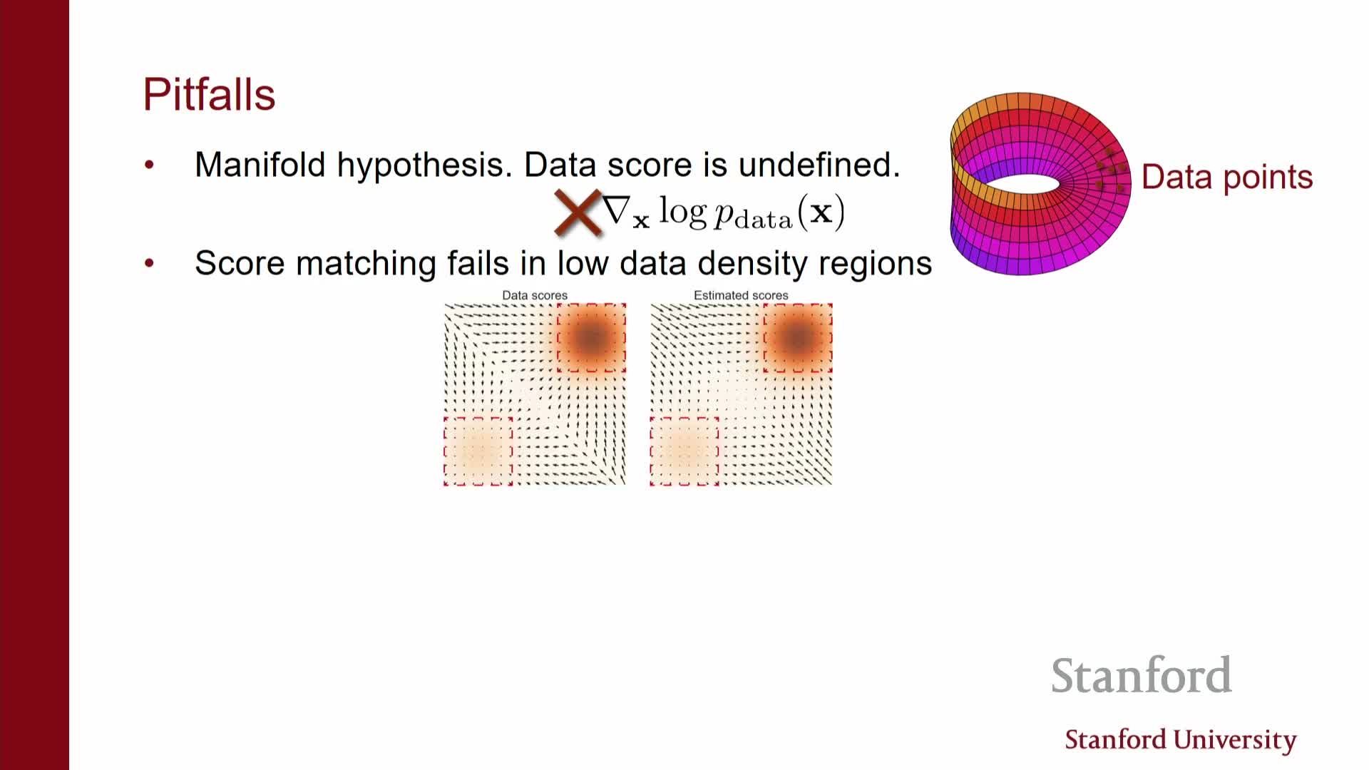
- It assumes well-defined scores away from training samples, but natural-image data typically lies on or near a low-dimensional manifold in pixel space where the score can be ill-defined or explode off the manifold.
- Learned scores are most accurate near high-density training regions and unreliable in low-density regions.
- As a result, naive Langevin chains can get lost, mix poorly between modes, and fail to converge to realistic samples.
These limitations motivate strategies to make score estimation more robust off the data manifold and to improve mixing during sampling.
Adding noise to data remedies manifold and low-density problems by giving the perturbed distribution full support

Convolving the data distribution with isotropic noise (e.g., Gaussian) produces a family of noise-perturbed densities that have full support in ambient space, eliminating singular manifold support and producing well-defined, bounded scores everywhere.
- Estimating scores for these perturbed densities is empirically easier and yields smoother loss landscapes: small Gaussian noise regularizes the score estimation problem and improves optimization stability.
- The tradeoff is that the learned score corresponds to the perturbed (noisy) distribution, so following that score naively produces noisy samples rather than clean data.
This motivates either methods to denoise samples after sampling or learning scores across multiple noise scales so sampling can transition from very noisy to nearly clean distributions.
The data manifold concept explains why noise magnitude matters and motivates a tradeoff between estimation accuracy and target mismatch

Real data typically occupy a low-dimensional embedded manifold in high-dimensional observation space.
- Many pixel combinations thus have essentially zero probability under p_data, and ∇ log p_data can be ill-behaved off the manifold.
- Adding a small amount of noise smooths the distribution and eases estimation near the manifold, but:
- Very small noise does not resolve low-density estimation far from data.
- Very large noise destroys the signal needed to recover clean samples.
- Very small noise does not resolve low-density estimation far from data.
There is an inherent tradeoff: increasing noise improves global score estimation and mixing but moves the learned target away from p_data; decreasing noise yields a score closer to the true data score but is harder to estimate and leads to poor mixing.
This tension motivates methods that jointly consider multiple noise magnitudes rather than a single perturbation scale.
Diffusion / score-based models jointly learn scores at multiple noise levels and sample by annealing from high to low noise
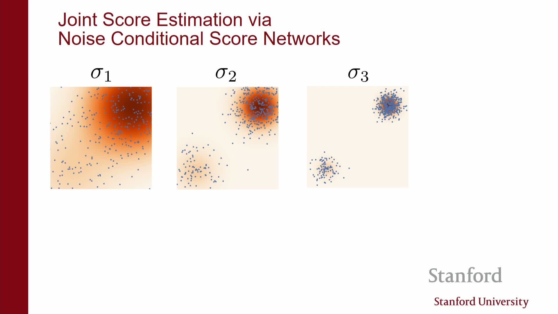
Diffusion / score-based models estimate score fields for a sequence of noise scales σ_L, …, σ_1 that interpolate between heavy corruption and near-clean data.
- Sampling starts from essentially pure noise and then sequentially applies a sampling procedure (e.g., annealed Langevin dynamics) that:
- Uses the score for a large-noise level to obtain reasonably mixed initial particles.
- Progressively switches to scores for smaller noise levels to introduce finer structure.
- Uses the score for a large-noise level to obtain reasonably mixed initial particles.
- The multiscale strategy yields accurate directional information at all stages: coarse scales guide global structure and mixing, while fine scales refine details, enabling generation of nearly clean samples despite estimation challenges at any single noise level.
Practical implementations discretize a continuum of noise levels (often ~1000 steps) and amortize computation by conditioning one neural network on the noise level.
A single noise-conditional neural network amortizes estimation across many noise levels and balances model capacity and efficiency
Training a separate score network for each noise scale is computationally costly, so practice uses a single noise-conditional network s_theta(x, σ) that takes the noise scale σ (or time index) as an additional input and jointly approximates scores for all desired corruptions.
- This network shares computation and parameters across scales, amortizing learning.
- Implementation choices include embedding σ and concatenating or injecting it via adaptive layers.
- The resulting vector fields are not required to be conservative (exact gradients of an energy), although conservative parameterizations are possible; empirically, free-form vector fields perform well.
Key hyperparameters: the number of discrete noise levels, maximum and minimum magnitudes, and the interpolation schedule (commonly geometric), which control overlap between successive noise shells and the success of annealed sampling.
Training uses a weighted mixture of denoising objectives across noise scales and often parameterizes outputs as noise predictors
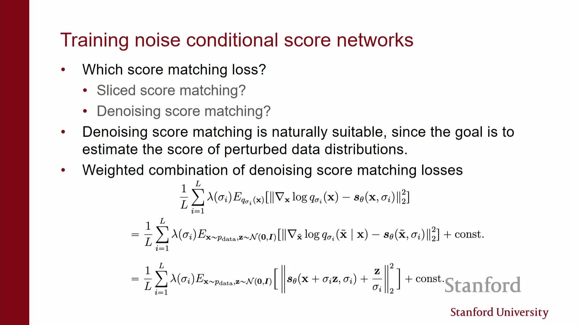
The training objective sums or integrates denoising score-matching losses over the chosen noise scales and typically weights each term with a function λ(σ) that balances contributions by noise magnitude and numerical conditioning.
- For Gaussian perturbations a convenient parameterization is to predict the added noise ε (using ε_theta) from the corrupted input x_t; this noise-prediction parameterization is algebraically equivalent to predicting the scaled score and often improves numerical stability.
- The loss is implemented by:
- Sampling a mini-batch of clean data.
- Sampling σ (or an index) per example and generating noisy inputs x_t = x + σ ε.
- Minimizing the weighted squared error between predicted and true noise (or between predicted and true score).
- Sampling a mini-batch of clean data.
- Proper choice of λ(σ) or scaling factors ensures no single noise level dominates training and yields balanced performance across scales.
Training is implemented by stochastic gradient descent with per-sample noise-level selection and amortized denoising tasks
Each training iteration proceeds as follows:
- Sample a batch of data points.
- For each point, independently sample a noise scale σ (commonly uniformly or according to a prescribed schedule).
- Draw Gaussian noise and form the corrupted input x_t = x + σ ε.
- Evaluate the network s_theta(x_t, σ) or ε_theta(x_t, σ) and compute the per-sample denoising regression loss weighted by λ(σ).
- Backpropagate gradients and update parameters with standard optimizers (SGD/Adam).
This single-model, multi-task setup amortizes the cost of solving many denoising tasks and yields a model usable at inference across all noise scales.
In practice, practitioners discretize σ levels (e.g., 1000) and may optionally ensemble or use multiple networks for incremental gains if compute permits.
Sampling uses annealed Langevin dynamics or numerical solvers of reverse-time SDEs, with tradeoffs between steps and sample quality

Sampling from the model begins from samples of a high-noise prior (essentially Gaussian) and iteratively reduces noise by running a stochastic procedure that uses s_theta(x, σ) to push particles toward higher-density regions while injecting appropriate noise at each step.
-
Annealed Langevin dynamics applies multiple Langevin updates at each discrete σ, using the corresponding conditional score and optionally decreasing step sizes. More steps yield higher quality but increase inference cost because each step requires a full model evaluation.
- Viewing the noise sequence as a discretization of a continuous diffusion process leads to reverse-time SDEs whose numerical integration (predictor-corrector methods) provides principled solvers and can be combined with Langevin correctors for improved mixing.
The practical tradeoff is compute versus fidelity: state-of-the-art models often use thousands of network evaluations to generate very high-quality images, which is far more expensive at inference than alternative generator architectures but produces superior results and stable training behavior.
The continuous-time diffusion perspective formulates forward corruptions as an SDE and sampling as solving a reverse-time SDE conditioned on scores
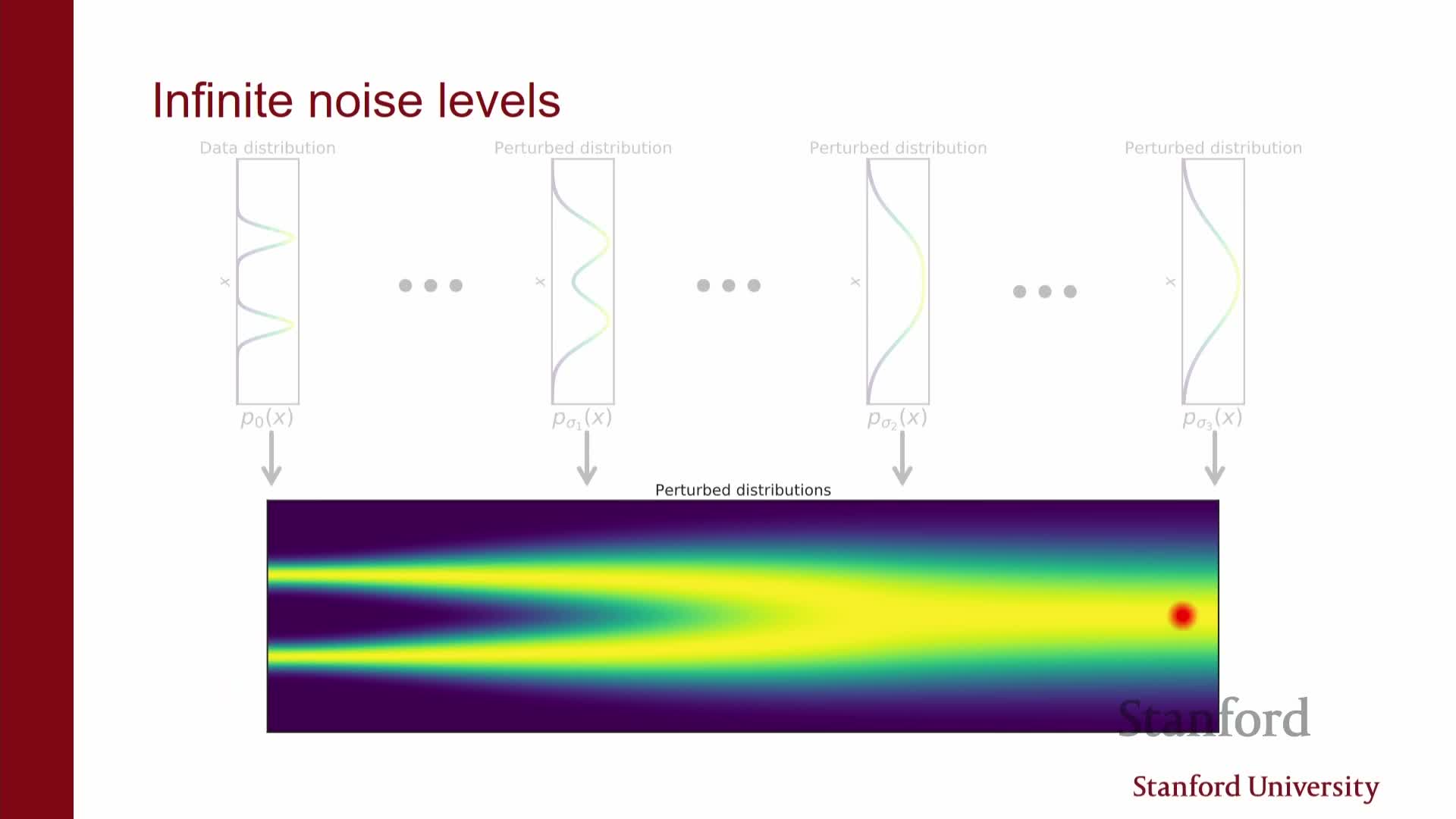
A continuum of noise levels is naturally modeled as a stochastic process {x_t}_{t∈[0,T]} obtained by an SDE that gradually corrodes data into noise; the marginal at each time t corresponds to the data distribution convolved with the appropriate Gaussian.
- Reversing time yields a reverse-time SDE whose drift term depends on the score ∇_x log p_t(x), so accurate score estimates across t allow construction of an exact generative reverse-time dynamics.
- Replacing the true score by s_theta(x, t) yields a tractable reverse SDE that can be numerically integrated with standard SDE solvers; discretization recovers annealed sampling procedures.
- This SDE viewpoint clarifies connections to classical diffusion theory and enables use of advanced numerical techniques (higher-order solvers, predictor-corrector steps) to trade off step count and sample quality.
Diffusion models connect to deterministic ODEs and continuous normalizing flows, and exhibit strong empirical performance with memorization caveats
Under particular constructions the stochastic forward process admits an equivalent deterministic ODE that matches the forward marginals; integrating the ODE backwards yields a continuous-time normalizing flow that is invertible and maps noise to data with a tractable Jacobian flow.
- This connection means diffusion models can be interpreted as very deep invertible flows trained with score-based losses rather than maximum likelihood, which also enables computation of likelihoods in certain formulations.
- Empirically, diffusion models achieve state-of-the-art image synthesis quality, are more stable to train than adversarial models, and scale well with compute at inference time—though they require many model evaluations to sample.
- Practical concerns include rare memorization of training images (detectable with nearest-neighbor checks and loss monitoring) and frequent failure modes (e.g., hands/fingers) that improve with more data and model capacity.
Enjoy Reading This Article?
Here are some more articles you might like to read next: