Stanford CS236- Deep Generative Models I 2023 I Lecture 15 - Evaluation of Generative Models
- Lecture overview: focus on evaluating generative models
- Evaluative comparison requires defining what ‘‘better’’ means for a task
- Evaluating generative models is harder than discriminative models because the task is ill-defined
- Likelihood (average log-likelihood) is the canonical metric for density estimation and relates to compression
- Compression objective captures structure but has limitations for downstream importance of bits
- Models without tractable likelihoods (GANs, EBMs) complicate likelihood-based evaluation
- Kernel density estimation (KDE) approximates densities from samples via smoothing kernels but fails in high dimensions
- Estimating likelihoods for latent-variable models requires importance sampling and can have high variance
- Human evaluation remains the gold standard for sample quality but is costly and has caveats
- Inception Score measures sample sharpness and label diversity using a pretrained classifier
- Fréchet Inception Distance (FID) compares pretrained feature distributions between real and generated data
- Kernel-based two-sample tests (MMD/KID) operate in feature space and offer principled comparisons
- Holistic evaluation for conditional generative tasks (text-to-image) requires multiple specialized metrics
- Representation quality is evaluated via downstream tasks such as clustering, reconstruction, and supervised transfer
- Disentanglement aims for interpretable latent factors but is provably unidentifiable without supervision
- Pretrained language models can be adapted to downstream tasks via prompting or fine-tuning
- Prompting is less natural for non-sequential modalities but models can be adapted using preference data and fine-tuning
- Prompting versus fine-tuning: trade-offs in cost, accessibility, and performance
- Evaluation of generative models remains an open research area requiring multiple complementary metrics
Lecture overview: focus on evaluating generative models
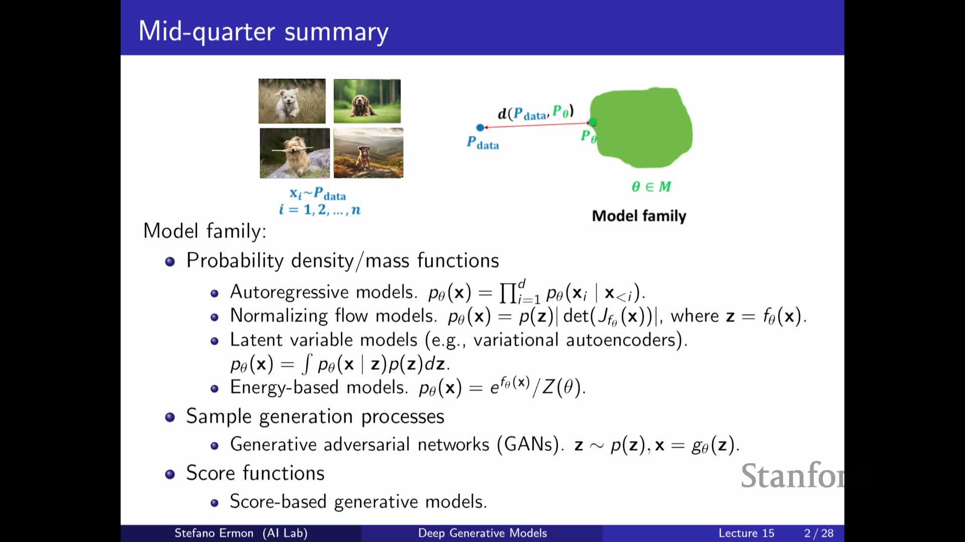
This segment introduces the lecture objective: to survey methods for evaluating generative models, and to emphasize that evaluation is a challenging open problem with no single consensus metric.
Evaluation is framed as essential for:
-
Comparing model families — e.g., autoregressive models, flows, latent-variable models, energy-based models (EBMs), GANs, and score-based models.
-
Guiding model and objective selection in both research and engineering contexts.
Motivations and connections:
- Evaluation helps decide which model is appropriate for a particular dataset and downstream use.
-
Quantitative assessment is critical for scientific progress and reproducibility in generative modeling.
Preview of evaluation goals:
- Different goals require different metrics, for example:
- Density estimation
- Sample quality / perceptual realism
-
Representation utility (for downstream tasks)
Evaluative comparison requires defining what ‘‘better’’ means for a task

This segment defines evaluation as the process of determining whether Model A is better than Model B, and it emphasizes that this comparison requires a clear notion of the task or objective.
Key points:
- Multiple model families and training objectives exist, so selection must be driven by the property that matters most for the intended use case:
- Density estimation
- Sampling quality
-
Representation learning
- Practical research motivation:
- Open-source models enable iterative improvements, which in turn require objective evaluation criteria to establish real progress.
- Open-source models enable iterative improvements, which in turn require objective evaluation criteria to establish real progress.
Setup for the lecture:
- Different evaluation metrics are appropriate depending on the end goal; the rest of the lecture explores which metrics align with which goals.
Evaluating generative models is harder than discriminative models because the task is ill-defined
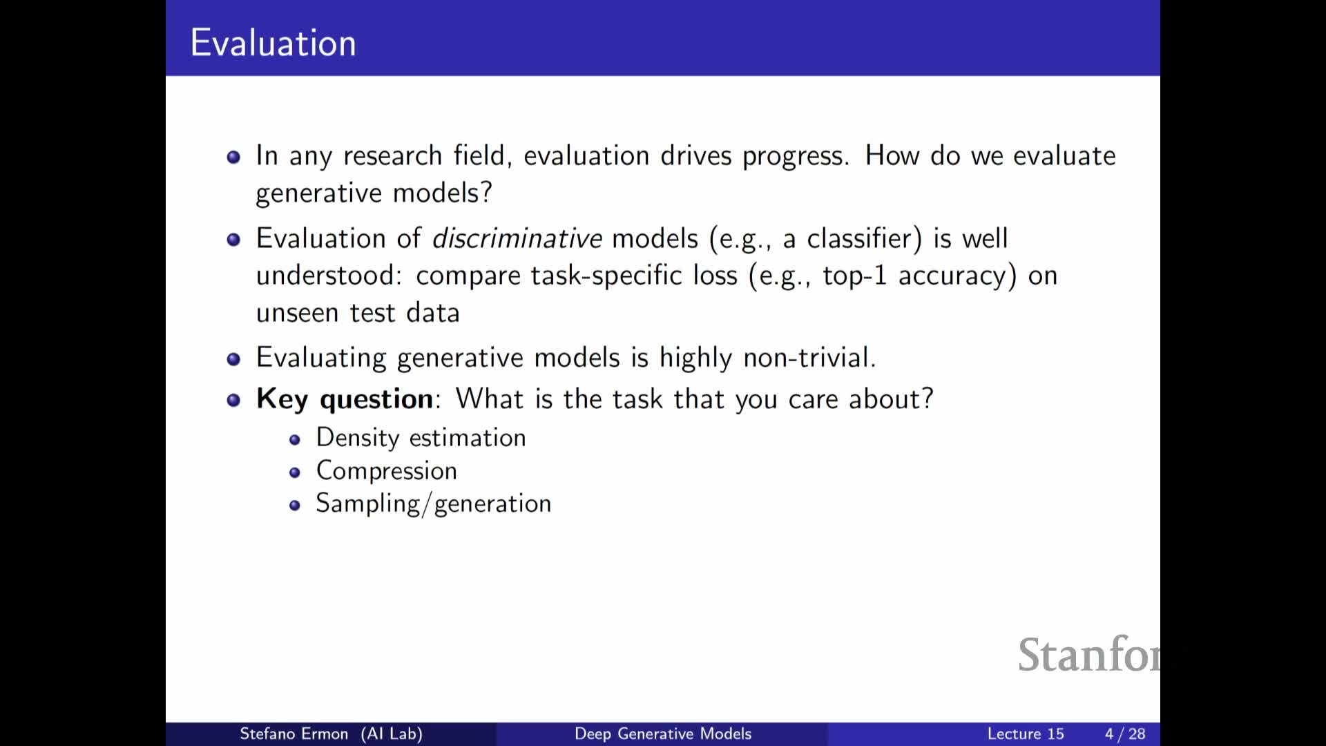
This segment contrasts evaluation for discriminative models with evaluation for generative models.
For discriminative models (e.g., classifiers):
- Tasks and metrics (like accuracy) are typically well defined.
- There is usually a clear loss function and a well-specified test distribution, enabling straightforward comparison on held-out data.
For generative models:
- The underlying task is often ambiguous because many objectives are possible:
- Likelihood
- Sampling fidelity / perceptual quality
- Compression
- Representation learning
-
Downstream task performance
Takeaway:
- Choosing an evaluation metric requires specifying the downstream or operational use of the generative model, since different metrics capture different aspects of performance.
Likelihood (average log-likelihood) is the canonical metric for density estimation and relates to compression
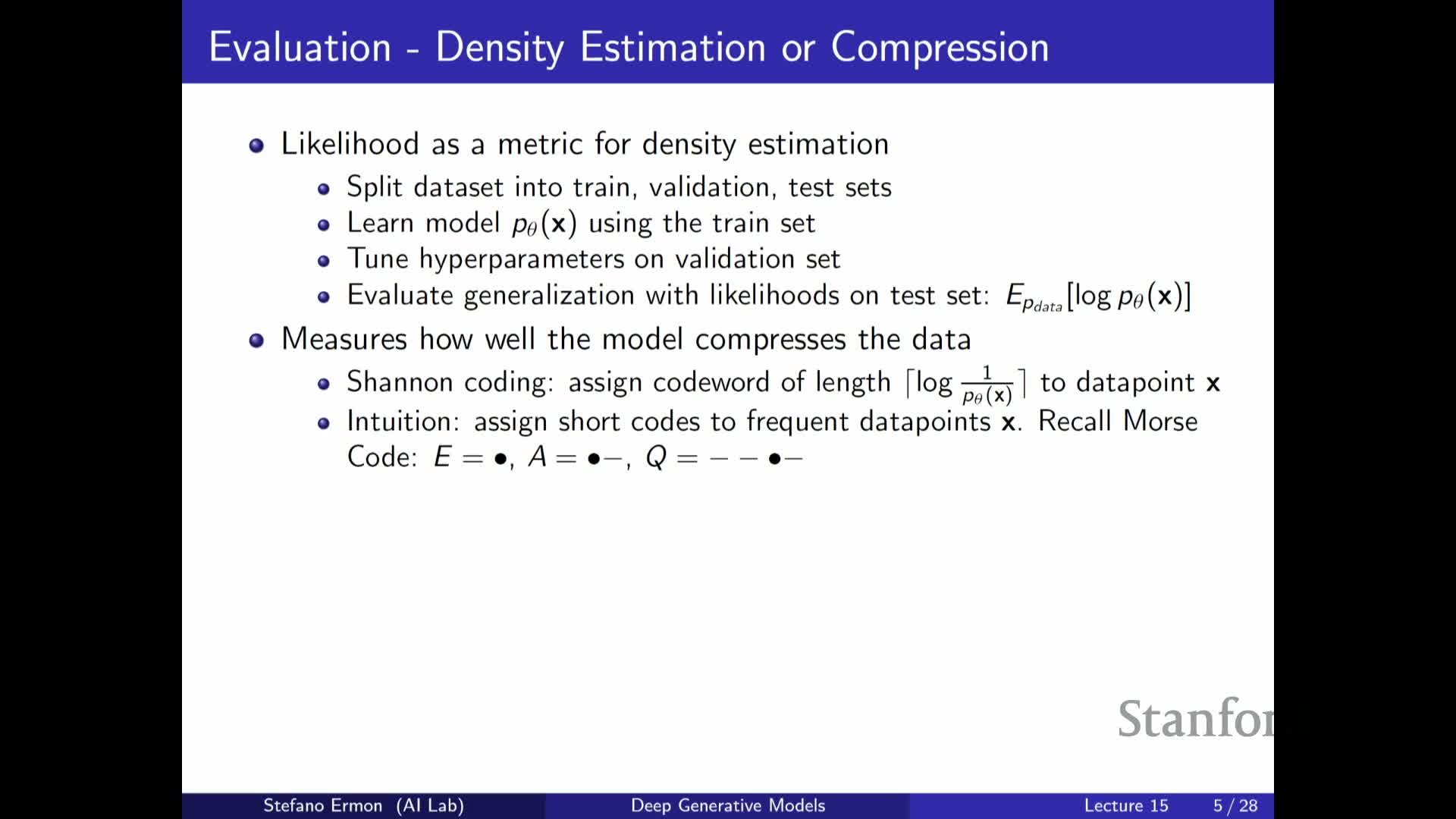
When the goal is accurate density estimation, average log-likelihood on held-out data (equivalently minimizing Kullback–Leibler divergence) is a principled metric.
Practical evaluation procedure:
-
Split the data into train / validation / test sets.
-
Select hyperparameters using validation data to avoid overfitting.
-
Report average log-likelihood on test data as the measure of model fit.
Connection to compression:
-
Maximum likelihood is directly tied to lossless compression under Shannon information theory: better likelihoods imply shorter expected code lengths.
- Practical schemes like arithmetic coding can approach the theoretical limits implied by likelihood estimates.
Compression objective captures structure but has limitations for downstream importance of bits

This segment argues why likelihood-based compression is useful and also highlights its limitations.
Why it helps:
- Compression forces models to identify redundancy and structure in data, which often corresponds to learning salient relationships.
- Historical motivations (e.g., the Hutter Prize) link compression to measures of intelligence and modeling skill.
- Empirical comparisons (e.g., human next-character prediction vs. modern language models’ bits-per-character) illustrate how compression quantifies learned regularities.
Crucial limitations:
-
Not all bits are equally important for downstream tasks — compression treats every bit the same.
- Compression treats all prediction errors equally, regardless of semantic impact (life-critical vs. cosmetic features).
- Therefore, likelihood alone may not prioritize task-relevant semantics, motivating alternative evaluation criteria when the goal is not pure density estimation.
Models without tractable likelihoods (GANs, EBMs) complicate likelihood-based evaluation
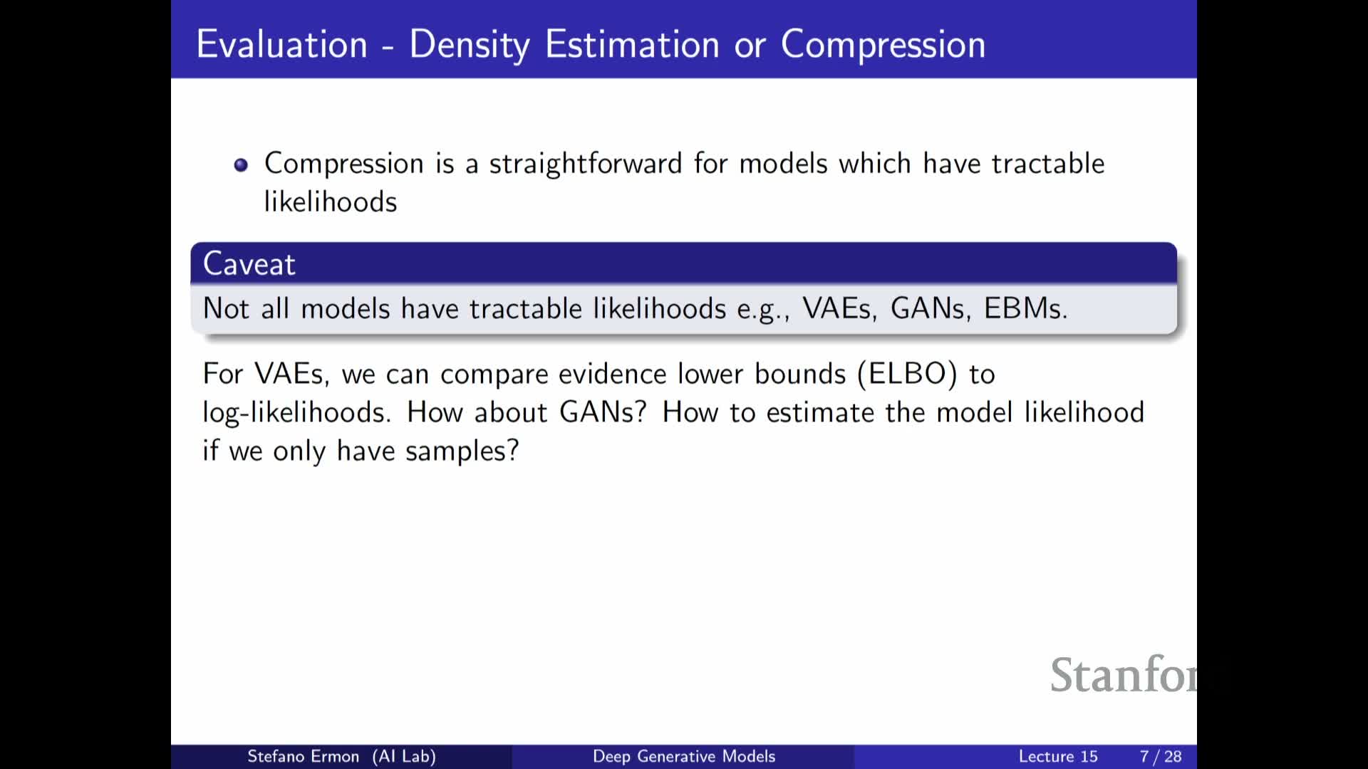
This segment explains a practical problem: many popular generative model classes do not provide tractable exact likelihoods, which complicates direct comparison via average log-likelihood or compression measures.
Relevant examples:
- GANs
- Some EBMs
- Certain VAEs, depending on tractability of the marginal likelihood
Practical notes:
- For VAEs, the ELBO provides a lower bound on log-likelihood, but translating ELBO differences into comparable likelihoods across model families is problematic.
- Practitioners therefore rely on alternative approximations or two-sample methods when exact likelihoods are unavailable.
-
Kernel density estimation and other sample-based density approximations are pragmatic options, but they have significant limitations (discussed next).
Kernel density estimation (KDE) approximates densities from samples via smoothing kernels but fails in high dimensions
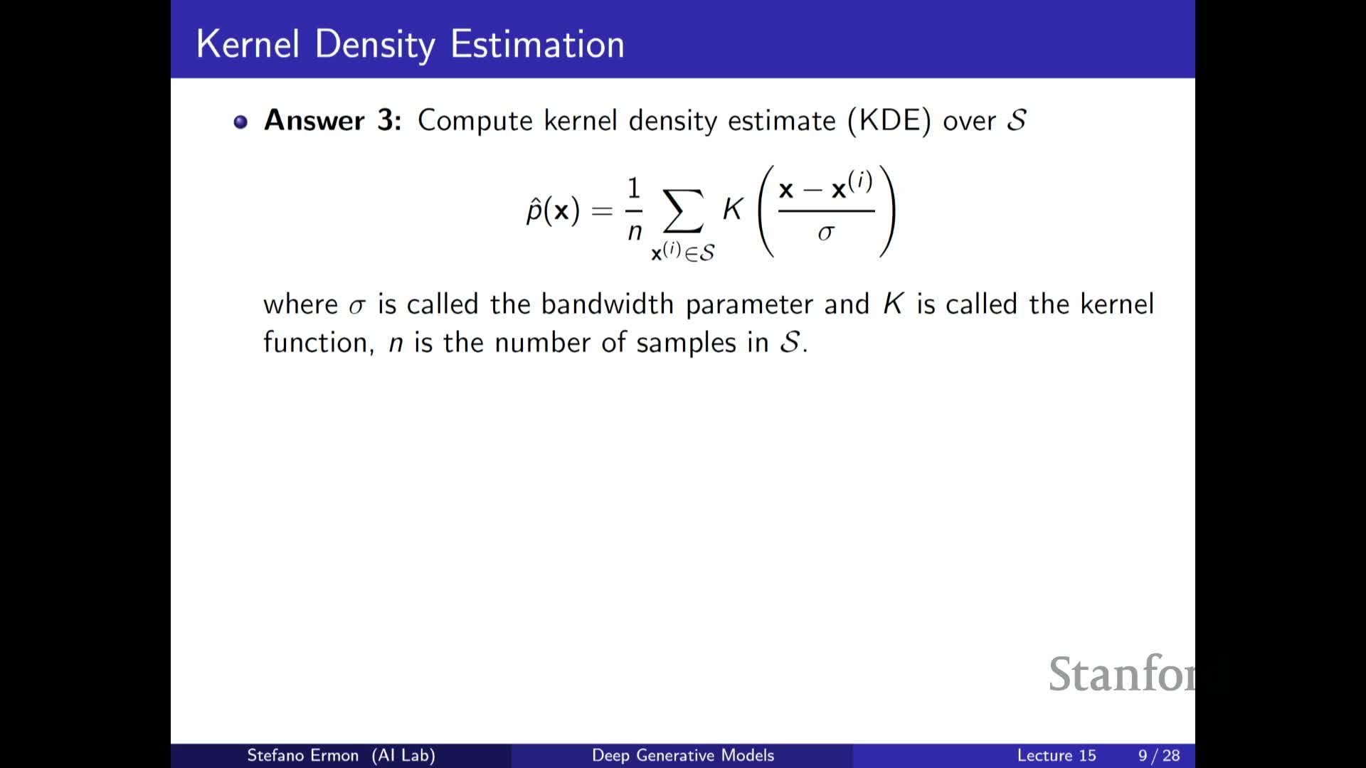
This segment describes histogram-based and kernel density estimators (KDEs) as sample-based approaches to approximate unknown model densities when only samples are available.
KDE mechanism (stepwise):
- Place a kernel (e.g., Gaussian) centered at each sample.
-
Sum the kernels across samples and divide by the sample count to obtain the density estimate.
- Control smoothness via the bandwidth parameter σ (larger σ = smoother estimate).
Practical aspects:
-
Kernel choice (Gaussian, Epanechnikov, etc.) matters but bandwidth selection is often more important.
-
Bandwidth selection is typically done by cross-validation to trade off bias and variance.
- There is a tension between undersmoothing (noisy estimate) and oversmoothing (loss of detail).
Major limitation:
-
Curse of dimensionality — KDE requires exponentially many samples as dimensionality grows (e.g., images), making KDE impractical for typical modern generative-modeling domains.
Estimating likelihoods for latent-variable models requires importance sampling and can have high variance
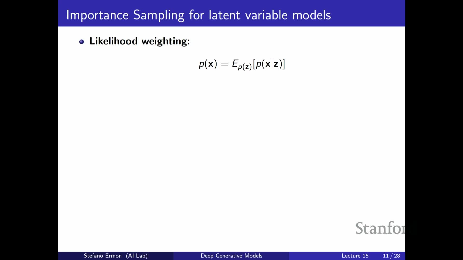
This segment treats latent-variable models and the challenge of estimating the marginal likelihood p(x) = ∫ p(x|z) p(z) dz.
Key points:
-
Naive Monte Carlo estimation (sampling z from the prior) can have high variance when the prior and posterior differ substantially.
-
Importance sampling can reduce variance by sampling from a proposal distribution closer to the posterior.
-
Annealed / bridged strategies (e.g., sequential importance sampling, annealed importance sampling) interpolate between the prior and posterior to obtain more accurate estimates.
Practical implications:
-
Naive sampling from the prior often yields poor likelihood estimates.
-
Specialized estimators can substantially improve accuracy when likelihood evaluation is required for model comparison in latent-variable settings.
Human evaluation remains the gold standard for sample quality but is costly and has caveats
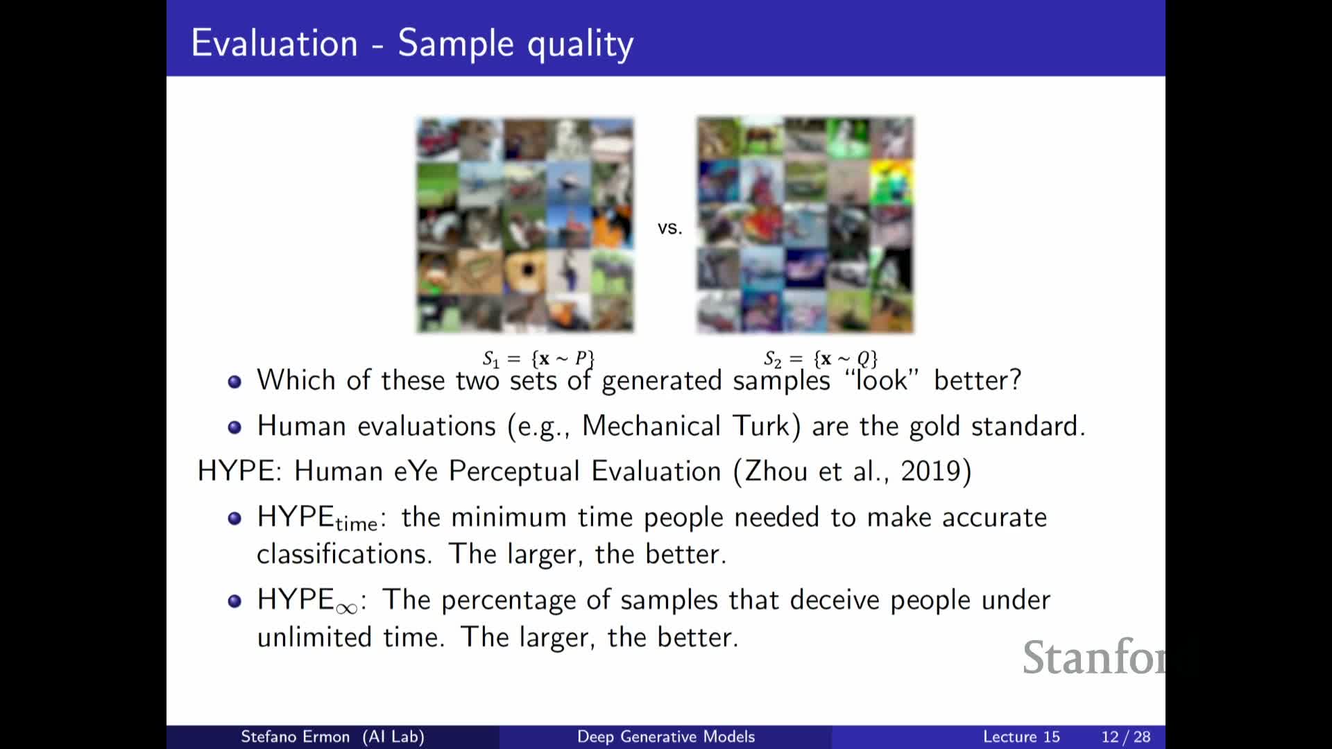
This segment advocates human perceptual studies as the most direct way to assess sample quality and visual realism.
Common protocols:
- Annotators compare real and generated samples or rate sample realism on a scale.
-
Psychological-style evaluations measure how long it takes humans to distinguish real from fake images — faster distinction implies lower sample quality.
- Measure deception rate when annotators have unlimited time (higher deception = higher perceptual realism).
Practical limitations:
- Human evaluations are expensive and difficult to scale during model development.
- Results are sensitive to task wording and experimental design, making reproducibility challenging.
- Human studies can fail to reveal memorization (a model that memorizes training images may still fool annotators but lacks generalization).
Inception Score measures sample sharpness and label diversity using a pretrained classifier
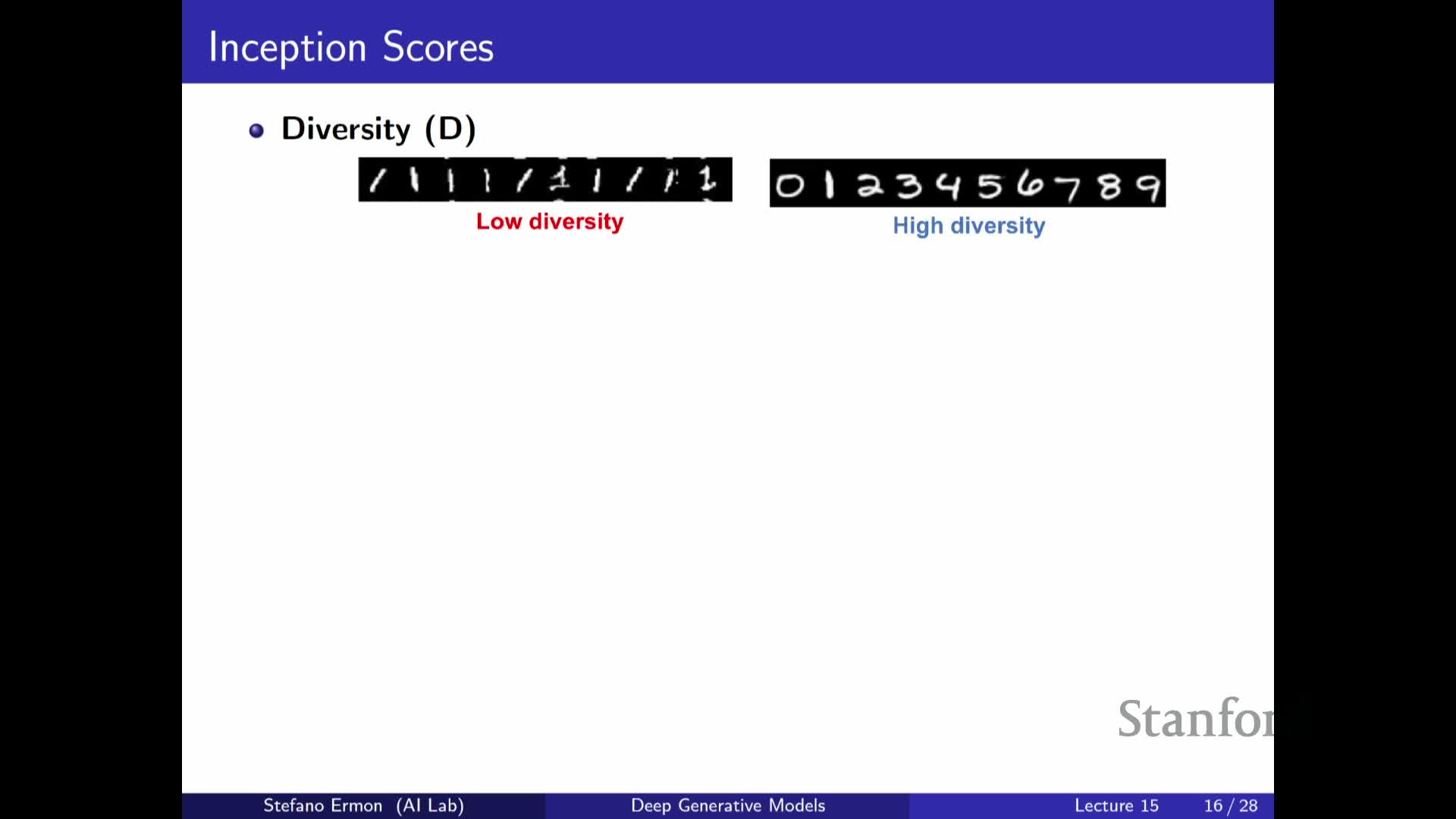
This segment defines the Inception Score (IS) as an automated metric for labeled image domains that leverages a pretrained classifier to assess two aspects of generated samples: sharpness and diversity.
How IS works (intuition):
-
Sharpness: low conditional entropy **p(y x)** indicates the classifier is confident about the class of a generated image.
-
Diversity: high entropy of the marginal p(y) across generated samples indicates coverage of many classes.
- The IS summarizes these by computing an exponentiated KL divergence between the conditional and marginal label distributions.
Limitations:
- IS inspects only generated samples, not how they compare to real data.
- It depends on the chosen classifier and label set, so results vary with the network used.
- IS can be gamed (e.g., produce images that maximize classifier confidence without capturing intra-class variability).
Fréchet Inception Distance (FID) compares pretrained feature distributions between real and generated data
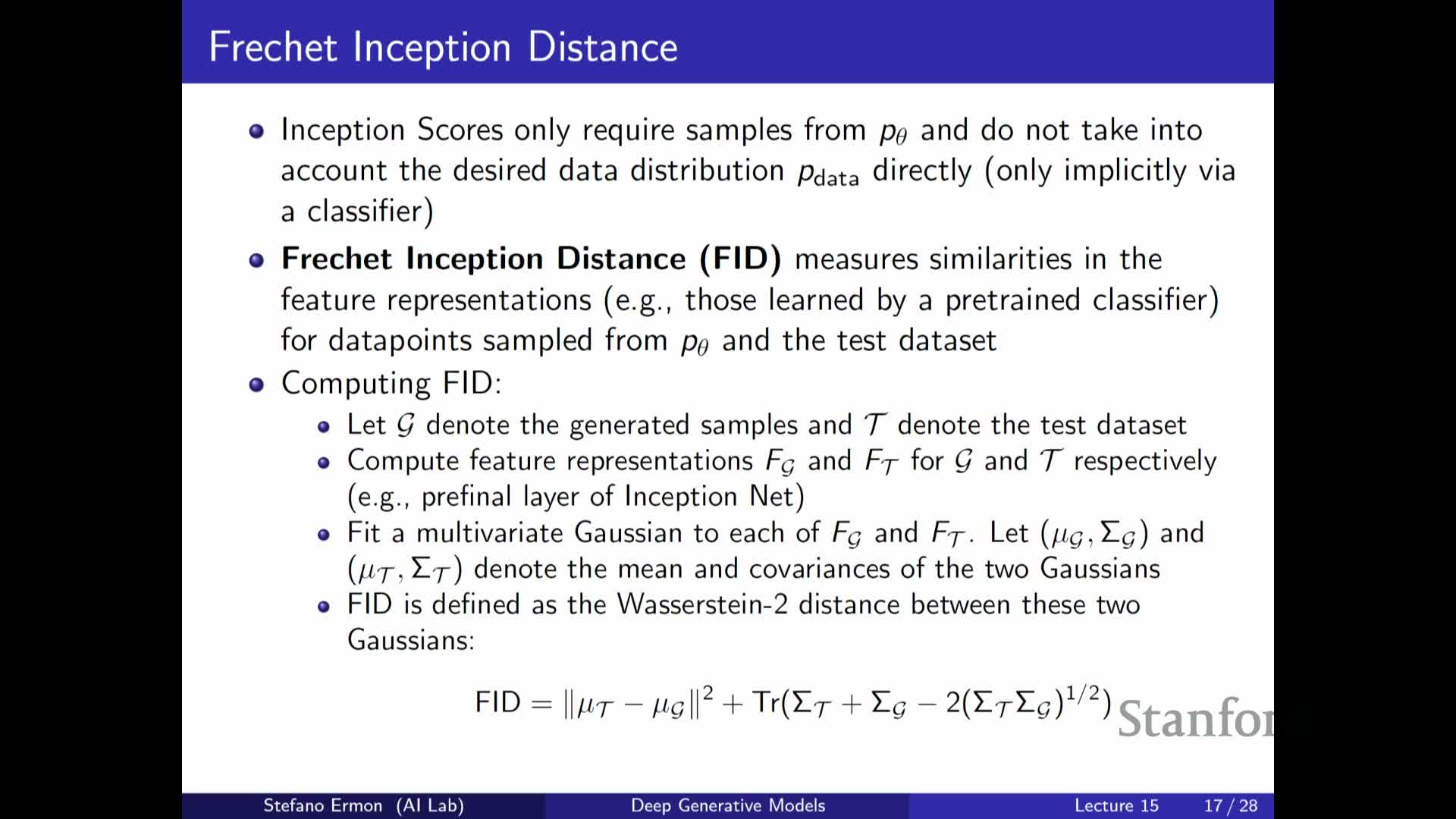
This segment describes the Fréchet Inception Distance (FID), a widely used metric that compares the distribution of pretrained-network features on real versus generated images.
Procedure:
- Compute activation vectors (e.g., Inception features) for many real and generated samples.
- Fit multivariate Gaussians to each feature set — estimate mean and covariance.
- Compute the Fréchet (Wasserstein-2) distance between these Gaussians; the distance has a closed-form expression in terms of means and covariances.
Intuition and trade-offs:
-
Smaller FID indicates generated features more closely match real data features, emphasizing higher-level perceptual features rather than raw pixels.
-
Kernel-based alternatives (e.g., MMD / KID) perform two-sample tests in feature space and can offer stronger statistical guarantees at higher computational cost.
Kernel-based two-sample tests (MMD/KID) operate in feature space and offer principled comparisons
This segment explains maximum mean discrepancy (MMD) and the kernel inception distance (KID) as kernel-based two-sample statistics.
Computation (intuition):
- Compare distributions by averaging pairwise kernel similarities:
- Average kernel value among real–real pairs
- Average among fake–fake pairs
- Average among real–fake pairs
- Combine these averages into a statistic that is zero iff the distributions match (for characteristic kernels).
Practical notes:
- Using pretrained-network features (e.g., Inception activations) as the kernel input emphasizes perceptual similarity rather than raw-pixel proximity.
- Trade-offs:
-
MMD/KID are more principled, but are computationally heavier (quadratic in sample count).
- They require careful kernel choice and scaling to be effective.
-
MMD/KID are more principled, but are computationally heavier (quadratic in sample count).
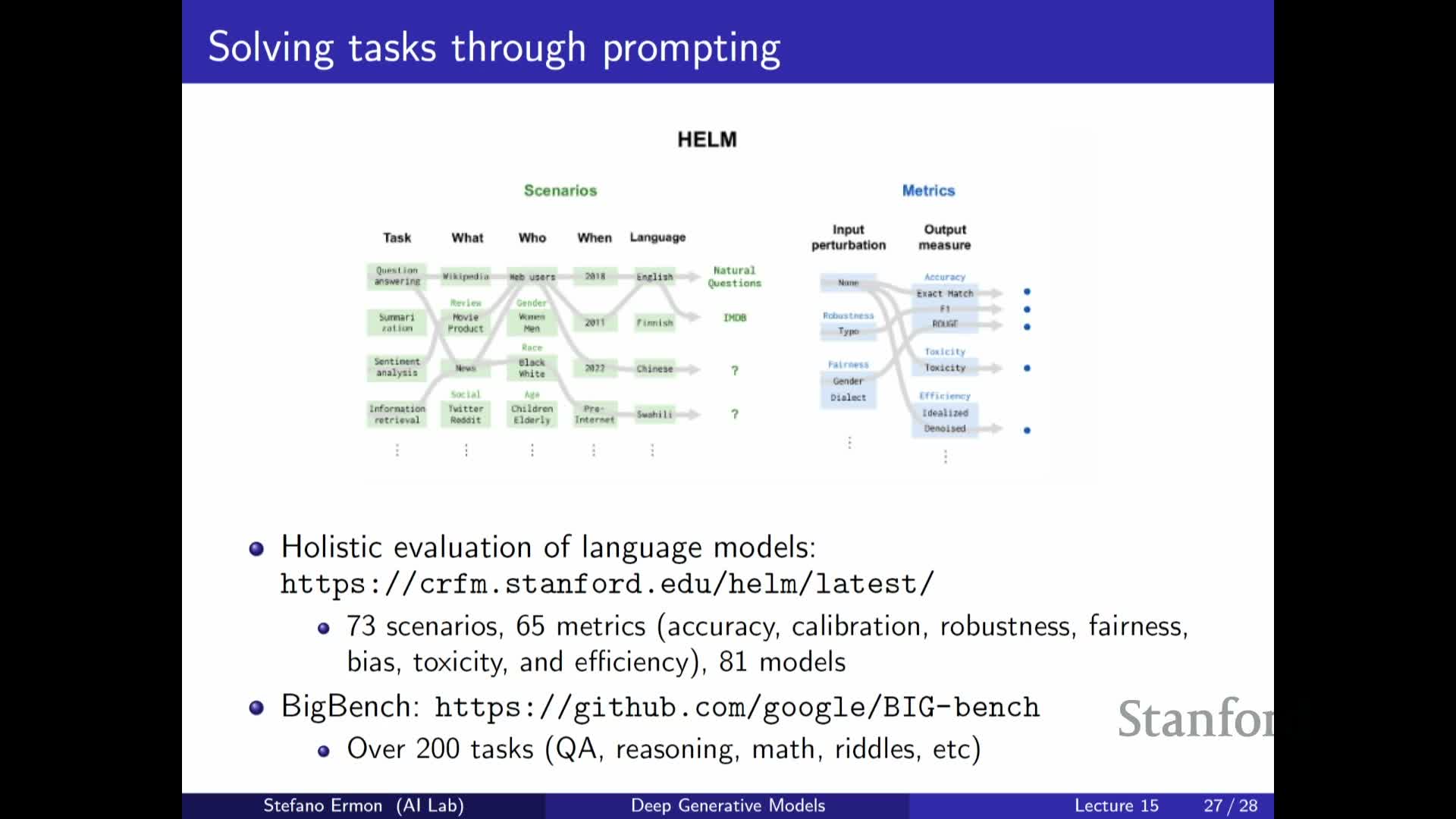
Holistic evaluation for conditional generative tasks (text-to-image) requires multiple specialized metrics
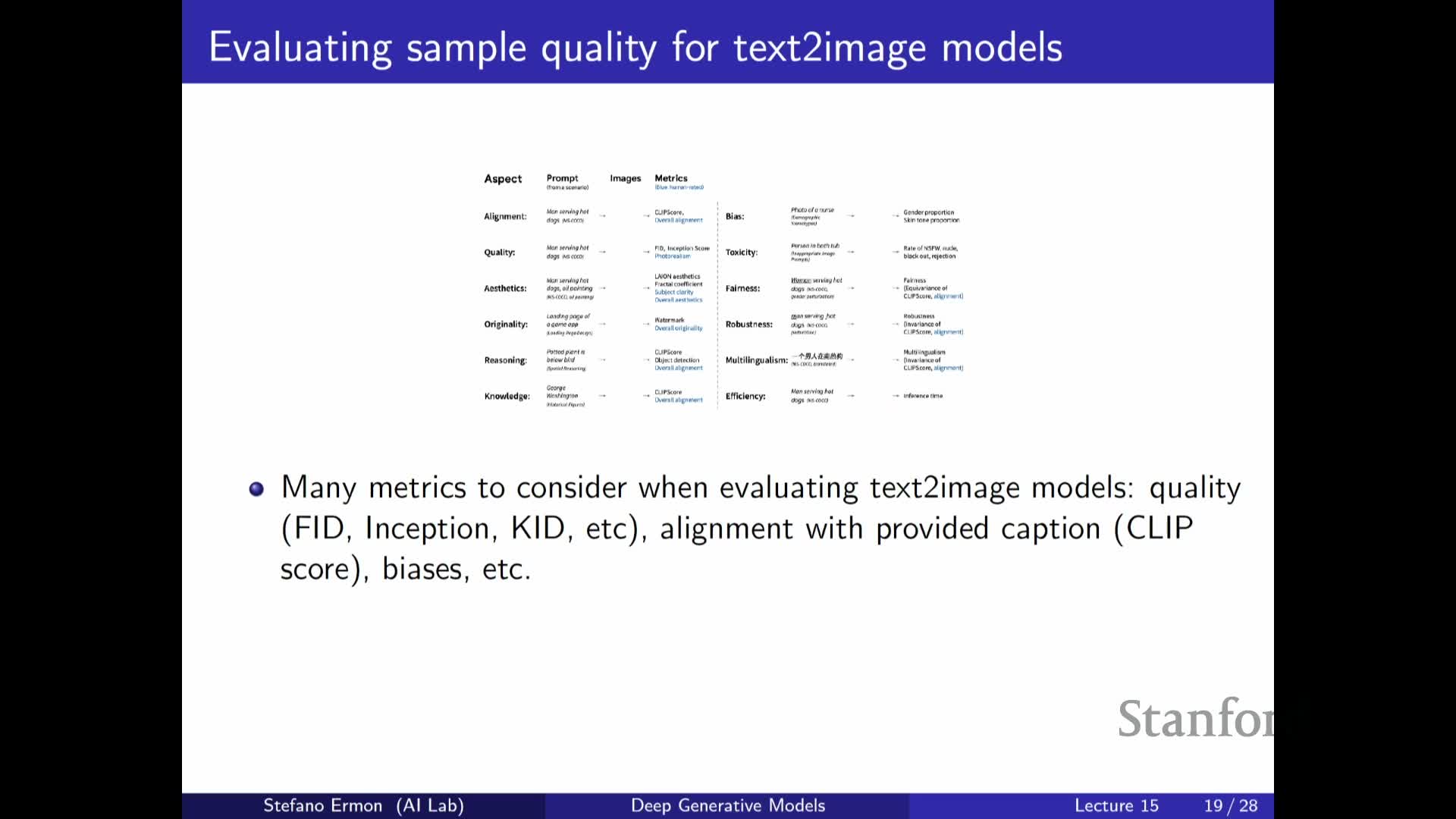
This segment observes that conditional generative tasks (e.g., text-to-image) require multifaceted evaluation beyond general sample quality because models must also respect the conditioning input and meet additional desiderata.
Recommended combined metrics:
-
Perceptual quality (e.g., FID / IS)
-
Caption–image alignment (automated metrics and human alignment checks)
-
Robustness to prompt variations
-
Originality and aesthetic measures
-
Bias / toxicity assessments and safety-related checks
Practice:
- Holistic benchmark efforts aggregate many automated metrics and human studies to enable comprehensive comparisons.
-
No single metric suffices for complex conditional tasks — evaluations must be multidimensional.
Representation quality is evaluated via downstream tasks such as clustering, reconstruction, and supervised transfer
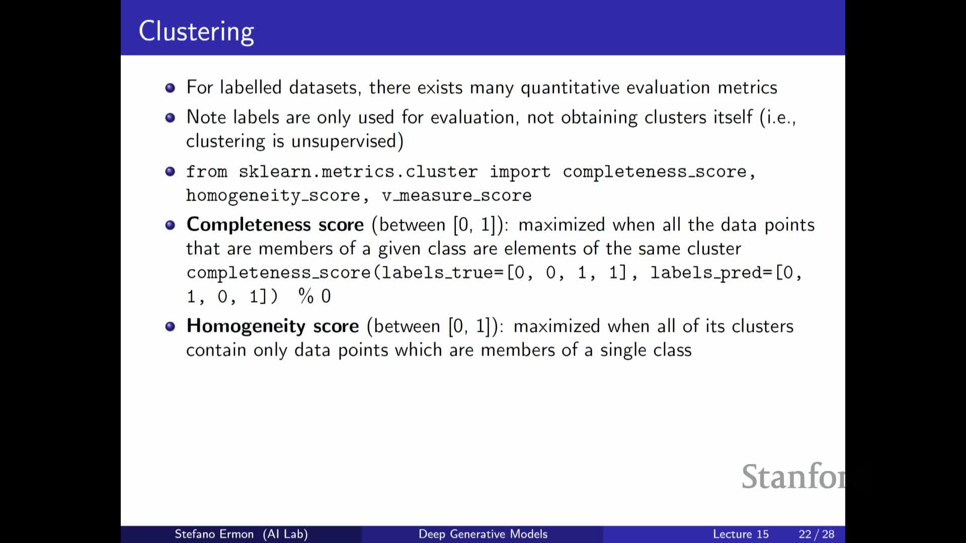
This segment discusses evaluating learned representations from generative models by measuring utility on downstream tasks.
Common evaluation paradigms:
- Map data to latent features, then:
- Apply simple classifiers to measure supervised performance (few-shot / linear-probe accuracy).
- Apply clustering (e.g., k-means) and report cluster-quality measures (completeness, homogeneity, V-measure).
- Apply simple classifiers to measure supervised performance (few-shot / linear-probe accuracy).
- Measure reconstruction fidelity for lossy-compression objectives using MSE / PSNR / SSIM.
- Quantify compression ratios (bits or dimensionality reduction) versus reconstruction quality.
Key point:
- The appropriate metric depends on the intended downstream use (classification, compression, clustering); representation comparisons are therefore necessarily task-dependent.
Disentanglement aims for interpretable latent factors but is provably unidentifiable without supervision

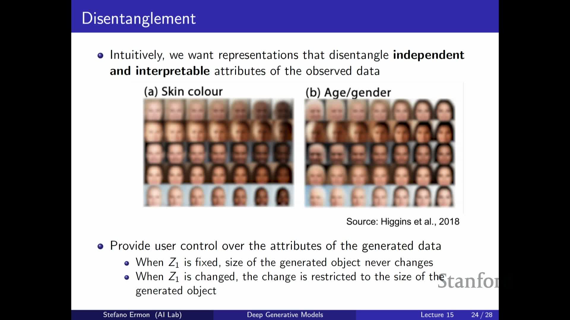
This segment defines disentanglement and explains theoretical and practical limitations.
Definition and measurement:
-
Disentanglement: latent variables correspond to independent, interpretable generative factors (e.g., pose, lighting, object identity).
- Practical metrics often use linear classifier accuracy to predict known factors from latent representations.
Theoretical limitation:
-
Fully unsupervised disentanglement is generally unidentifiable — without inductive biases or supervision, the mapping from data to factors is not unique, so provable recovery of true factors from unlabeled data alone is impossible.
Practical implication:
- Empirical methods sometimes produce disentangled representations, but success lacks general theoretical guarantees; reliable disentanglement typically requires supervision or structural constraints.
Pretrained language models can be adapted to downstream tasks via prompting or fine-tuning
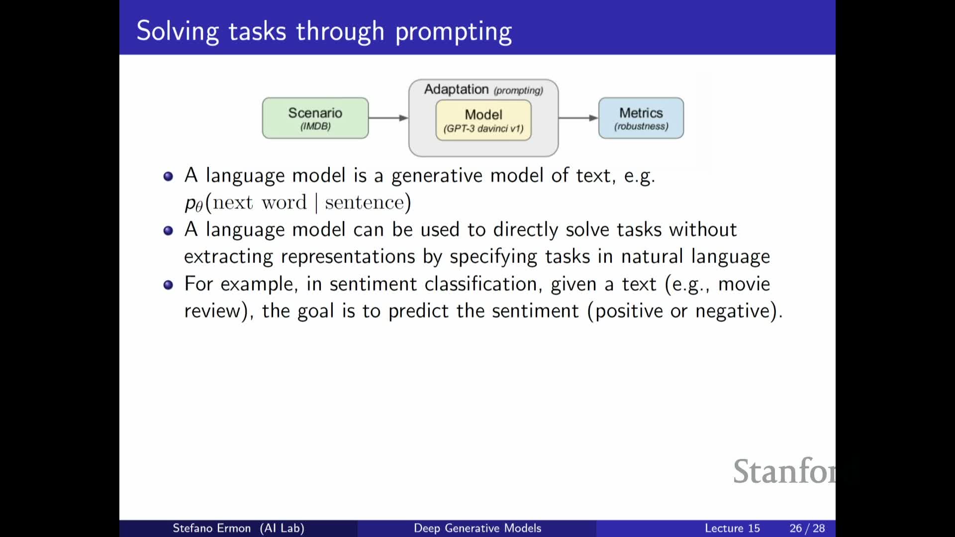
This segment explains how autoregressive language models trained by maximum likelihood can be adapted for downstream tasks via prompting or fine-tuning.
Two adaptation strategies:
-
Prompting:
- Craft a natural-language context that converts the task into next-token prediction (no parameter updates).
- Example pattern for sentiment classification: instruction + few examples + target (i.e., few-shot prompt).
- Advantages: requires no model updates and works with black-box API access.
- Craft a natural-language context that converts the task into next-token prediction (no parameter updates).
-
Fine-tuning:
- Modify model weights on labeled task examples to optimize task-specific performance.
- Advantages: usually yields higher task accuracy but requires compute and maintenance.
- Modify model weights on labeled task examples to optimize task-specific performance.
Operational trade-offs:
- Strong pretrained models often show useful few-shot / zero-shot behavior via prompting.
-
Fine-tuning typically improves accuracy at the cost of compute, storage, and operational complexity.
Prompting is less natural for non-sequential modalities but models can be adapted using preference data and fine-tuning
This segment considers extending the prompting paradigm beyond text and highlights challenges when model APIs emit images rather than discrete tokens.
Adaptation strategies for image or multimodal models:
- Collect preference or preference-pair data (which image is preferred for a caption).
- Fine-tune models to optimize for human preferences using preference learning or reinforcement learning from human feedback (RLHF) to improve aesthetics, reduce toxicity, or correct biases.
Research and trade-offs:
- Ongoing work aims to transfer instruction-style adaptation to vision and multimodal models.
- Practical trade-offs include the need for labeled preference data and the additional training effort required to implement preference-based fine-tuning.
Prompting versus fine-tuning: trade-offs in cost, accessibility, and performance

This segment compares prompting and fine-tuning as adaptation strategies for large pretrained models.
Summary of trade-offs:
-
Prompting
- Highly accessible: no retraining, works with black-box API access.
- Inexpensive in development time and easy to iterate.
- May provide strong few-shot/zero-shot capabilities, but typically limited compared to fine-tuning.
- Highly accessible: no retraining, works with black-box API access.
-
Fine-tuning
- Typically yields superior performance for many tasks.
- Requires compute resources, access to model weights or permissive APIs, and expertise in training.
- Better suited for repeated or large-scale deployments where higher accuracy justifies the cost.
- Typically yields superior performance for many tasks.
Recommendation:
- Select the strategy according to resource constraints, privacy requirements, desired performance, and deployment scale; both approaches are actively used depending on context.
Evaluation of generative models remains an open research area requiring multiple complementary metrics

This closing segment summarizes the core takeaways about evaluation in generative modeling.
Core messages:
-
Evaluation is an open problem with many partial solutions; there is no one-size-fits-all metric.
- Metrics must be chosen to reflect the downstream objective:
-
Likelihood for density estimation
-
Human / perceptual metrics for sample quality
-
Task-driven metrics for representation utility
-
Likelihood for density estimation
-
Large-scale benchmarks that aggregate diverse tasks and metrics are useful, but they do not resolve how to weight or prioritize different metrics.
Practical recommendations:
- Use a mixture of human and automated evaluations.
- Practice careful experimental design to ensure reproducibility.
- Continue research into new evaluation methodologies tailored to specific generative modeling applications.
Enjoy Reading This Article?
Here are some more articles you might like to read next: