Stanford CS236- Deep Generative Models I 2023 I Lecture 16 - Score Based Diffusion Models
- Lecture overview and goals
- Score-based models represent densities via their score function and are trained by denoising score matching on perturbed data
- The forward diffusion defines a fixed Markov encoder that maps data to a sequence of increasingly noisy latent variables by adding Gaussian noise incrementally
- Repeated Gaussian perturbations produce analytically tractable marginals and give the forward process a diffusion (heat) interpretation
- The reverse generative process is approximated by parameterizing reverse conditionals as Gaussians with neural-network predicted parameters
- Maximizing the diffusion ELBO with a particular mean parameterization is equivalent to denoising score matching, which yields the DDPM training objective
- Practical model design hinges on choices for the fixed encoder, noise schedule, loss weighting, and neural architecture
- The infinitesimal limit of the discrete diffusion yields a continuous-time SDE whose time-reversal depends on the score function and is solved numerically for sampling
- The diffusion SDE admits an equivalent deterministic probability-flow ODE with identical time-marginals, enabling invertible flow formulations and exact likelihood computation
Lecture overview and goals
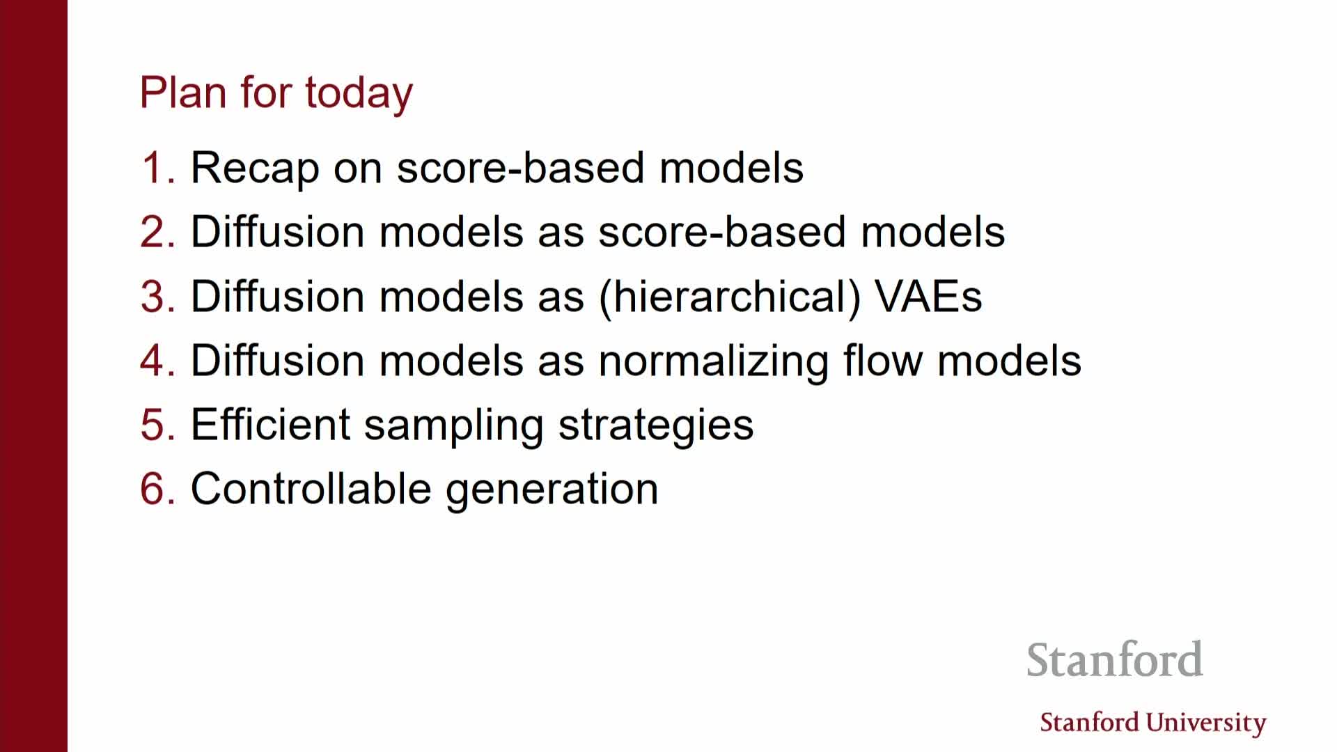
This lecture ties together several foundational ideas in modern generative modeling: score matching, diffusion models, variational autoencoders, SDE/ODE interpretations, and practical sampling and control techniques.
- It explains how score-based models can be viewed both as diffusion processes and as hierarchical variational autoencoders.
- It shows that the reverse process of a diffusion yields flows with exact likelihoods when expressed as a probability-flow ODE.
- It outlines how numerical solvers and conditioning enable efficient, controllable generation in practice.
- The talk previews formal comparisons between denoising score matching objectives and the evidence lower bound (ELBO), and highlights practical topics such as sampling acceleration and conditioning for tasks like text-to-image generation.
This high-level overview frames the technical developments and motivates the equivalences and algorithms developed later in the lecture.
Score-based models represent densities via their score function and are trained by denoising score matching on perturbed data
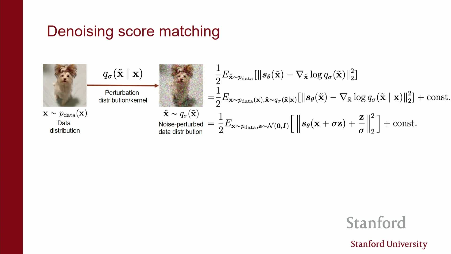
Score function: the gradient of the log density with respect to inputs — it defines a vector field that points toward higher-probability regions.
- Neural networks are used to approximate this vector field, but direct score matching is computationally challenging in high dimensions.
-
Denoising score matching solves this by training a network to predict the score of a noise-perturbed version of the data — equivalently, to learn to remove Gaussian noise from noisy inputs.
- Training reduces to a regression-like objective where the network predicts either the added noise or the denoised signal.
-
Amortization across multiple noise levels is achieved by conditioning the network on the noise intensity (e.g., a time or sigma input).
- Training reduces to a regression-like objective where the network predicts either the added noise or the denoised signal.
- Sampling from the learned score field uses stochastic-gradient dynamics such as Langevin dynamics.
- Initialize from noise.
- Run iterative score-guided updates (and possibly injected noise) to move samples toward higher-density regions.
- Initialize from noise.
- Practical methods use a sequence of noise levels — annealed or multi-scale — to progressively refine samples from pure noise toward the data manifold.
Trade-off: the model learns scores of noisy distributions rather than the clean data distribution. This is more scalable, but it changes the exact target of estimation (the network models s(x; sigma) for noisy marginals rather than s(x; 0)).
The forward diffusion defines a fixed Markov encoder that maps data to a sequence of increasingly noisy latent variables by adding Gaussian noise incrementally
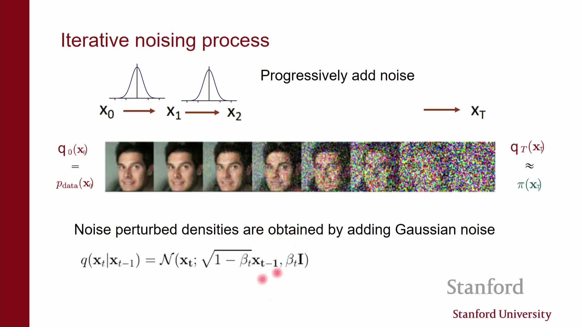
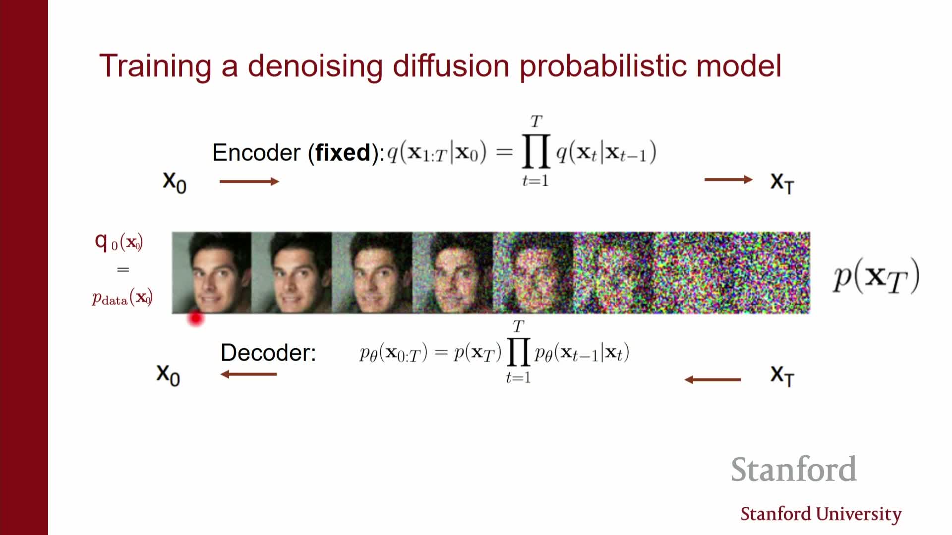
Forward / encoder process: a simple, fixed Markov chain Q that maps x0 → x1 → … → xT by repeatedly adding Gaussian noise (optionally with rescaling).
-
Each conditional Q(xt xt-1) is a Gaussian with known mean and variance, so the full joint factorizes as a product of simple conditionals.
-
Because repeated Gaussian kernels compose analytically, any marginal Q(xt x0) is itself a closed-form Gaussian — this makes simulation and marginal sampling efficient.
- Important design points:
- The encoder Q is not learned; it is a deterministic design choice that defines multiple noisy views of each data point.
- The latent representation is the entire trajectory x1:T, which is higher-dimensional than x0 and generally not invertible because noise is added at every step.
- This structured latent family is well suited to variational approximations, and it underpins treating diffusion models as hierarchical variational autoencoders with a fixed encoder.
- The encoder Q is not learned; it is a deterministic design choice that defines multiple noisy views of each data point.
Repeated Gaussian perturbations produce analytically tractable marginals and give the forward process a diffusion (heat) interpretation
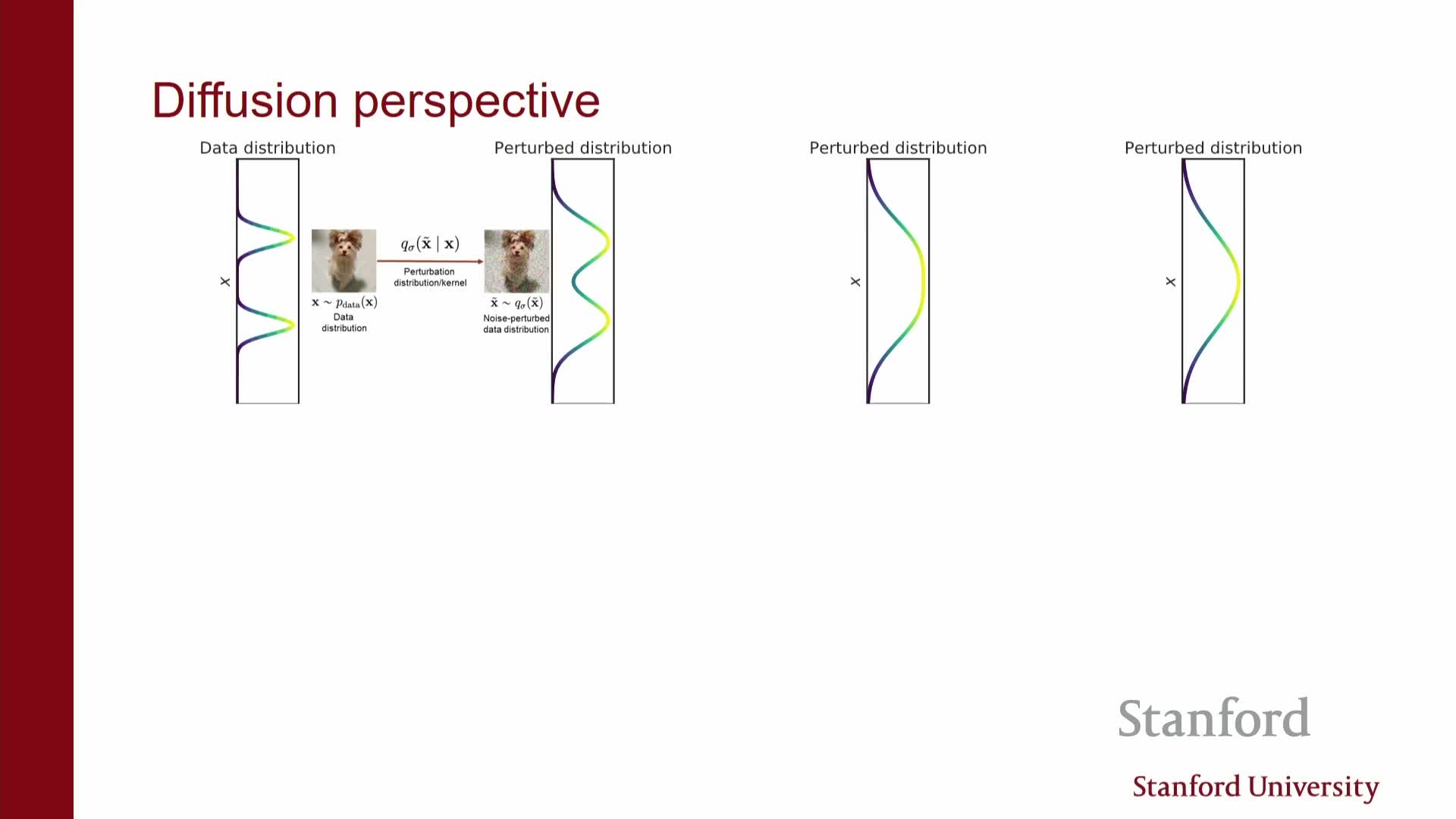
When Gaussian noise is applied incrementally, composing the stepwise kernels yields another Gaussian whose mean and variance can be computed in closed form by composing the step parameters.
- As a consequence, one can directly sample any marginal Q(xt) without simulating the entire chain from x0.
- Interpreting the incremental noising as a diffusion process gives an intuition: probability mass spreads out like heat. This continuous viewpoint motivates choosing kernels that destroy structure gradually, so the terminal distribution becomes simple and easy to sample from.
- Two practical requirements arise from this interpretation:
- The forward process must reliably erase structure so the end state is a known simple prior.
- The intermediate marginals must be efficiently sampleable, because they supply training examples for denoising score matching.
- The forward process must reliably erase structure so the end state is a known simple prior.
- These considerations justify the widespread use of Gaussian transition kernels and carefully designed noise schedules in diffusion models.
The reverse generative process is approximated by parameterizing reverse conditionals as Gaussians with neural-network predicted parameters
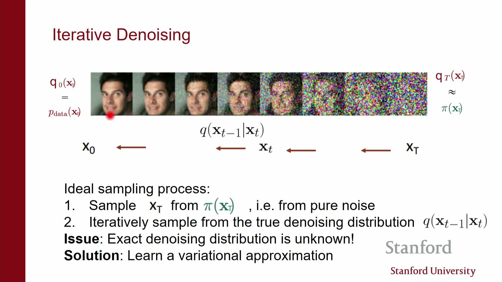
The true reverse kernel Q(xt-1 | xt) is generally unknown, so the learned decoder P_theta approximates it with Gaussian conditionals P_theta(xt-1 | xt) whose means (and sometimes variances) are produced by neural networks.
Sampling from the generative model proceeds as follows:
- Sample xT from a simple prior (e.g., standard Gaussian that the forward process converges to).
-
For t = T, …, 1: sample xt-1 from P_theta(xt-1 xt).
- Output x0 as the generated sample.
- This mirrors the variational decoder in a hierarchical VAE: the fixed forward chain Q is the encoder and P_theta is the learned decoder.
- Parameters theta are chosen to make the approximate reverse conditionals close to the true reverse conditionals (typically by minimizing KL divergence terms in the ELBO).
- Proper selection of stepwise noise parameters (betas/alphas) ensures the forward chain actually converges to the simple prior and makes the variational approximation tractable to learn.
Maximizing the diffusion ELBO with a particular mean parameterization is equivalent to denoising score matching, which yields the DDPM training objective
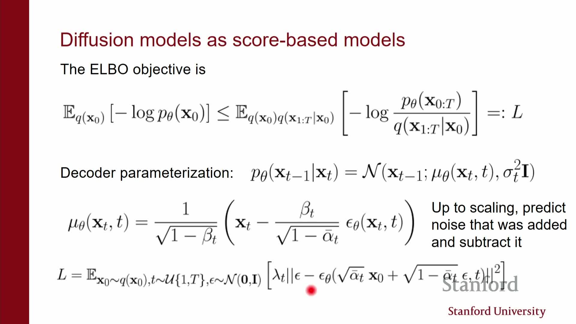
Evidence lower bound (ELBO) for the diffusion VAE compares the fixed forward chain Q(x1:T | x0) to the learned reverse chain P_theta(x0:T) and simplifies to tractable terms because Q is Gaussian and fixed.
- If the decoder means are parameterized via an epsilon network that predicts the noise added to xt (so the mean is xt minus a scaled estimate of that noise), the ELBO terms algebraically simplify and become equivalent to a denoising score matching objective that trains the network to predict the added noise.
- This explains why the DDPM training procedure, which directly trains a noise-predicting network, matches a principled variational objective.
- This explains why the DDPM training procedure, which directly trains a noise-predicting network, matches a principled variational objective.
- Sampling options after training:
-
Ancestral sampling from the learned decoder Gaussians (the DDPM procedure).
-
Langevin-style iterative refinement using the learned score model.
-
Ancestral sampling from the learned decoder Gaussians (the DDPM procedure).
- Both approaches take the form of gradient-plus-noise steps, but they differ in discretization and scaling, which leads to different empirical behavior and trade-offs.
Practical model design hinges on choices for the fixed encoder, noise schedule, loss weighting, and neural architecture
Fixing the forward encoder to incremental Gaussian noising simplifies training and often yields better sample quality than attempting to jointly learn a flexible encoder.
- Trade-offs of learning the encoder vs keeping it fixed:
- Fixed encoder: simpler optimization, often better sample fidelity.
- Learned encoder: can improve the ELBO but may reduce sample fidelity and increase optimization complexity.
- Fixed encoder: simpler optimization, often better sample fidelity.
-
Loss weighting factors (lambda_t) control emphasis on different noise levels in the ELBO.
- In practice, practitioners often use uniform or scaled weights rather than the exact ELBO-prescribed weights — this alters likelihood optimization behavior and can improve perceptual sample quality.
- In practice, practitioners often use uniform or scaled weights rather than the exact ELBO-prescribed weights — this alters likelihood optimization behavior and can improve perceptual sample quality.
-
Beta schedule (and derived alphas) controls how quickly structure is destroyed. It can be tuned or learned to trade off training stability, sample quality, and compute cost; many empirical studies focus on finding schedules that give good generative performance.
- Architectural choices:
-
U-Net–like image-to-image networks are the dominant practical choice for the epsilon or score network because they provide strong inductive biases for dense prediction.
-
Transformers and other architectures can also be applied, but they typically require careful engineering to match U-Net performance in this domain.
-
U-Net–like image-to-image networks are the dominant practical choice for the epsilon or score network because they provide strong inductive biases for dense prediction.
The infinitesimal limit of the discrete diffusion yields a continuous-time SDE whose time-reversal depends on the score function and is solved numerically for sampling

As the discretization is refined, the forward Markov chain converges to a stochastic differential equation (SDE) that describes x_t with a deterministic drift and an infinitesimal diffusion term — this forward SDE corresponds to the encoder diffusion.
- The exact reverse-time process that maps noise back to data is another SDE whose drift depends explicitly on the time-dependent score function of the forward marginal at time t. Therefore, an accurate time-dependent score model s_theta(x, t) is sufficient to characterize the exact reverse dynamics.
- In practice:
- The learned score network evaluates s_theta(x, t).
- Numerical SDE solvers discretize the reverse SDE to generate samples.
- Different solver families — predictor, corrector, or predictor–corrector — correspond to different sampling algorithms and discretization strategies.
- The learned score network evaluates s_theta(x, t).
- Score-based sampling methods often interleave deterministic score-driven updates with localized MCMC or Langevin corrections to control numerical error; DDPM corresponds to a specific Euler–Maruyama discretization, while score-based frameworks can use more sophisticated integrators for improved trade-offs.
The diffusion SDE admits an equivalent deterministic probability-flow ODE with identical time-marginals, enabling invertible flow formulations and exact likelihood computation
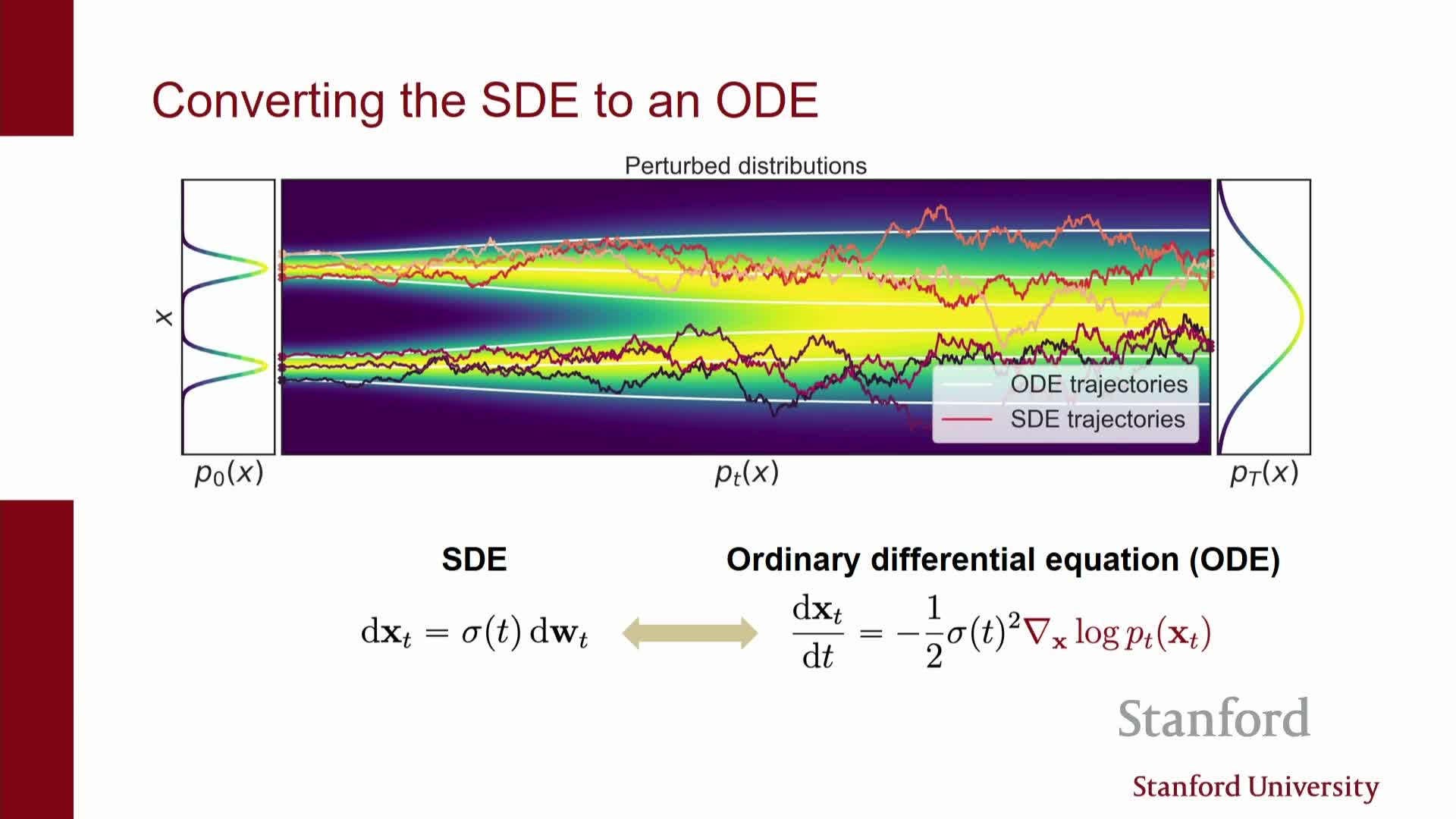
There exists a probability-flow ordinary differential equation (ODE) whose solution paths are deterministic and whose marginals at each time match those of the original SDE; the ODE drift can be expressed in terms of the score function and known SDE coefficients.
- Because the ODE mapping from xT to x0 is deterministic (and typically invertible), it defines a continuous normalizing flow and therefore permits exact likelihood evaluation via the change-of-variables formula by integrating the instantaneous Jacobian trace along the ODE trajectory.
- Converting a diffusion model to this deterministic flow requires the same time-dependent score estimates used for the reverse SDE, so both likelihoods and efficient deterministic sampling depend critically on score accuracy.
- The ODE perspective offers two principal advantages:
- Deterministic, potentially faster sampling using advanced ODE solvers.
- Access to exact likelihoods for evaluation, likelihood-based training, or model comparison.
- Deterministic, potentially faster sampling using advanced ODE solvers.
Enjoy Reading This Article?
Here are some more articles you might like to read next: