Stanford CS236- Deep Generative Models I 2023 I Lecture 17 - Discrete Latent Variable Models
- Lecture overview and plan
- Score-based models and DDPMs are equivalent perspectives on noising/denoising generative modeling
- ELBO training reduces to learning a sequence of denoisers and score functions
- Continuous-time diffusion (the diffusion limit) generalizes discrete-step DDPMs
- The forward process is an SDE with drift and diffusion describing noise addition
- Reverse-time SDE introduces a score-dependent drift used for sampling
- Score estimation and discretization yield DDPM-like denoising updates
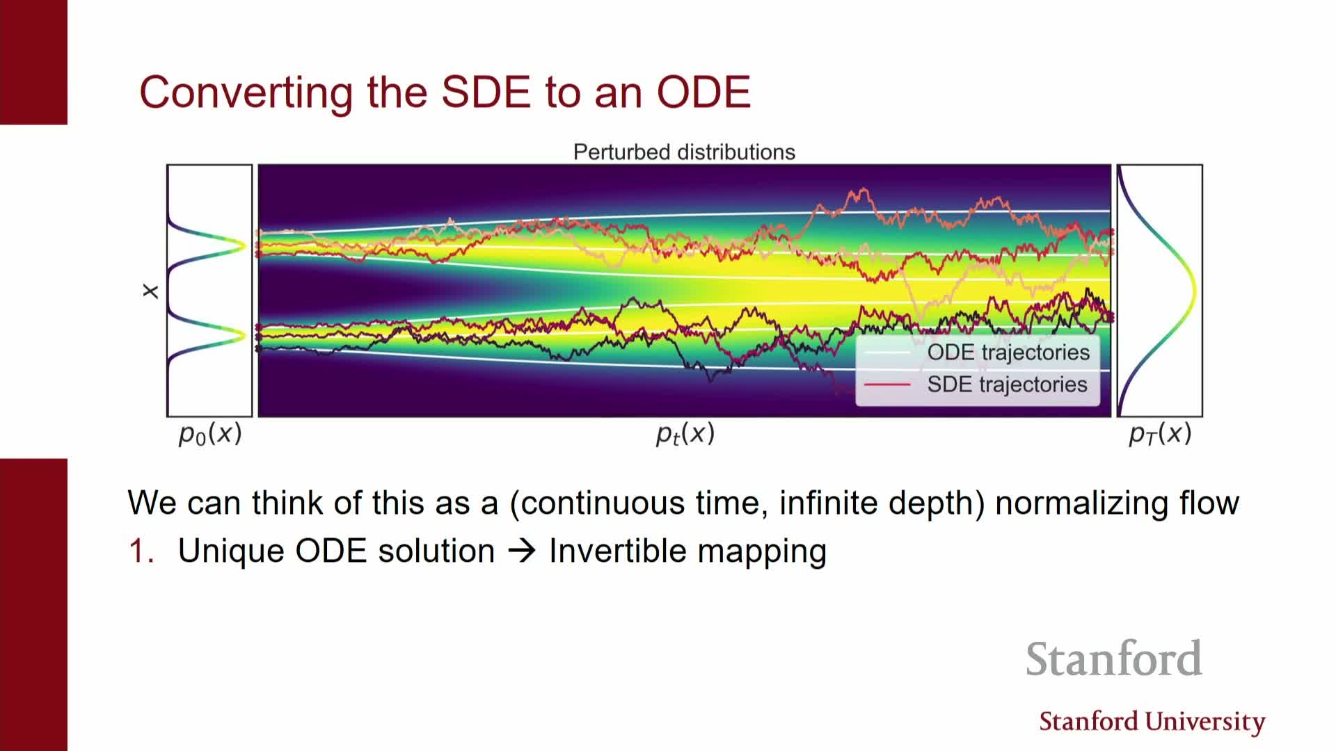
- An equivalent deterministic ODE (flow) exists with identical marginals
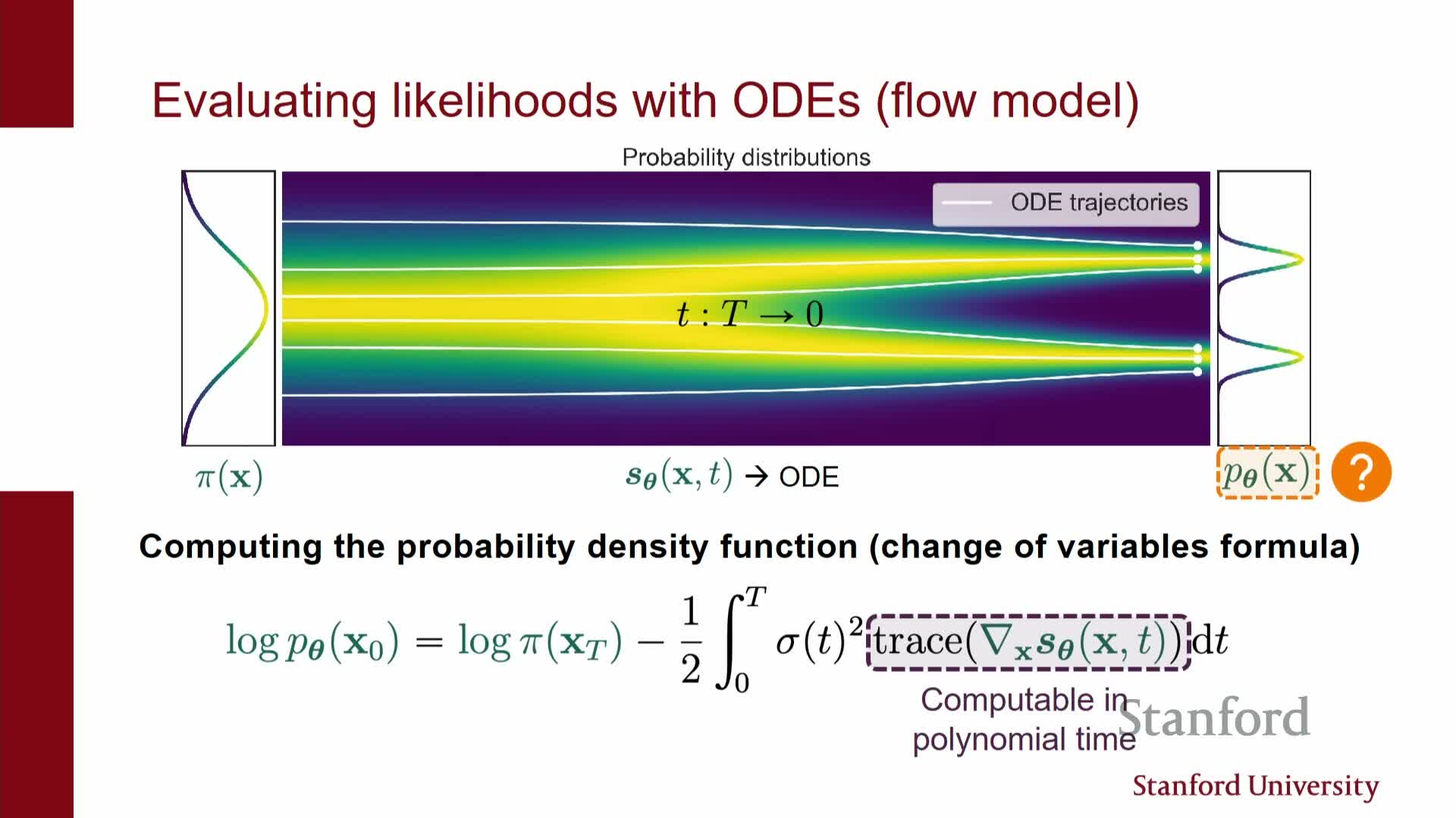
- Likelihood evaluation via ODE change-of-variables uses trace-Jacobian integration
- Sampling tradeoffs: ODEs give faster deterministic samples while SDEs provide robustness
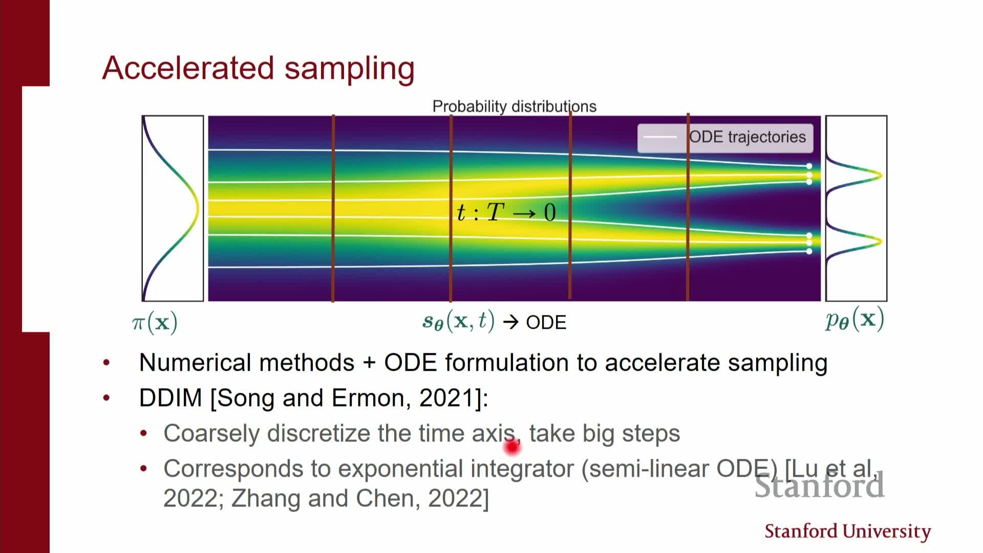
- Accelerated sampling methods (DDIM and coarse discretization) reduce step count
- Parallel-in-time ODE solvers trade compute for wall-clock speed by denoising trajectory segments concurrently
- Progressive distillation and consistency models compress multi-step samplers into very few steps
- Latent diffusion uses a VAE-style encoder to reduce dimensionality and accelerate training and sampling
- Conditional generation is implemented by supplying side information to the score/denoiser network
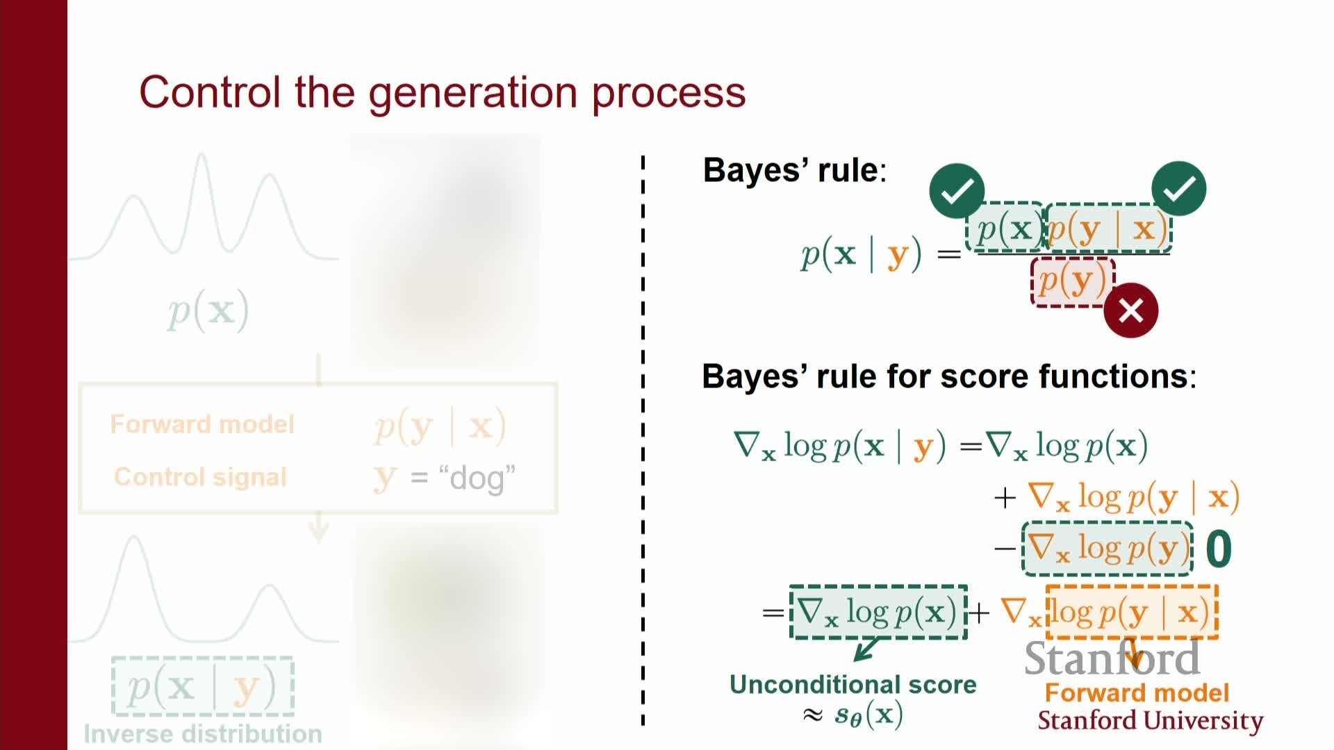
- Bayesian conditioning via classifier guidance: posterior scores equal prior plus likelihood score
- Classifier guidance and classifier-free guidance provide practical conditioning mechanisms
- Applications include image editing, inverse problems, and medical imaging where likelihoods encode measurement physics
- Classifier-free guidance and other practical tricks avoid explicit classifier training
- Recent engineering advances yield real-time or very low-step generation by combining distillation, latent models, and advanced solvers
- Summary: score estimation unlocks multiple inference paradigms and practical tradeoffs
Lecture overview and plan
This segment outlines the lecture’s objective to continue the exploration of diffusion models and to connect them with stochastic differential equations (SDEs) and ODE-based samplers.
It frames score-based models and denoising diffusion probabilistic models (DDPMs) as two perspectives on the same noising/denoising family of generative models and motivates moving from discrete-time VAEs to continuous-time formulations.
Practical interests emphasized in the lecture:
- Efficient samplers (fewer model evaluations, accelerated integrators)
- Exact and approximate likelihood evaluation (continuous-time change-of-variables)
- Conditional generation techniques (text-to-image, classifier-guided sampling)
The stage is set for formal descriptions of:
- Forward noising processes (how data is corrupted over time)
- Reverse-time dynamics (how to undo corruption using scores/denoisers)
-
Algorithmic implications for sampling and training (discretizations, solvers, and trade-offs)
Score-based models and DDPMs are equivalent perspectives on noising/denoising generative modeling
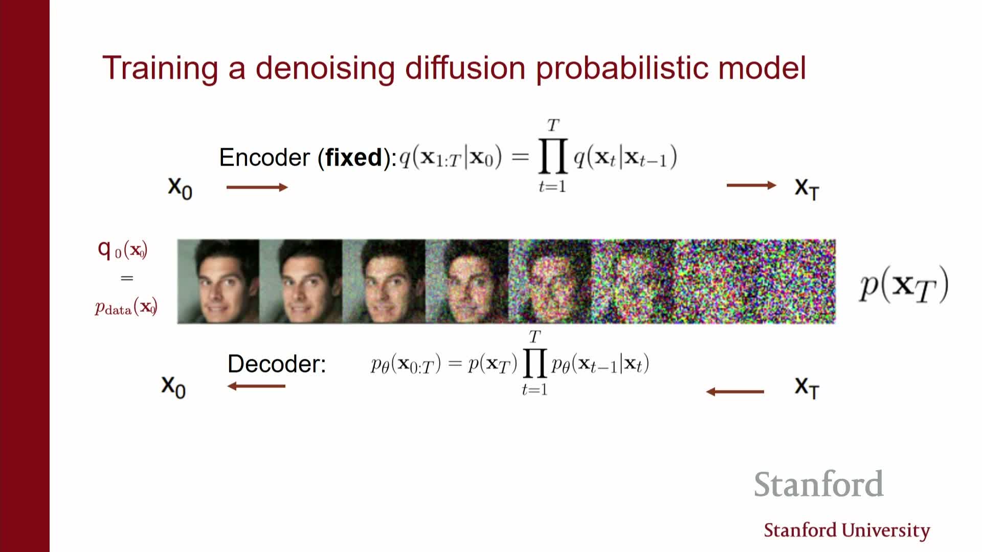
Score-based models and denoising diffusion probabilistic models (DDPMs) are two ways to define the same family of distributions obtained by progressively adding noise to data and learning a reverse process to remove that noise.
Key structure:
-
The forward (encoder) process is a sequence of Gaussian perturbations **q(x_t x_{t-1})** that gradually destroys data structure until pure noise is reached. -
The learned reverse (decoder) defines **p_θ(x_{t-1} x_t)**, typically parameterized as Gaussians whose means are predicted by neural networks.
Optimization link:
- Optimizing the variational ELBO for DDPMs reduces, after algebra, to matching the reverse decoders to the forward noising transitions.
- This matching is equivalent to learning denoisers or score functions at each noise level.
Consequence:
- Training either framework yields a sequence of denoisers: in DDPMs these are discrete-step decoders, and in score-based models they are noise-conditional score estimators.
ELBO training reduces to learning a sequence of denoisers and score functions
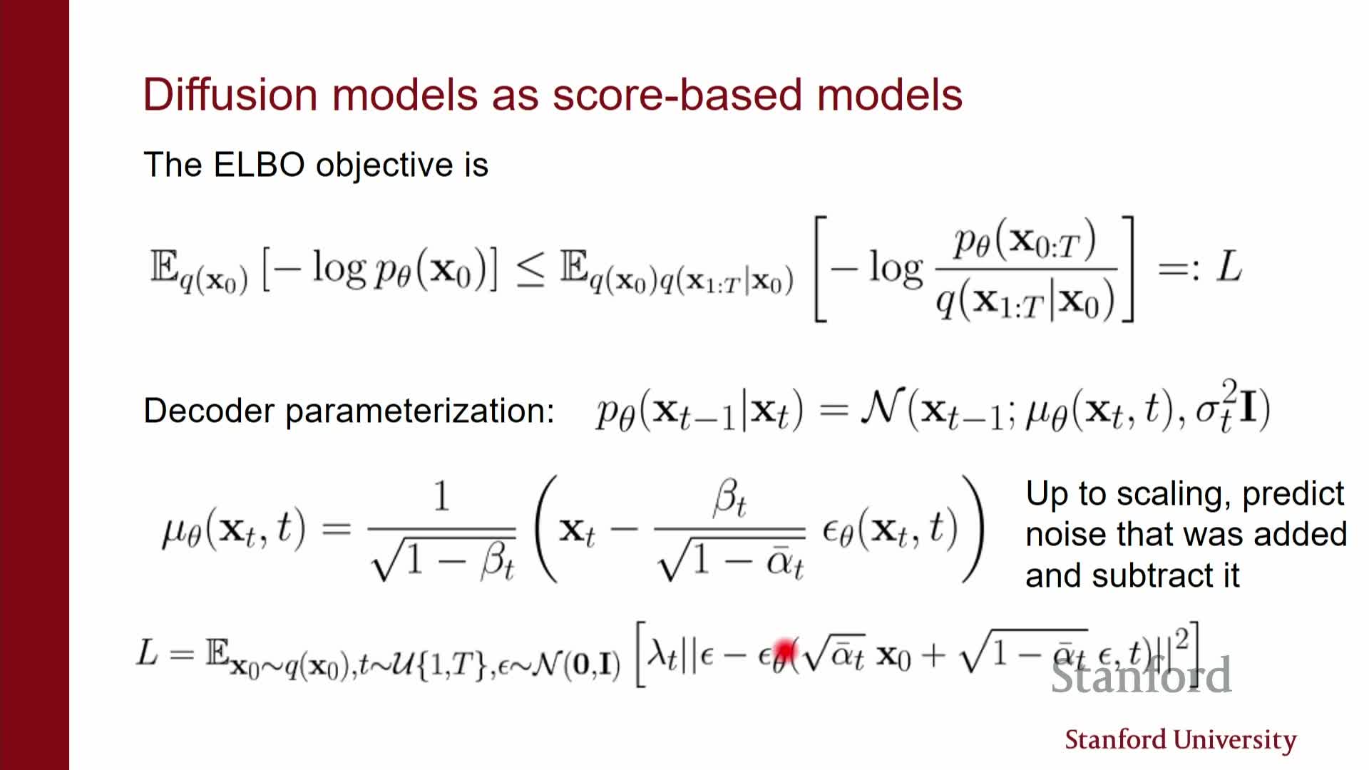
The variational ELBO for diffusion models decomposes into terms that are KL divergences between the forward noising path and the modelled reverse path.
Important simplifications:
- These KL terms simplify to denoising or score-matching objectives at individual noise levels.
-
Learning the optimal reverse conditional **p_θ(x_{t-1} x_t)** therefore amounts to estimating the score of the perturbed-data density or equivalently training denoisers that map noisy inputs to cleaner reconstructions.
Discrete vs continuous:
- In the discrete DDPM setup you train a finite set of denoisers (one per step).
- In the continuous formulation you train a continuum of denoisers (scores indexed by time).
Why architectures and losses align:
- This formal equivalence explains why architectures and loss functions in score-based models and DDPMs are closely related.
- It also explains why sampling updates resemble Langevin-type gradient steps plus noise.
Continuous-time diffusion (the diffusion limit) generalizes discrete-step DDPMs
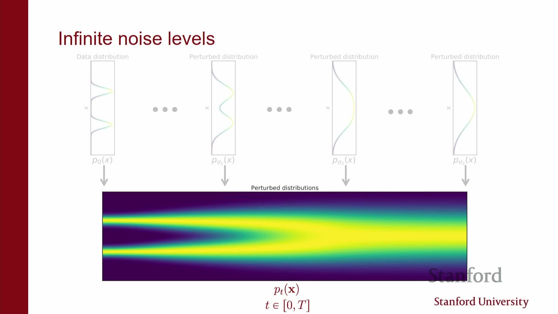
Taking the diffusion limit replaces the discrete sequence of noise levels with a continuum indexed by t ∈ [0, T], producing marginal densities p_t(x) that interpolate from data (t=0) to noise (t=T).
How this arises:
- Viewing forward noising as an infinitesimal limit of Gaussian perturbations leads to an SDE that describes how x_t evolves under infinitesimal drift and diffusion.
Practical benefits of the continuous view:
- Access to continuous-time tools: SDE/ODE solvers, Fokker–Planck analysis.
- Unified interpretation: DDPMs and score-based methods appear as discretizations of the same underlying process.
- Motivates more sophisticated numerical schemes and sampler designs because discrete DDPMs are time discretizations of the continuum.
The forward process is an SDE with drift and diffusion describing noise addition
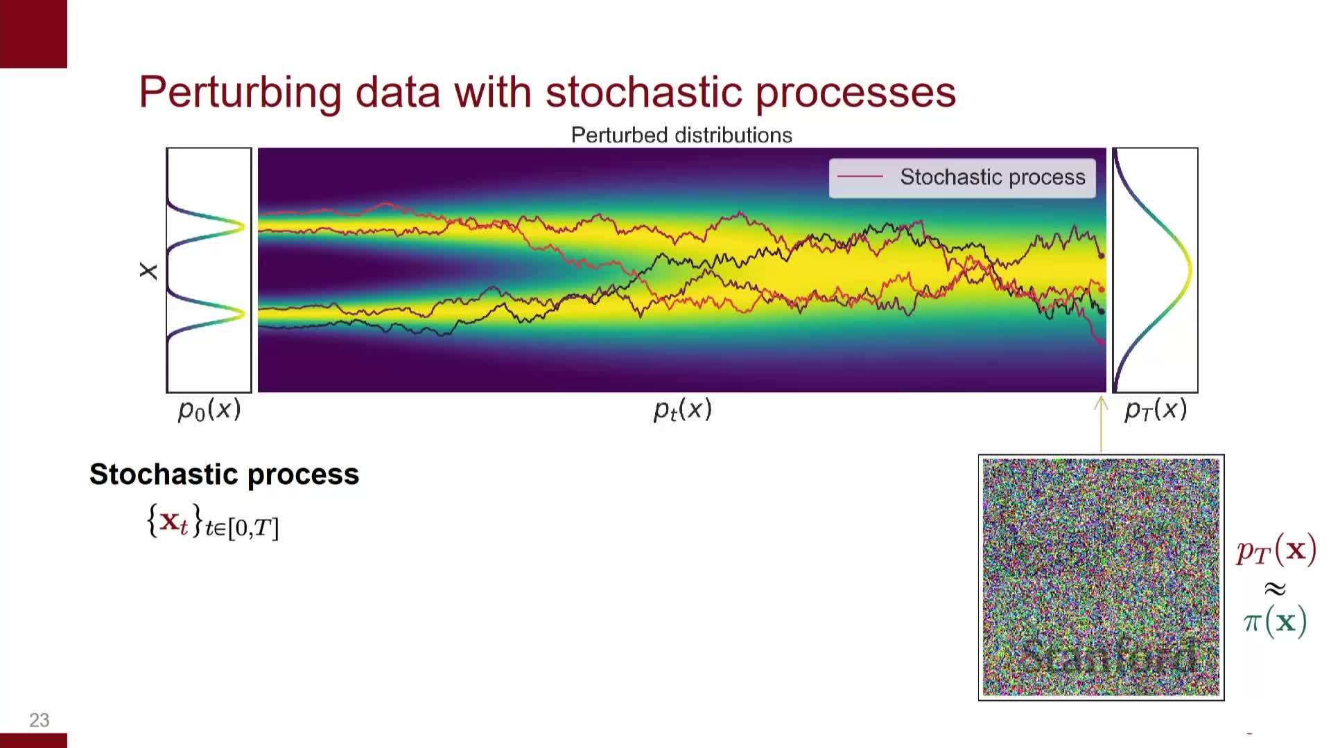
Formally the forward noising process can be written as an SDE: dX_t = f(X_t,t) dt + g(t) dW_t, where:
- f(X_t,t) is the drift field,
- g(t) scales the noise, and
-
dW_t is the Wiener increment (Brownian motion).
Key points:
- In the simple isotropic noising case f = 0, and the dynamics reduce to pure diffusion.
- The differential notation dX_t captures infinitesimal changes obtained by taking finer discretizations of the discrete chain; integrating these infinitesimal updates yields the observed smoothed densities p_t(x).
- Each marginal p_t(x) is a smoothed version of the data density because the forward SDE corresponds to incremental convolution with Gaussian kernels.
Why this matters:
- The SDE formalism provides the precise probabilistic object whose reverse-time dynamics will be used for generative sampling.
Reverse-time SDE introduces a score-dependent drift used for sampling
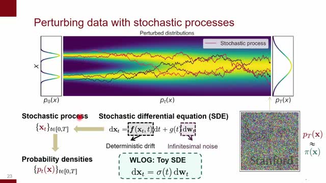
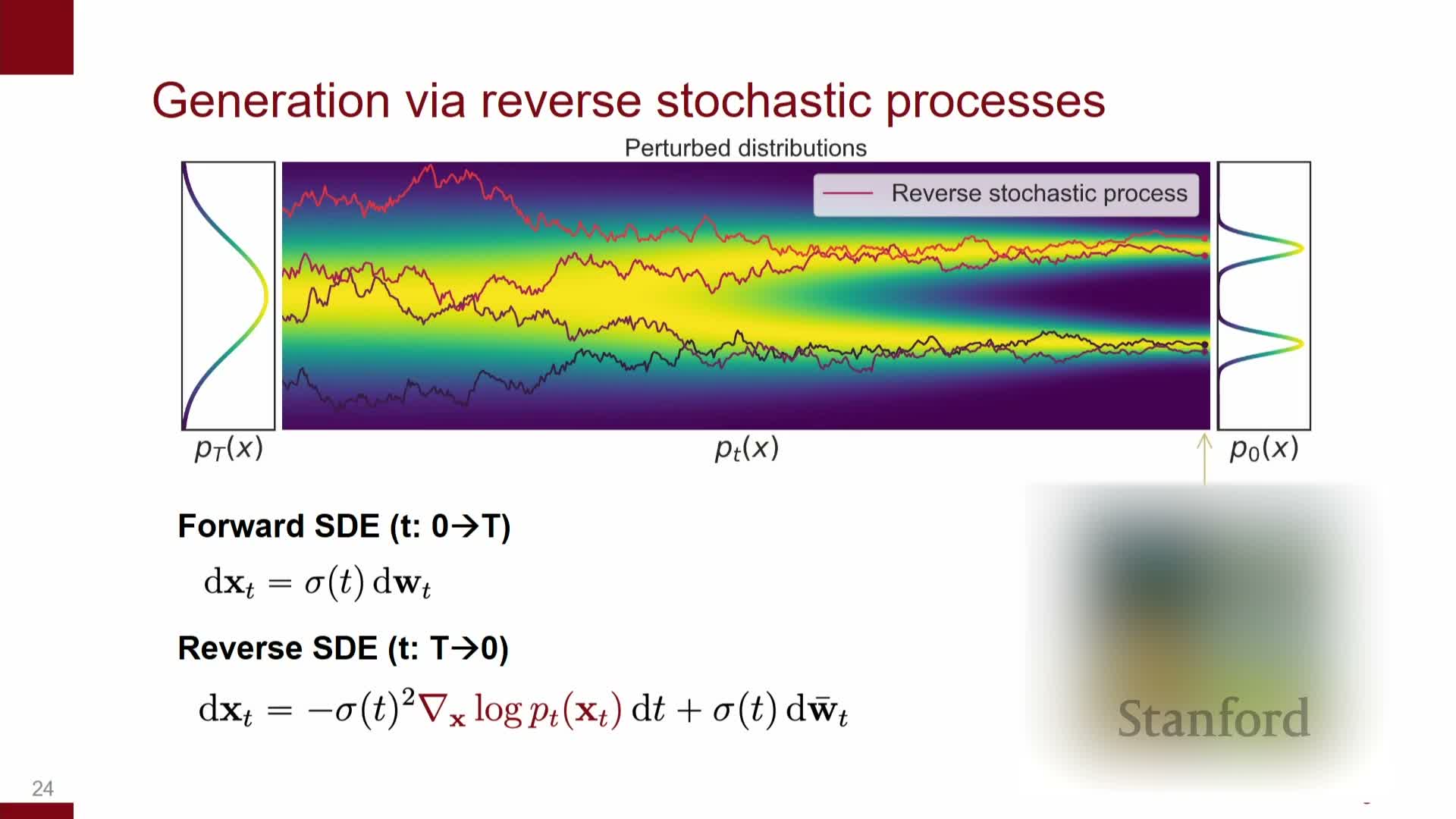
Reversing the forward SDE in time yields another SDE whose drift depends on the score (the gradient of log density) of the forward marginal p_t(x).
Intuition and sampling procedure:
- The score term provides the structured velocity field needed to move samples from noise toward regions of high data probability.
- To sample from the data distribution, initialize x_T from the simple prior and integrate the reverse SDE toward t = 0.
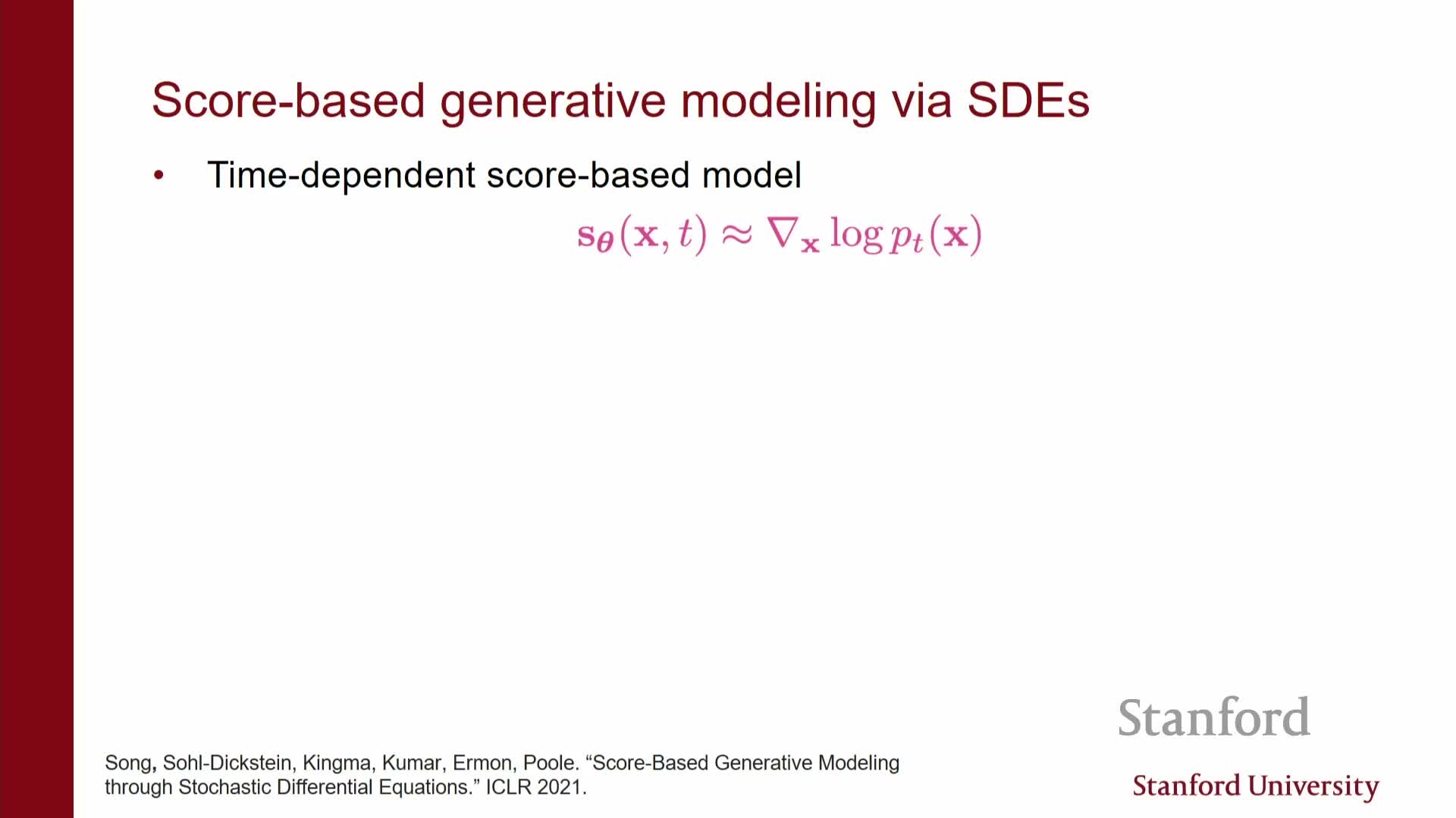
- Doing this requires access to the time-dependent score s(x,t) = ∇_x log p_t(x).
Notes on drift:
- When the forward SDE has zero drift, the reverse SDE’s drift is exactly the score term.
- If the forward SDE includes drift, that drift must be transformed appropriately in the reverse dynamics.
Practical implication:
- The need to know s(x,t) motivates training neural networks to estimate it by score matching so the reverse SDE can be simulated approximately during inference.
Score estimation and discretization yield DDPM-like denoising updates
The score-based training objective estimates the continuum family of scores s(x,t) for all t using noise-conditional score matching losses, which regress model scores to true scores in an L2 sense under perturbed-data distributions.
From training to sampling:
- Plugging estimated scores into the reverse SDE and discretizing time gives iterative update rules that are algebraically equivalent to the denoising and Langevin-style steps used in DDPMs: at each discrete time step, follow the estimated score and add a controlled noise term.
Discretization trade-offs:
- More steps → smaller numerical error, closer to continuous reverse flow.
- Fewer, larger steps → faster, but introduce bias.
Hybrid samplers:
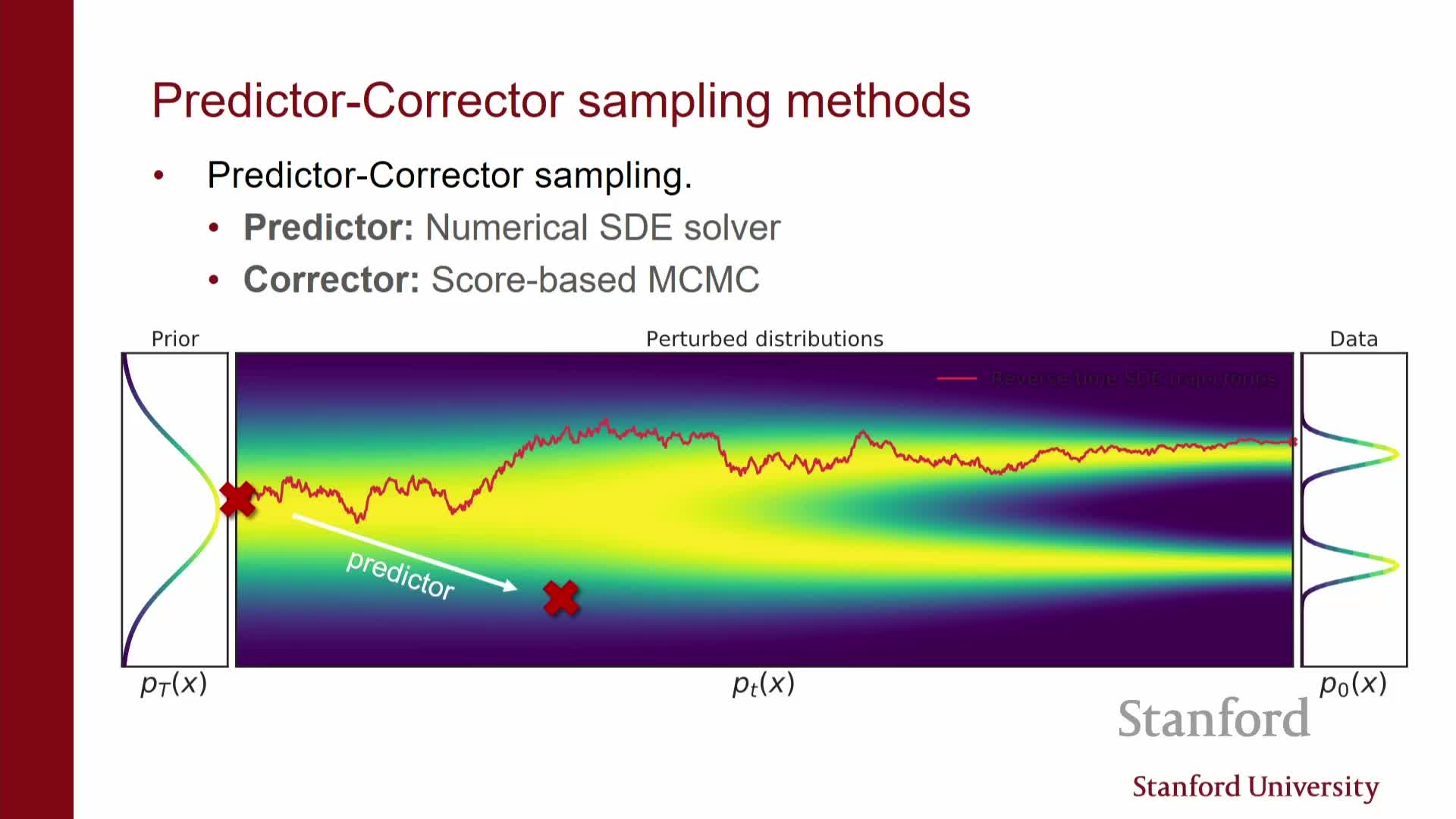
- Combining a predictor (deterministic step) and a corrector (stochastic refinement) yields hybrid samplers that trade compute for sample accuracy.
An equivalent deterministic ODE (flow) exists with identical marginals
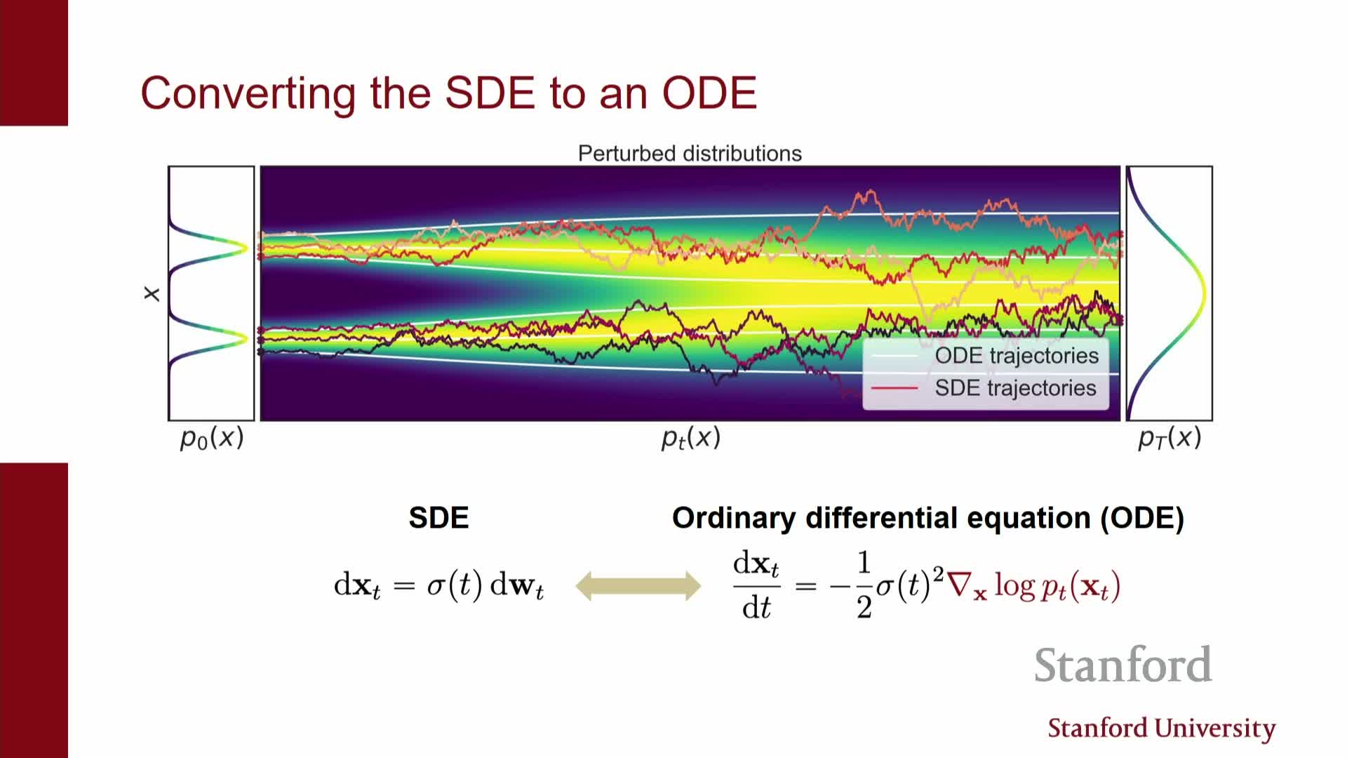
Under mild conditions the stochastic reverse dynamics can be reparameterized into a deterministic ODE whose flow preserves the same family of marginal densities p_t(x) as the SDE.
Consequences and structure:
- The ODE removes per-step stochasticity and concentrates randomness into the initial condition.
- The ODE defines an invertible mapping between latent noise x_T and data x_0, so solving it forward or backward yields a continuous normalizing flow parameterized by the score or related network.
- This enables interpreting diffusion models as continuous-time normalizing flows and leveraging neural ODE machinery: the model becomes a neural ODE whose vector field is given by score-derived functions.
- The deterministic ODE has unique, non-crossing trajectories, ensuring invertibility and enabling exact change-of-variable computations for likelihoods given an exact score.
Likelihood evaluation via ODE change-of-variables uses trace-Jacobian integration
For the deterministic ODE formulation the likelihood of a data point can be computed by mapping it to the latent noise space via solving the ODE backward and applying the continuous change-of-variables formula.
Concretely:
- The log-likelihood obeys log p(x_0) = log p(x_T) + ∫_0^T -Tr(∂f/∂x)(x_t,t) dt, where f is the ODE vector field and Tr(∂f/∂x) is the trace of its Jacobian.
- The integral can be evaluated alongside ODE integration using black-box ODE solvers and stochastic trace estimators when dimensions are large.
Practical notes:
- Numerical ODE solver technology gives access to adaptive step-size control, higher-order methods, and other techniques to improve sampling speed and accuracy.
- This perspective enables competitive likelihood estimation even when training used score-matching rather than maximum likelihood.
- Computing likelihoods requires integrating and potentially differentiating through the ODE solver for training-time likelihood optimization (numerically intensive), but evaluation alone is practical.
Sampling tradeoffs: ODEs give faster deterministic samples while SDEs provide robustness
Trade-offs between ODE and SDE samplers:
- ODE (deterministic) samplers: faster, noise-free generation, can use large adaptive steps, and enable exact likelihood computation if the score is exact.
- SDE (stochastic) samplers and predictor-corrector hybrids: maintain stochasticity at each step, keeping inputs closer to the training distribution and often reducing compounding error—usually higher sample quality at greater compute cost.
Discretization bias is the central tradeoff:
- Coarse discretization (fewer, larger steps) → speed but greater numerical error.
- Fine discretization (many small steps) → accuracy but higher compute.
Hybrid approaches and MCMC-style refinements give a flexible accuracy-vs-cost spectrum for inference.
Accelerated sampling methods (DDIM and coarse discretization) reduce step count
Accelerated samplers exploit structure in diffusion dynamics to reduce required model evaluations from thousands to tens or hundreds while keeping acceptable sample quality.
Examples and techniques:
- DDIM (deterministic non-Markovian samplers): re-parameterizes steps to take larger jumps along a discretized approximation of the reverse dynamics.
- Closed-form solutions for linear components of the SDE allow coarser time grids and larger steps, dramatically reducing network calls.
Practical considerations:
- Coarse discretization yields large speed-ups but increases approximation error.
- Discretization granularity is a tunable knob traded against fidelity; advanced step selection and bespoke integrators further improve coarse-step samplers.
Parallel-in-time ODE solvers trade compute for wall-clock speed by denoising trajectory segments concurrently
Parallel-in-time techniques partition the ODE trajectory and use multiple accelerators to estimate trajectory segments concurrently instead of sequentially.
How it works and trade-offs:
- Relies on good initial guesses for trajectory segments and iterative refinement.
- Many GPUs refine different temporal windows in parallel, effectively denoising multiple timesteps at once.
- This reduces wall-clock latency at the expense of greater aggregate compute and communication overhead.
When it’s useful:
- Particularly effective for large models with stringent latency requirements and abundant parallel resources.
- Produces the same asymptotic solution as sequential integration but with much lower response time when engineered carefully.
Progressive distillation and consistency models compress multi-step samplers into very few steps
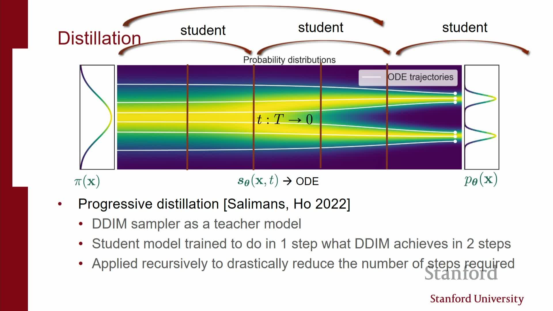
Progressive distillation compresses multi-step denoising into progressively fewer steps by training student networks to emulate a teacher’s multi-step behavior.
Procedure (high-level):
- Train a teacher that performs k denoising steps.
- Train a student to map the teacher’s state after k steps to the teacher’s state after 2k steps.
- Recursively repeat, halving the step budget each distillation round until a small-step or one-step sampler is obtained.
Outcomes and relatives:
- Produces exponential compression of the original step budget and dramatically reduces inference cost while preserving sample quality.
- Consistency models pursue a related objective by directly learning mappings from noisy inputs to denoised outputs that are consistent across step sizes; they enable one-shot or very low-step generation with specialized losses.
These distilled and consistency approaches are core to recent real-time text-to-image demos.
Latent diffusion uses a VAE-style encoder to reduce dimensionality and accelerate training and sampling
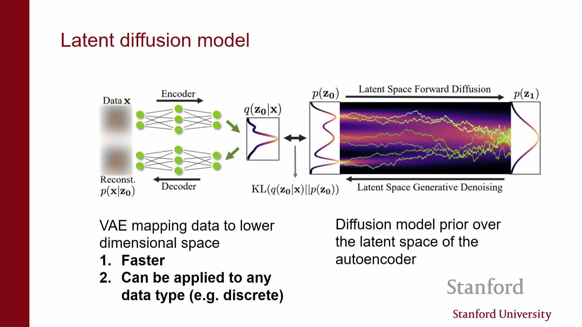
Latent diffusion models insert an encoder/decoder pair (VAE or autoencoder) upstream of the diffusion prior so the diffusion operates in a lower-dimensional continuous latent space rather than raw pixel space.
Why this helps:
- Pretraining the encoder/decoder to prioritize reconstruction quality lets the diffusion prior act on compact latent codes, reducing memory and compute costs while retaining perceptual fidelity via the decoder.
- Enables scaling diffusion models to very large datasets and high resolutions.
- Supports modalities where raw inputs are discrete (e.g., text) by first mapping to continuous latents.
Implementation notes:
- Often the encoder is pretrained and frozen for diffusion training, so the diffusion prior need not strictly match a Gaussian latent prior from the VAE; weak regularization suffices when the diffusion model acts as a powerful learned prior.
- This design underlies large-scale systems such as Stable Diffusion.
Conditional generation is implemented by supplying side information to the score/denoiser network
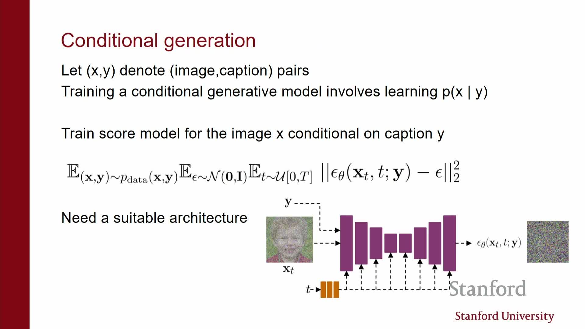
Conditional diffusion modeling of p(x | y) requires the score/denoiser to accept the conditioning variable y (class labels, captions, measurements) in addition to the noisy image x_t and time t.
Architectural choices for injecting y:
- Concatenation of embeddings with inputs,
- FiLM layers (feature-wise linear modulation),
- Cross-attention between image latents and text embeddings.
Effect on sampling:
-
The conditional score **s(x,t y)** steers reverse dynamics toward regions of the data manifold compatible with y, enabling conditional sampling by integrating the conditional SDE/ODE. - Proper handling of the conditioning signal at each noise level is essential because the denoiser must reason about both noisy inputs and the desired conditioning simultaneously.
Bayesian conditioning via classifier guidance: posterior scores equal prior plus likelihood score
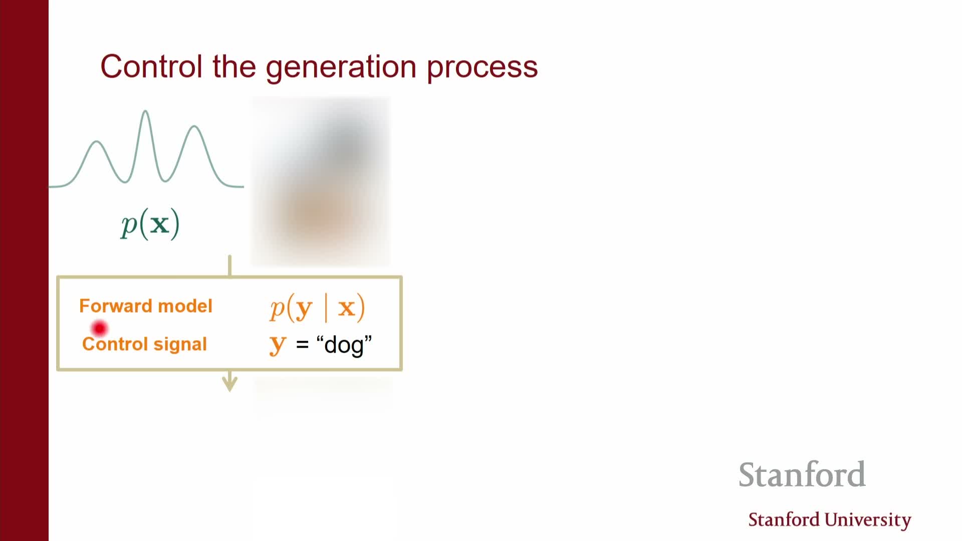
By Bayes’ rule p(x | y) ∝ p(x) p(y | x), and taking gradients of log densities yields the posterior score as the sum of the prior score and the likelihood score:
-
**∇_x log p(x y) = ∇_x log p(x) + ∇_x log p(y x)**.
Practical use:
- This identity lets you perform conditional sampling without retraining a conditional diffusion model by augmenting the prior score estimator with gradients from a classifier or a differentiable likelihood term.
- The intractable normalization constant disappears under gradient differentiation, making score-level Bayes conditioning tractable so long as gradients of the likelihood or classifier w.r.t. inputs are available.
| This provides a principled method to steer unconditional generative models toward desired attributes defined by **p(y | x)**. |
Classifier guidance and classifier-free guidance provide practical conditioning mechanisms
Classifier guidance uses an external classifier to compute ∇_x log p(y | x) and adds this term to the prior score during sampling, but the classifier must be evaluated on noisy inputs x_t or be adapted to those noise levels.
Classifier-free guidance sidesteps a separate classifier by training a single diffusion model on both conditional and unconditional data, then forming an implicit classifier by taking a scaled difference between conditional and unconditional score estimates during sampling.
Comparison and practice:
- Both approaches approximate the posterior score and allow controllable sampling without computing normalization integrals.
- Classifier-free guidance is often preferred for pipeline simplicity and empirical sample quality.
- These guidance techniques are used for editing, conditional synthesis, and inverse problems by defining the likelihood term appropriately.
Applications include image editing, inverse problems, and medical imaging where likelihoods encode measurement physics
The score-based Bayes conditioning framework naturally handles inverse problems where the likelihood p(y | x) describes a measurement process (e.g., MRI acquisition).
How it applies:
- Adding the measurement gradient to the prior score yields principled posterior sampling for reconstruction and uncertainty quantification.
- For interactive editing, conditioning signals can be sparse (sketches, strokes), and the forward model plus denoiser produce coherent conditioned images by following the posterior score during reverse sampling.
- Text-to-image: a caption embedding serves as y and conditions the denoiser, typically implemented via cross-attention between image latents and text embeddings.
Deployment trade-offs:
- Balance conditioning strength, computational budget, and the fidelity of pretrained encoders/classifiers used in the guidance term.
Classifier-free guidance and other practical tricks avoid explicit classifier training
Classifier-free guidance achieves the effect of classifier guidance by training a model that sometimes sees conditioning y and sometimes sees none, then computing a guidance vector as the difference between conditional and unconditional score outputs scaled by a guidance weight at sampling time.
Practical alternatives and tricks:
- Estimating gradients w.r.t. noisy inputs, using learned guidance models, or approximating likelihood gradients through surrogate models.
- These variants aim for stability and scalability in large models.
Empirical preference:
- Simple, robust conditioning procedures like classifier-free guidance are favored because they integrate easily into existing diffusion architectures and scale to large datasets.
Recent engineering advances yield real-time or very low-step generation by combining distillation, latent models, and advanced solvers
State-of-the-art systems achieve real-time or near-real-time text-to-image synthesis by composing several advances:
- Latent diffusion (operate in compact latent spaces)
- Large pretrained text encoders (strong conditioning representations)
- Progressive distillation (compress many steps into a few)
- Optimized ODE/SDE solvers including parallel-in-time algorithms
Practical outcome:
- Groups like Stability AI combine these elements to trade aggregate compute for low wall-clock latency while preserving perceptual quality.
- The continuous-time perspective unifies these techniques and enables principled derivation of new solvers, consistency objectives, and distillation strategies that further reduce inference cost.
Result: a rich toolbox for selecting trade-offs between sample quality, compute, and latency tailored to application constraints.
Summary: score estimation unlocks multiple inference paradigms and practical tradeoffs
Estimating the time-dependent score function is the central learning problem that enables multiple inference paradigms:
- Stochastic reverse SDE sampling (robust, high quality)
- Deterministic ODE flow sampling (fast transforms, likelihoods)
- Accelerated coarse-step samplers (fewer evaluations)
- Conditional generation via score-level Bayes manipulation (guided sampling)
Each paradigm presents a different accuracy-compute trade-off:
- SDEs: robustness and high quality
- ODEs: faster deterministic transforms and likelihood evaluation
- Distillation/consistency models: compress multi-step dynamics into few- or single-step generation
Latent diffusion models reduce dimensionality to scale, while classifier-free guidance and other conditioning tricks make controlled generation practical at scale.
Together, these techniques form a unified framework for modern diffusion-based generative modeling, spanning theory to high-performance engineering.
Enjoy Reading This Article?
Here are some more articles you might like to read next: