Stanford CS236- Deep Generative Models I 2023 I Lecture 18 - Diffusion Models for Discrete Data
- Lecture introduction and topic overview
- Generative modeling framing and predominance of continuous image data
- Motivation for discrete generative modeling
- Why continuous generative methods do not trivially extend to discrete data
- Problems with embedding discrete tokens to continuous spaces
- Autoregressive models as the standard discrete probabilistic approach
- Limitations of autoregressive modeling
- Score matching perspective and research question
- Finite-difference gradient and the concrete score
- Restricting ratios to single-position neighbors to control complexity
- Parameterizing local ratios with sequence neural networks
- Learning the concrete score via a score-entropy loss
- Optimization strategies: implicit and denoising score entropy
- Practical training procedure using a perturbation kernel
- Modeling discrete diffusion as a continuous-time Markov process
- Computing intermediate densities via matrix exponentiation
- Uniform and absorbing (mask) transition examples and implications
- Time-dependent concrete score estimation for p_t ratios
- Reverse diffusion and relation between forward and reverse generators
- Sampling from the reverse process using the learned concrete score
- Computational bottleneck of single-token jumping and simultaneous-step acceleration
- End-to-end pipeline and illustrative text generation
- Quality-versus-compute trade-off and comparison to autoregressive models
- Controllable generation and flexible conditioning (prompting and infill)
- Likelihood evaluation and a perplexity upper bound via denoising score entropy
- Empirical likelihood and perplexity comparisons to autoregressive baselines
- Summary and concluding observations
Lecture introduction and topic overview
The lecture introduces diffusion models for discrete data, with an emphasis on applications to language and a guest lecture contributor who has done foundational research in discrete diffusion approaches.
The objective is to adapt diffusion-based generative modeling—traditionally applied to continuous data like images—to discrete modalities such as text.
The talk sets expectations to cover:
-
Theoretical generalizations of diffusion to discrete spaces
-
Algorithmic constructs for learning and sampling discrete diffusions
-
Empirical comparisons to autoregressive language models
Generative modeling framing and predominance of continuous image data
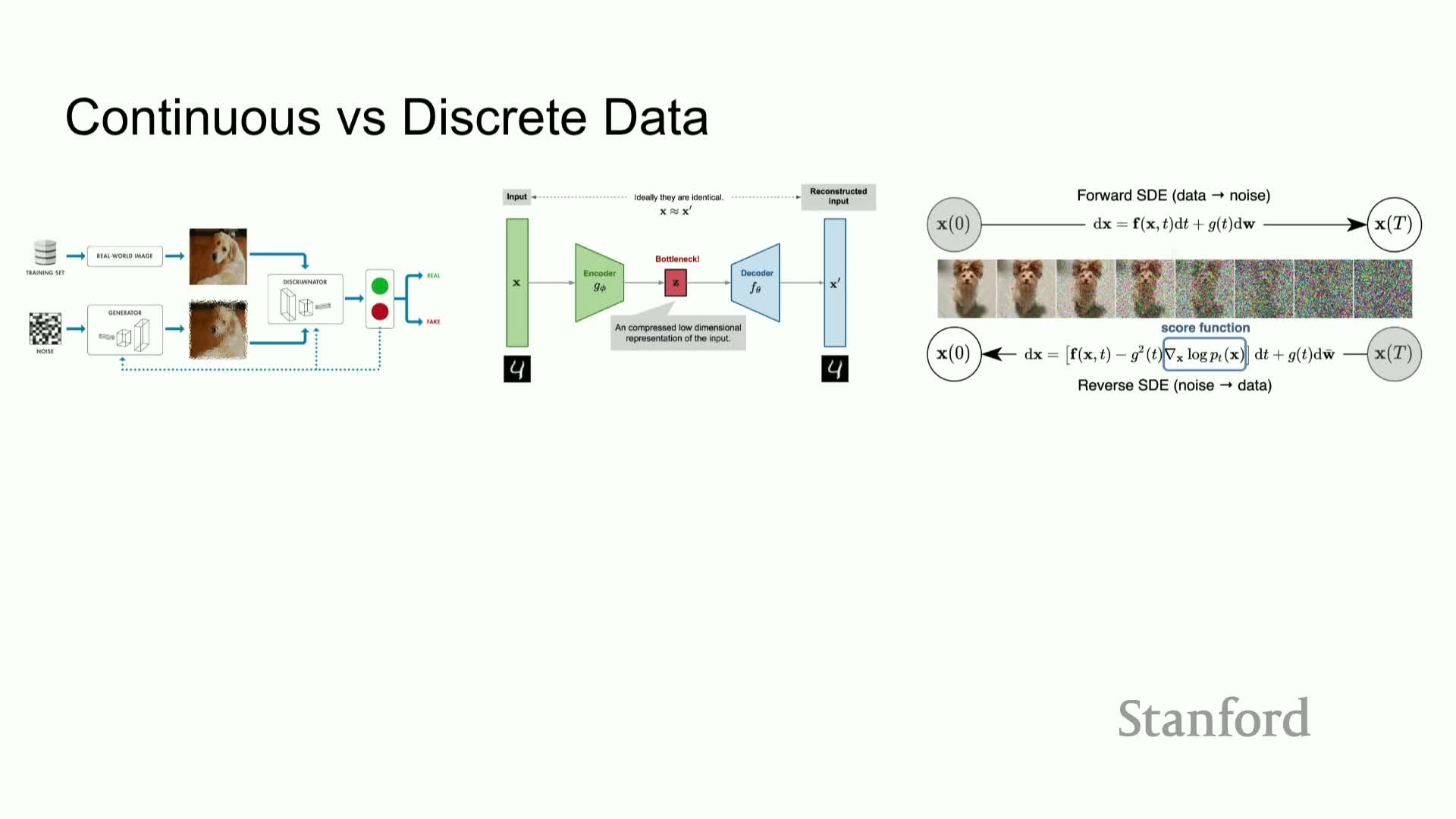
Generative modeling is posed as learning a parameterized distribution P_θ to approximate an unknown data distribution P_data from i.i.d. samples, enabling synthesis of new samples when successful.
The lecture highlights why many standard generative paradigms (GANs, VAEs, flows, diffusion) are illustrated with images:
- Images live in a continuous R^d pixel space that supports interpolation and smooth transformations.
- That continuous structure underlies algorithmic tools assuming differentiability and continuity, which explains why image-centric methods have dominated prior work.
Motivation for discrete generative modeling
Discrete data domains such as natural language, DNA, and discretized image latents are ubiquitous and scientifically important, motivating probabilistic models that natively handle discrete tokens.
Key points:
-
Language modeling and large-scale pretraining explicitly model distributions over discrete token sequences, making discrete generative models directly applicable and often preferable.
- Applications include:
-
Language generation
-
Molecular design (sequence-based representations)
-
VQ-style image latents
-
Language generation
- Discrete generative models are essential for sampling valid sequences and discovering novel structured objects in these domains.
Why continuous generative methods do not trivially extend to discrete data
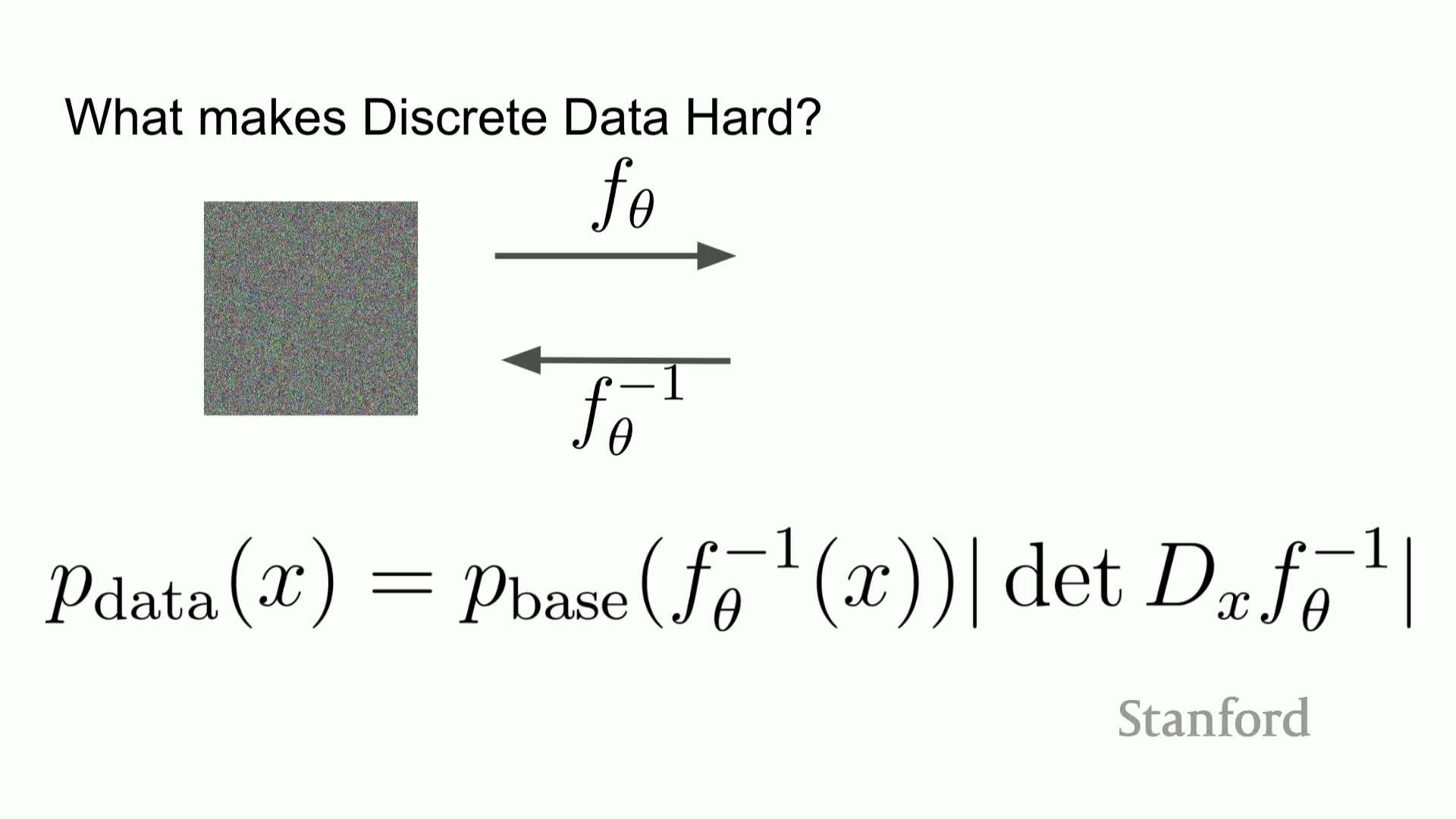
Many continuous generative methods rely on calculus and smooth change-of-variables operations that do not hold in discrete spaces, so naive adaptations fail.
Concrete failure modes:
- For normalizing flows, the change-of-variables formula requires bijective differentiable transforms and continuous Jacobians; discretizing breaks those properties and forces the base distribution to be as expressive as the data distribution.
- For GANs, discrete outputs block gradient backpropagation through sampling because derivatives are undefined, so standard adversarial training does not apply without additional estimators or relaxations.
Problems with embedding discrete tokens to continuous spaces
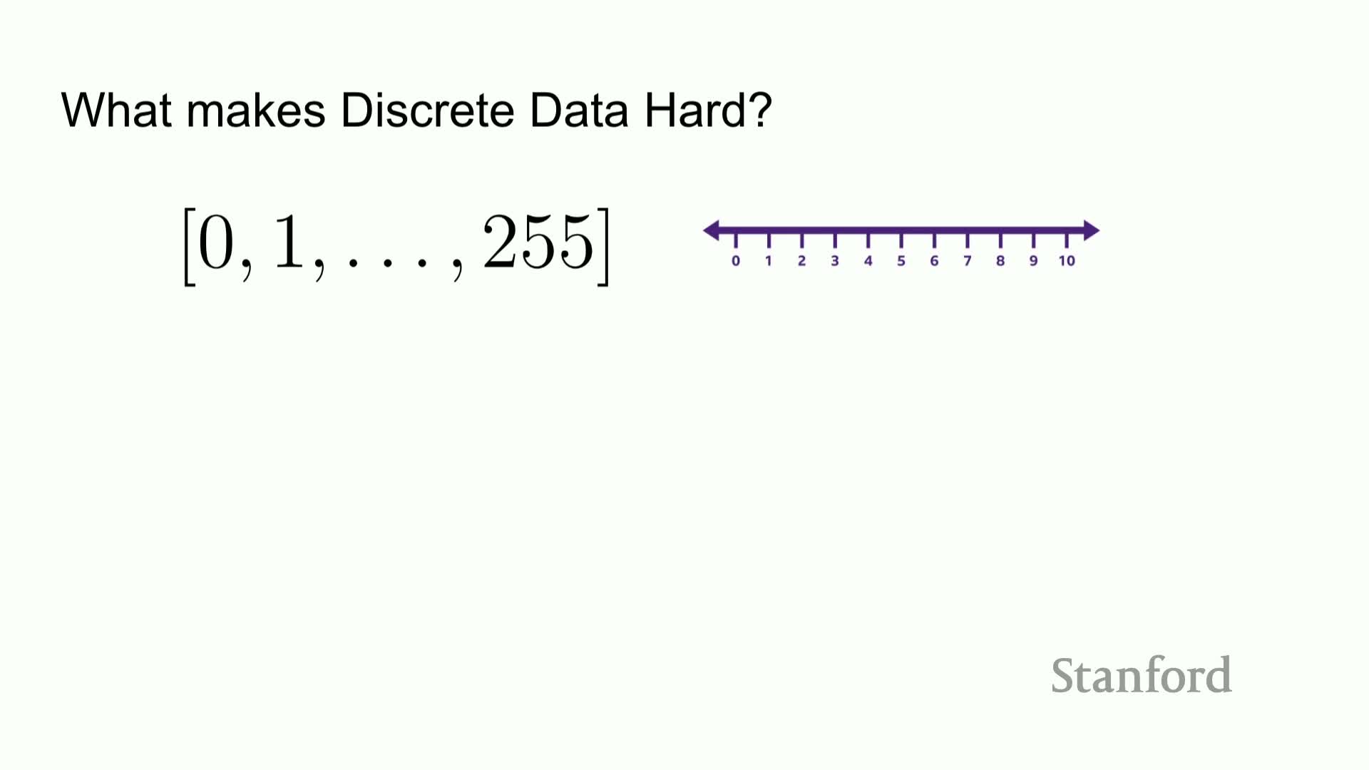
Embedding discrete tokens into continuous spaces and then rounding generated vectors back to tokens creates problems:
- It introduces large regions of empty space and unreliable discretization behavior.
- While rounding can work for low-resolution image ranges (e.g., 0–255), token embedding spaces are high-dimensional and sparse, so sampling near but not exactly at an embedding often maps to semantically inappropriate tokens.
Consequences:
- Continuous-token pipelines become brittle: small modeling errors lead to invalid discretizations and poor generative quality.
- Methods that rely on near-perfect continuous generation are impractically sensitive to error accumulation.
Autoregressive models as the standard discrete probabilistic approach
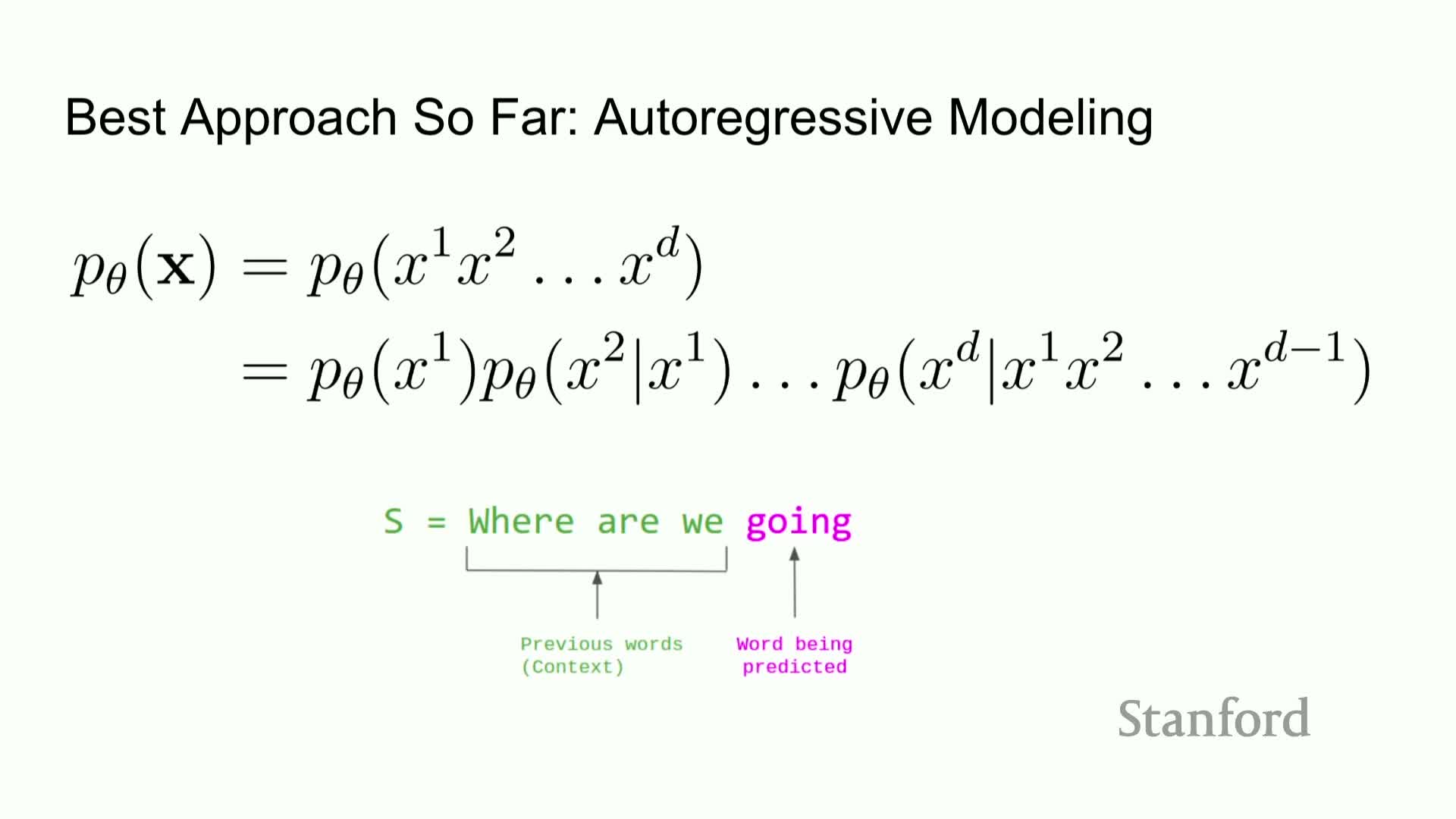
Autoregressive decomposition factorizes the joint probability of a token sequence into conditional token probabilities and estimates each conditional with a network (e.g., Transformer).
Reasons this approach is dominant:
- Scalability: each next-token distribution is computed over the vocabulary.
- Expressivity: with sufficient capacity it can represent any sequence distribution in principle.
- Alignment with generation: it matches the left-to-right generative process of natural language.
- Training and evaluation: yields a straightforward maximum-likelihood objective and tractable exact sequence likelihoods.
Limitations of autoregressive modeling
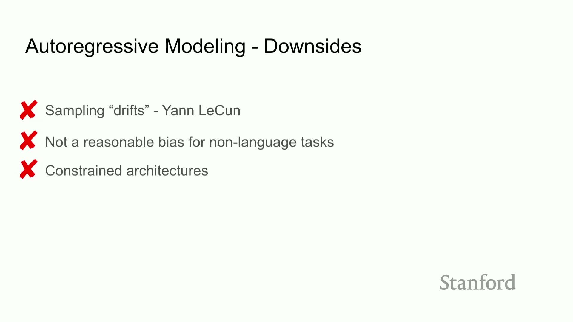
Limitations of autoregressive sampling:
-
Error accumulation during sequential sampling can cause generation drift.
- Imposes a left-to-right inductive bias that may be unnecessary or suboptimal for many discrete domains.
- Inherently sequential and therefore slow at sampling time.
- Architectural constraints (e.g., causal attention masks) add modeling restrictions and complicate flexible conditioning or in-filling.
These limitations motivate exploring alternative discrete generative paradigms that can generate tokens in parallel and provide different inductive biases.
Score matching perspective and research question
Score matching offers an alternative by modeling gradients of the log density rather than the density itself, which circumvents the need to normalize across an exponentially large discrete sample space.
Central research question posed: can score-based techniques and diffusion-style generative frameworks be generalized to discrete spaces to yield practical discrete generative models?
This motivates deriving discrete analogues of the score function and corresponding learning and sampling procedures.
Finite-difference gradient and the concrete score
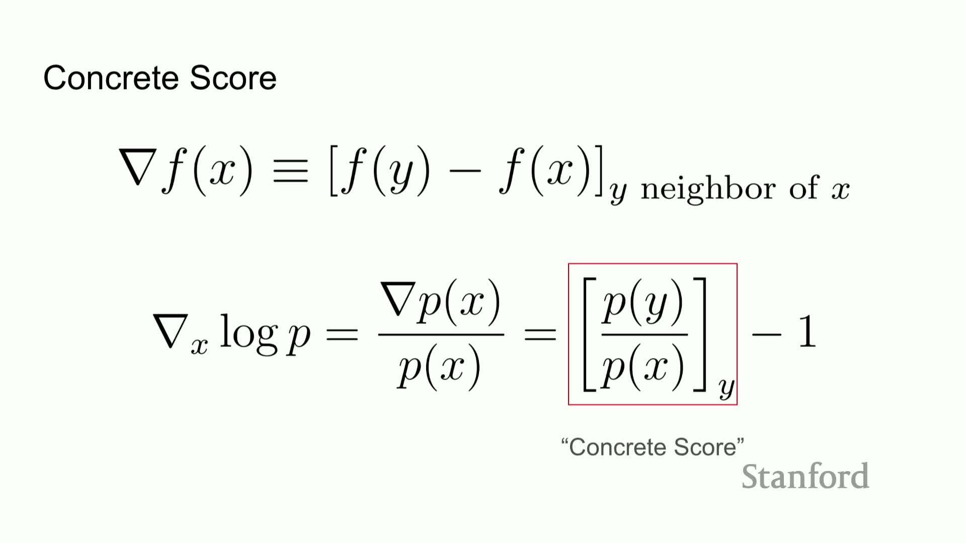
The continuous score (gradient of log probability) generalizes to discrete finite differences:
- Replace derivatives by differences f(y) − f(x) over neighboring states to obtain a discrete analogue of a gradient.
Applied to log-probabilities, this produces a collection of density ratios p(y)/p(x) indexed over neighbors y of x. That object is termed the concrete score and serves as the discrete counterpart to the continuous score function.
The concrete score captures local relative probabilities and is the fundamental quantity to estimate for discrete score-based modeling.
Restricting ratios to single-position neighbors to control complexity
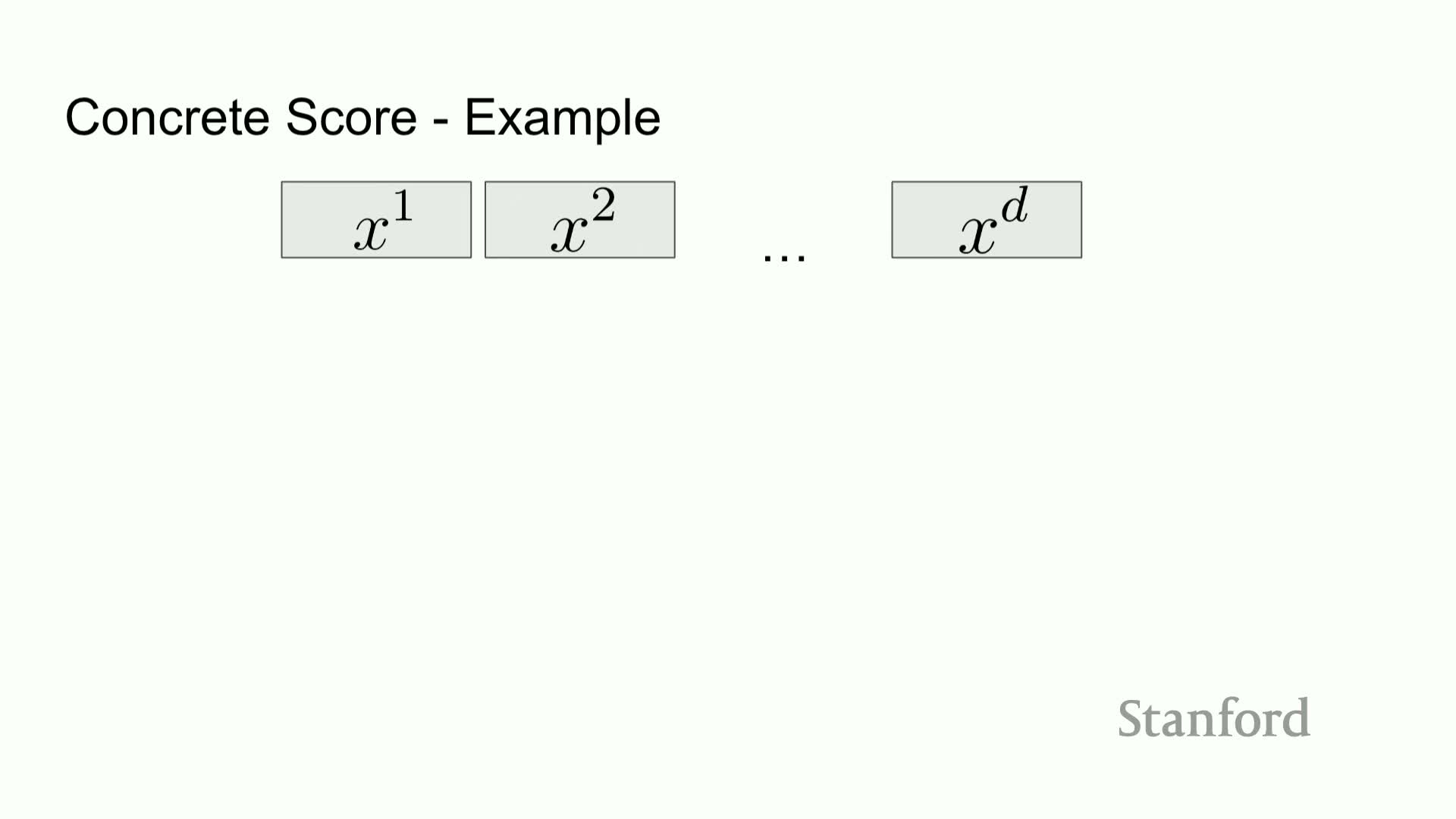
Modeling all p(y)/p(x) ratios for arbitrary y is computationally prohibitive because the number of pairs is exponential in sequence length.
Practical restriction:
- Focus on ratios between sequences that differ at a single token position, yielding a locality constraint.
Benefits: - Reduces computational complexity to O(N * D) for vocabulary size N and sequence length D.
- Preserves expressivity for learning local transition behavior while keeping estimation and representation tractable for neural parameterization.
Parameterizing local ratios with sequence neural networks
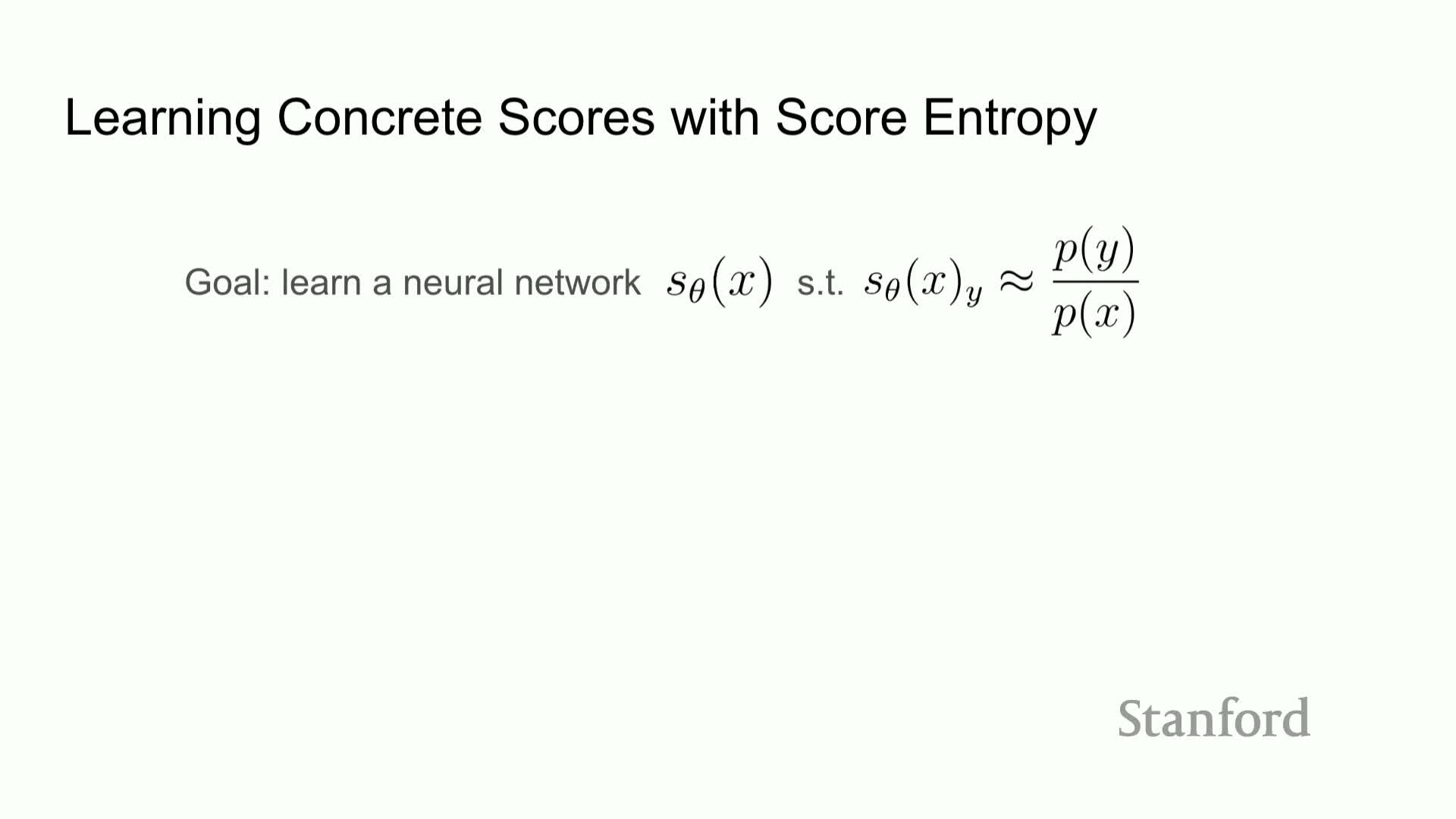
Local density ratios can be parameterized by feeding the full token sequence into a sequence model that outputs per-position ratio vectors across the vocabulary.
Design highlights:
- Uses a parallel, non-autoregressive architecture: the network produces conditional scores for every position simultaneously rather than iterating left-to-right.
- Implementationally resembles a non-causal Transformer which outputs D separate conditional distributions (ratio vectors) corresponding to flipping each token independently.
Learning the concrete score via a score-entropy loss
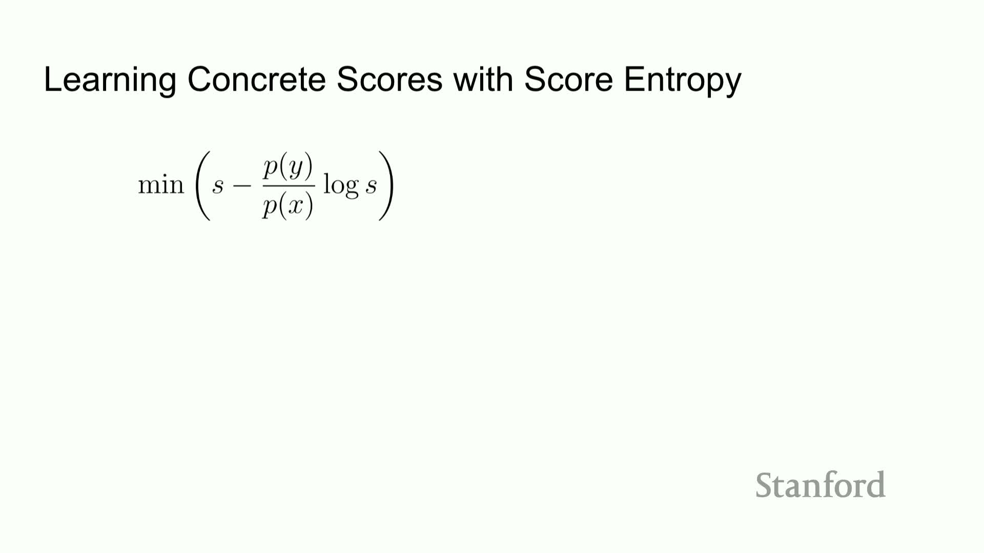
A principled loss named score entropy generalizes continuous score-matching objectives to discrete ratios.
Properties of score entropy:
- Measures a divergence between the modeled ratio outputs and the true p(y)/p(x) ratios summed over neighbors and averaged under the data distribution.
- Minimizing the score-entropy loss yields consistent recovery of the true discrete ratios under sufficient model capacity and data.
- The loss is convex in the log-ratio parameterization, giving well-behaved optimization properties.
Score entropy serves as the principal objective for fitting the concrete score network.
Optimization strategies: implicit and denoising score entropy
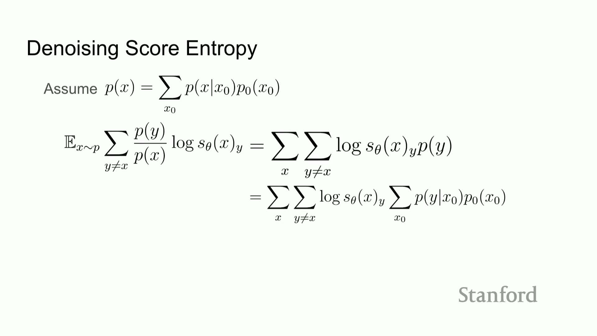
Direct evaluation of the score-entropy loss requires unknown true ratios p(y)/p(x), so two practical strategies are proposed:
-
Implicit score entropy: an implicit-estimation generalization (details omitted here), and
-
Denoising score entropy: a denoising-based estimator that makes the objective computable.
Denoising score entropy assumes the data distribution is a convolution of the true data with a tractable perturbation kernel, allowing unknown terms to be rewritten as expectations over the corruption process—analogous to continuous denoising score matching.
Practical training procedure using a perturbation kernel
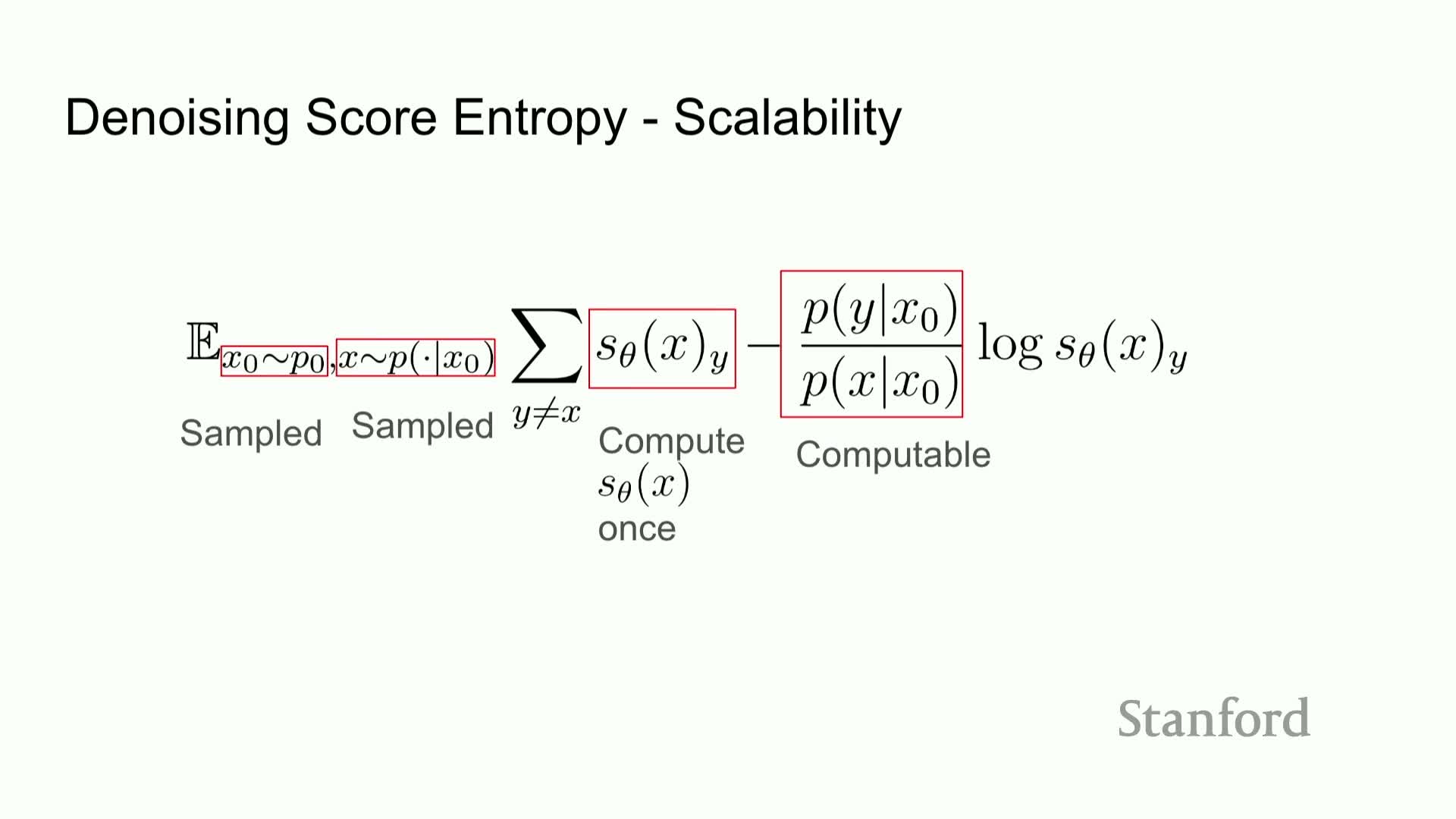
Under the denoising reduction, training proceeds as follows:
- Sample a clean sequence x0 from the data.
-
Sample a corrupted sequence xt from a tractable perturbation kernel p(xt x0).
- Minimize the denoising score-entropy loss comparing the model output to transition ratios computable from the kernel.
| Because the corruption kernel is tractable, the intractable p(y)/p(x) terms are replaced by computable ratios p_t(y | x0) / p_t(x | x0), making minibatch stochastic optimization feasible. |
This mirrors continuous denoising score matching and provides a scalable training recipe.
Modeling discrete diffusion as a continuous-time Markov process
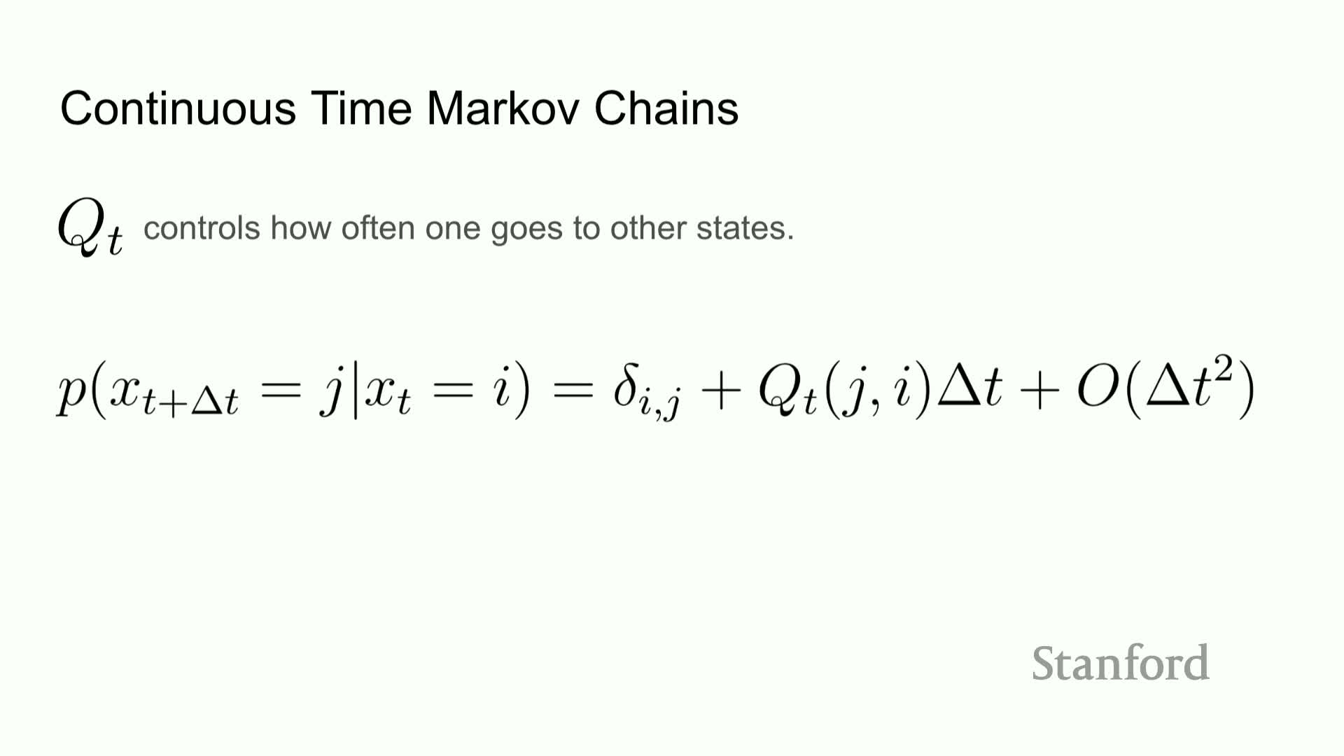
Discrete diffusion is expressed as the linear Kolmogorov forward equation on the probability vector p_t, governed by a rate matrix Q_t that controls jump rates between discrete states.
Mathematical constraints on Q_t:
- Off-diagonal entries must be nonnegative (rates).
- Columns must sum to zero to preserve total probability.
Exponentiating Q_t Δt yields finite-time transition kernels. This continuous-time Markov chain formalism is the natural discrete analogue to continuous diffusion SDEs and provides a principled forward-noising process.
Computing intermediate densities via matrix exponentiation
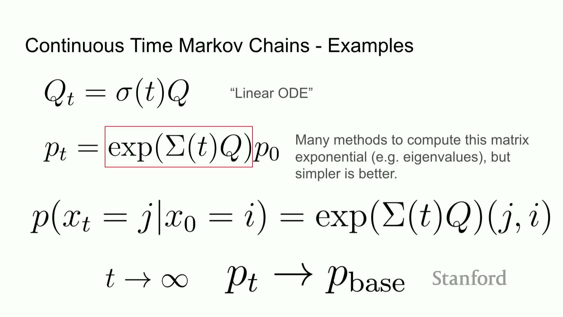
Given a rate matrix Q and initial probability vector p0, intermediate densities p_t can be computed via matrix exponentiation p_t = exp(t Q) p0, which exactly solves the linear ODE.
Practical considerations:
- Use scalable approximations of the matrix exponential or exploit structure in Q to avoid explicit large-matrix operations.
- The exponentiated kernel yields intuitive behavior: mass leaves states at rates given by diagonal entries and enters others via off-diagonals; as t → ∞ the chain approaches the designated base distribution.
Uniform and absorbing (mask) transition examples and implications
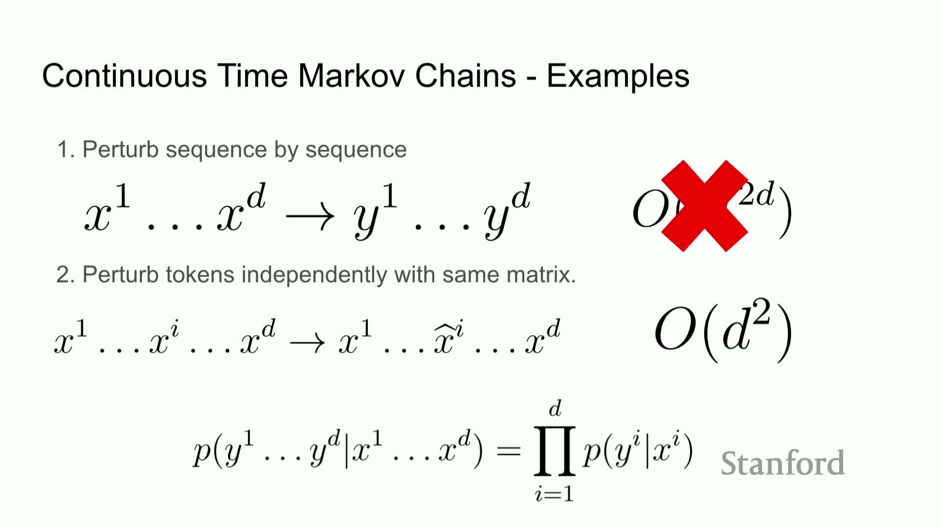
Two canonical Q choices illustrate distinct noising behaviors:
-
Uniform transition Q: each token jumps to any other token uniformly, driving the distribution towards uniformity as t increases.
-
Absorbing-mask Q: tokens transition to a special mask state, driving sequences to masked forms.
These options define different forward-noise geometries with distinct inductive biases:
- Uniform noise randomizes broadly.
- Masking preserves structural coherence by collapsing tokens to a neutral placeholder that is easier to denoise.
Time-dependent concrete score estimation for p_t ratios
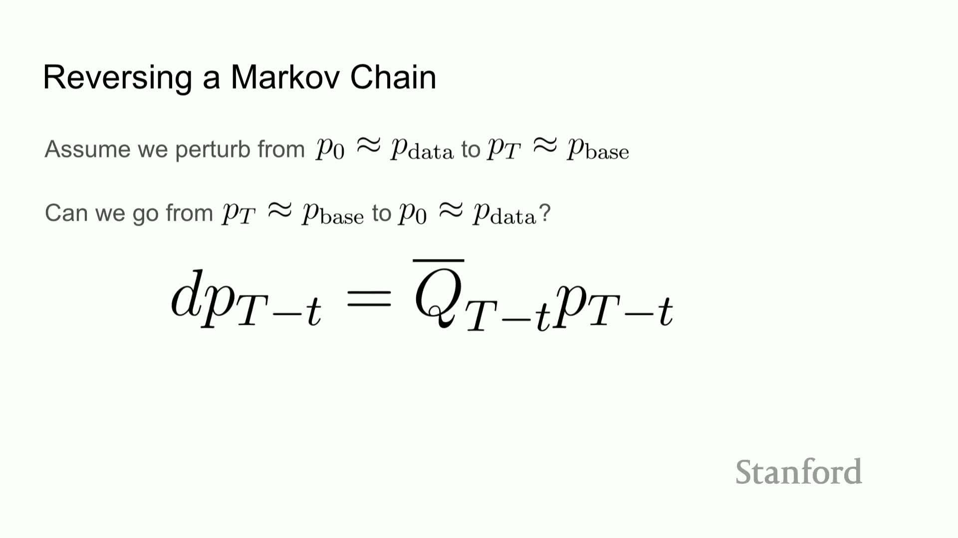
The concrete score must be estimated as a function of noise level or time t to produce ratios for intermediate distributions p_t.
Practical extension:
- Make the model time-conditioned so it predicts local density ratios conditional on the current corruption level, analogous to time-conditioned score networks in continuous diffusion.
- Train with the denoising score-entropy loss applied at multiple t values sampled from a schedule, enabling the network to represent the family of intermediate concrete scores required for reverse sampling.
Reverse diffusion and relation between forward and reverse generators
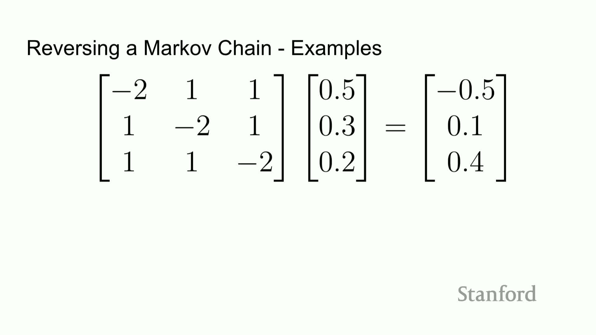
The reverse-time diffusion dynamics are defined by a rate matrix Q̄_t that depends on forward-time rates and the ratios p_t(j)/p_t(i):
- For i ≠ j, Q̄_t(i → j) ∝ Q_t(j → i) * p_t(j) / p_t(i).
- Diagonal entries are set to enforce column sums of zero.
This relationship shows the reverse generator can be written in terms of the forward generator and the concrete score ratios, making it possible to approximate reverse dynamics by substituting learned estimates of the concrete score.
Sampling from the reverse process using the learned concrete score
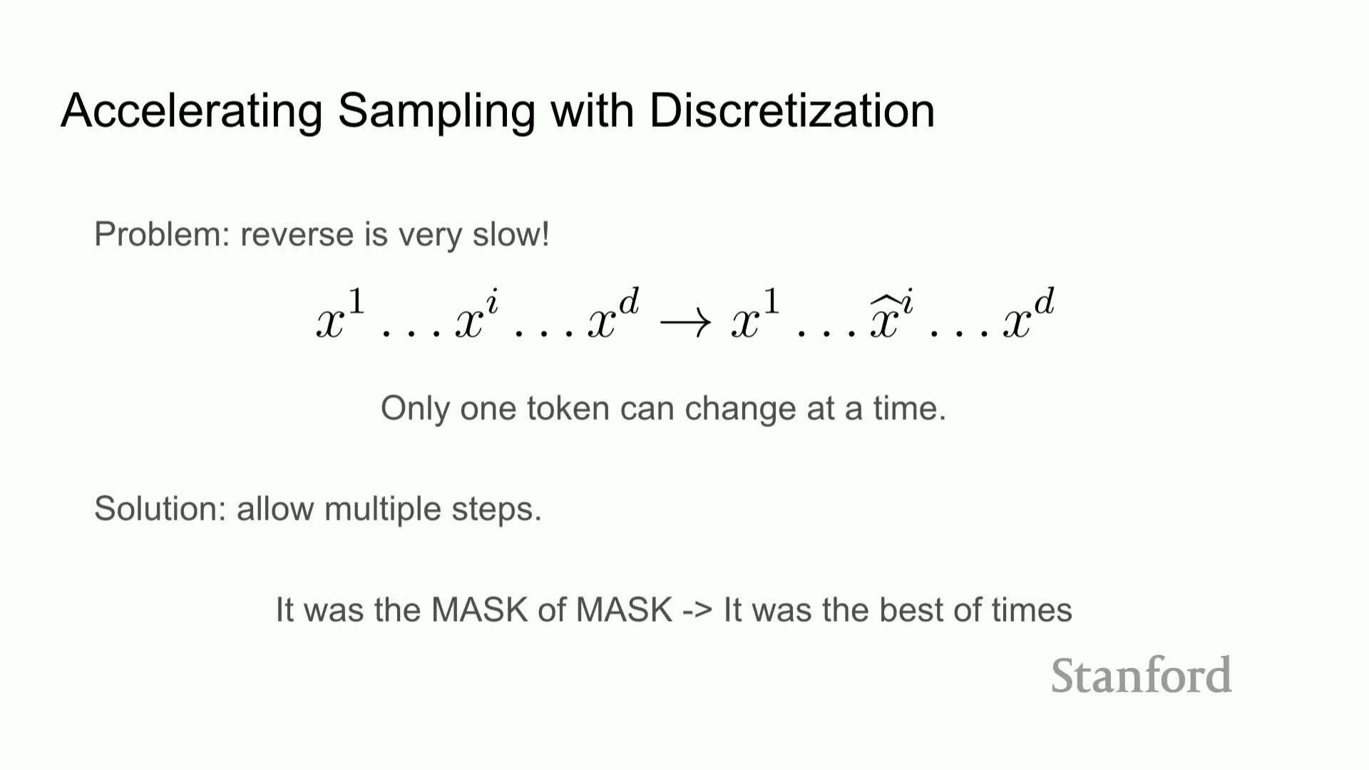
Given the learned time-dependent concrete score network, sampling proceeds by simulating the reverse-time Markov chain:
- Transition probabilities are computed from the estimated ratios and the known forward Q_t.
- The parameterization yields parallel updates across token positions because the model provides per-position conditional ratios, enabling simultaneous proposed jumps to multiple states.
This produces a discrete reverse diffusion sampler analogous to ancestral sampling for continuous diffusion models but driven by estimated local density ratios.
Computational bottleneck of single-token jumping and simultaneous-step acceleration
Exact reverse simulation that flips single tokens per step can be computationally expensive because many small transitions are required to reach a clean sequence.
To accelerate sampling:
- Perform multiple token updates (simultaneous jumps) per reverse step, effectively leapfrogging several single-token transitions in one operation.
- This controlled coarsening is a discretization strategy that trades per-step accuracy for sampling speed, akin to tau-leaping methods in stochastic chemical kinetics.
- Empirical tuning balances speed and sample fidelity.
End-to-end pipeline and illustrative text generation

The complete pipeline:
- Sample data from P_data.
- Define a forward discrete diffusion process (e.g., mask or uniform).
- Train a time-conditioned concrete score network with denoising score-entropy.
- Run the learned reverse chain with multi-step acceleration to generate sequences.
Notes:
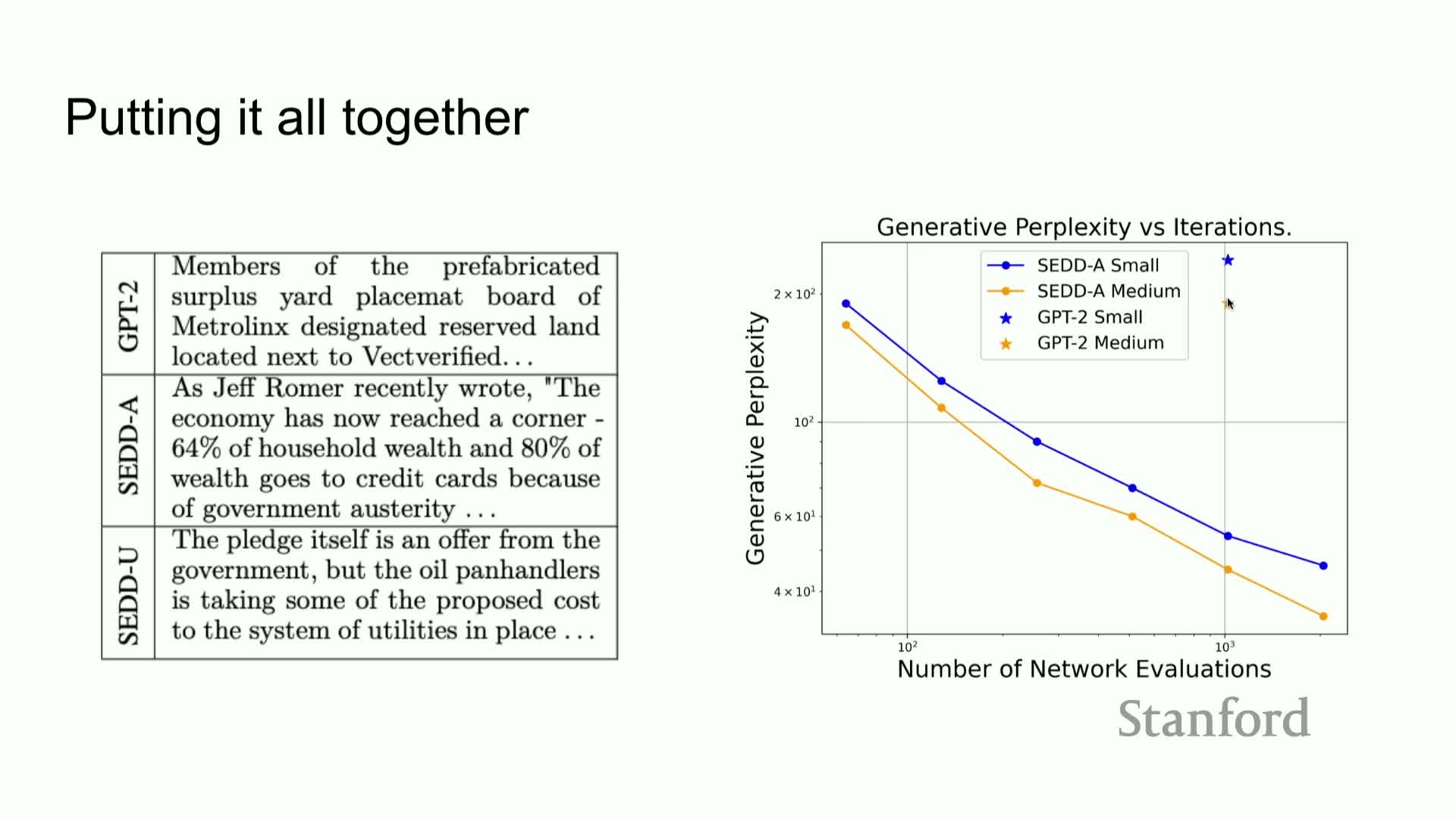
- Example generations using models of GPT-2 scale demonstrate plausible and coherent text outputs, indicating the method can produce high-quality sequences without autoregressive decoding.
- The pipeline is modular: choice of Q, corruption schedule, and sampling discretization together control quality and speed.
Quality-versus-compute trade-off and comparison to autoregressive models
Discrete diffusion models (termed SDD in the lecture) exhibit a trade-off between the number of reverse sampling steps and sample quality:
- Increasing steps yields monotonic improvements in generation quality, often in a log-linear manner.
- At moderate numbers of steps (e.g., ~64) SDD can match autoregressive models like GPT-2 in perceived coherence while offering faster parallel sampling.
- With larger step budgets SDD quality improves further and can surpass small autoregressive baselines.
This demonstrates controllable compute–quality trade-offs that are absent in strictly sequential autoregressive decoders.
Controllable generation and flexible conditioning (prompting and infill)
The discrete diffusion framework supports conditioning on arbitrary token subsets, enabling principled in-filling and arbitrary-location prompting:
- Clamp known tokens and sample the rest under the reverse dynamics.
- Because reverse transitions operate over entire sequences rather than strictly left-to-right, conditioning can be applied at middle or multiple positions and the sampler will generate context-consistent completions around fixed tokens.
This flexibility yields control modalities that are difficult to realize with strictly causal autoregressive decoders.
Likelihood evaluation and a perplexity upper bound via denoising score entropy

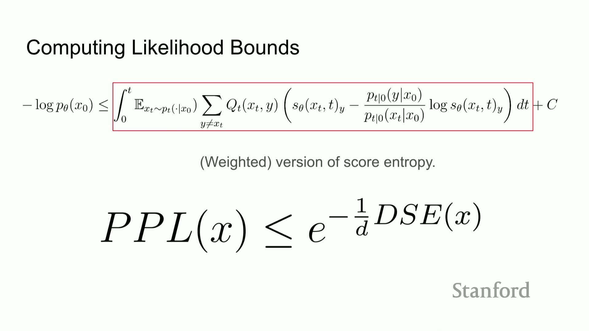
Perplexity, the standard metric for language-model likelihood evaluation, can be upper-bounded for discrete diffusion models by an expected denoising score-entropy functional plus a known constant under mild conditions on the base distribution and diffusion schedule.
Concretely:
- Negative log-likelihood is bounded by an integral of expectations that mirrors the denoising objective used in training.
- This allows reporting perplexity bounds computed from the learned model and corruption kernel, providing a principled comparison to autoregressive likelihoods.
Empirical likelihood and perplexity comparisons to autoregressive baselines
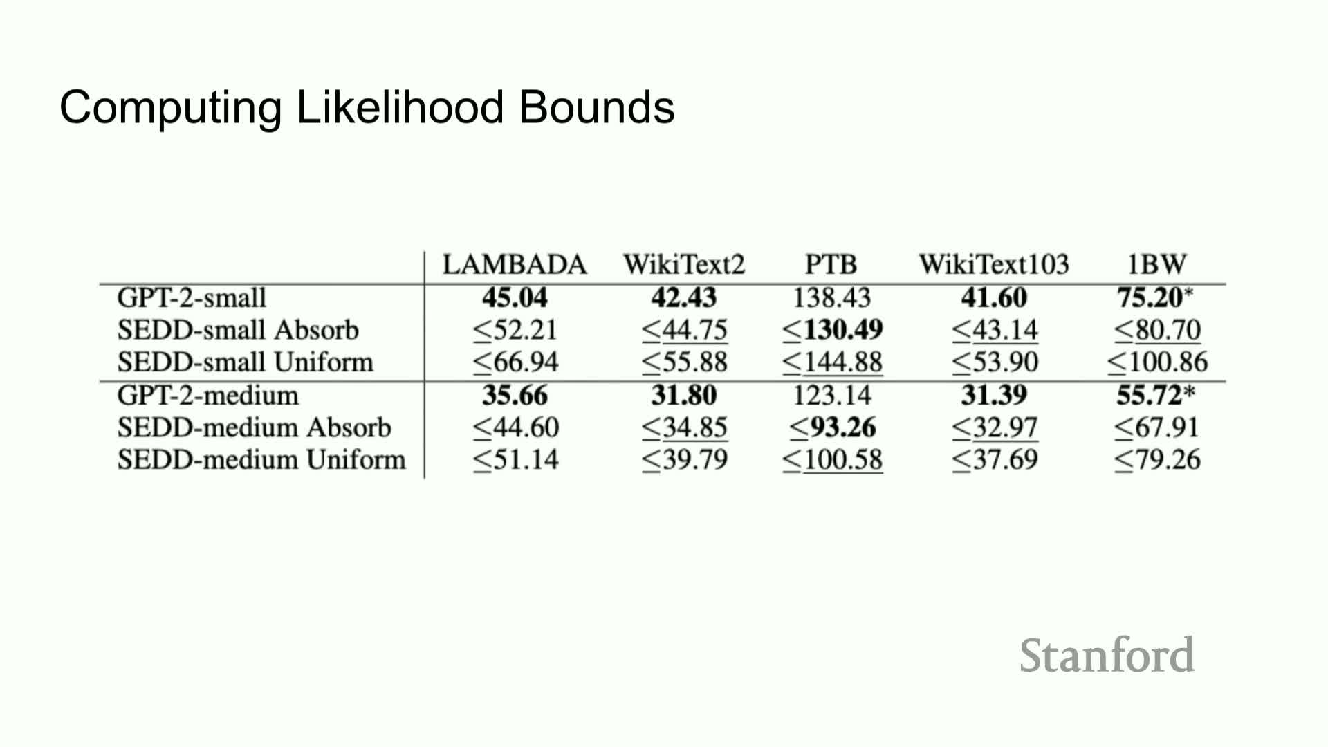
Empirical evaluations show:
- Autoregressive GPT-2 models often achieve the best (lowest) perplexity.
- Discrete diffusion (SDD) models with absorbing-mask transitions frequently achieve comparable perplexities within a modest bound (e.g., within ~10%) and sometimes outperform on certain datasets.
Caveat:
- The reported numbers are upper bounds on negative log-likelihood derived from the denoising objective, so close performance indicates SDD models cover data modes sufficiently well and can be competitive with autoregressive baselines on standard language datasets.
Summary and concluding observations
In summary:
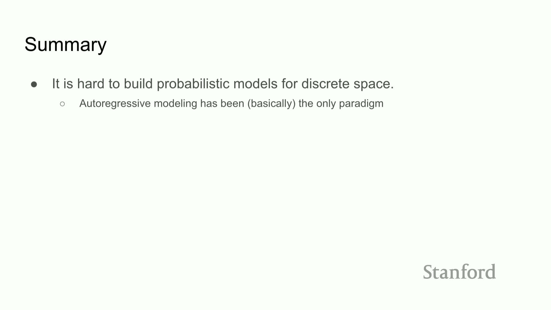
- Continuous generative methods do not directly transfer to sparse token spaces, making discrete probabilistic modeling challenging.
-
Score-based techniques can be generalized by replacing continuous gradients with finite-difference density ratios (the concrete score).
- Training via score-entropy and denoising score-entropy yields tractable objectives; diffusion forward mechanisms (Q matrices) provide principled corruption; and reverse-time sampling driven by learned concrete scores permits parallel and controllable generation.
Empirical results indicate discrete diffusion models can match or surpass autoregressive baselines in generation quality and approach comparable likelihoods, opening an alternative paradigm for discrete sequence modeling.
Enjoy Reading This Article?
Here are some more articles you might like to read next: