CS336 Lecture 2 - PyTorch, resource accounting
- Course objectives and lecture plan
- Napkin-math approach for large-scale training time estimation
- Memory-limited model size estimation on GPUs
- Pedagogical focus on primitives and resource-accounting mindset
- Tensors and floating-point data types: FP32, FP16, BF16, FP8
- Device placement and data movement between CPU and GPU
- Tensor storage model, views, strides, contiguity and mutation semantics
- Matrix multiplication, batching and einsum-style dimension naming
- FLOPs terminology, hardware peak performance and marketing caveats
- Matmul FLOP cost formula and MFU benchmarking
- Gradient computation cost and the six-times rule
- Parameter objects and initialization best practices
- Deterministic seeding and large-scale token data loading
- Optimizers, per-parameter state, and total memory accounting
- Activation storage, checkpointing, training loop, mixed precision and checkpointing
Course objectives and lecture plan
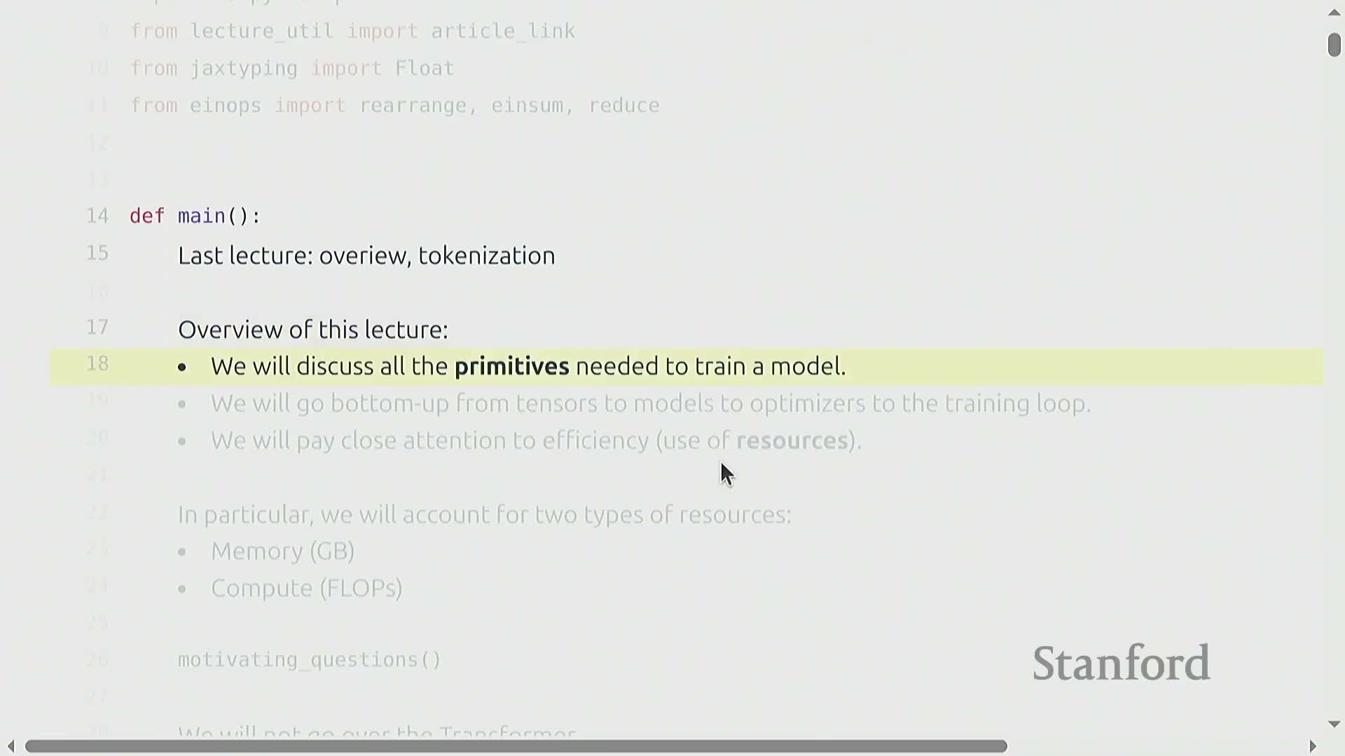
Objective: Demonstrate how to build language models from first principles, emphasizing PyTorch primitives, model construction, optimizers, and an efficient training loop.
The lecture prioritizes practical mechanics over high-level architecture. Key focus areas include:
-
Tensors — representation, manipulation, and lifecycle in training
-
Parameter storage — how model parameters are stored and updated
-
Computation placement — deciding where operations run (CPU vs GPU) and why it matters
-
Resource accounting — precise tracking of memory and compute (FLOPs and bytes) to inform design and scale decisions
Efficiency is treated as a first-class concern: the lecture motivates why exact bookkeeping of FLOPs and bytes matters when scaling models and systems.
Student expectations:
-
Apply these primitives directly in assignments and implementation exercises.
-
Defer architectural deep-dives (for example, the transformer) until those topics are covered later in the course.
Napkin-math approach for large-scale training time estimation
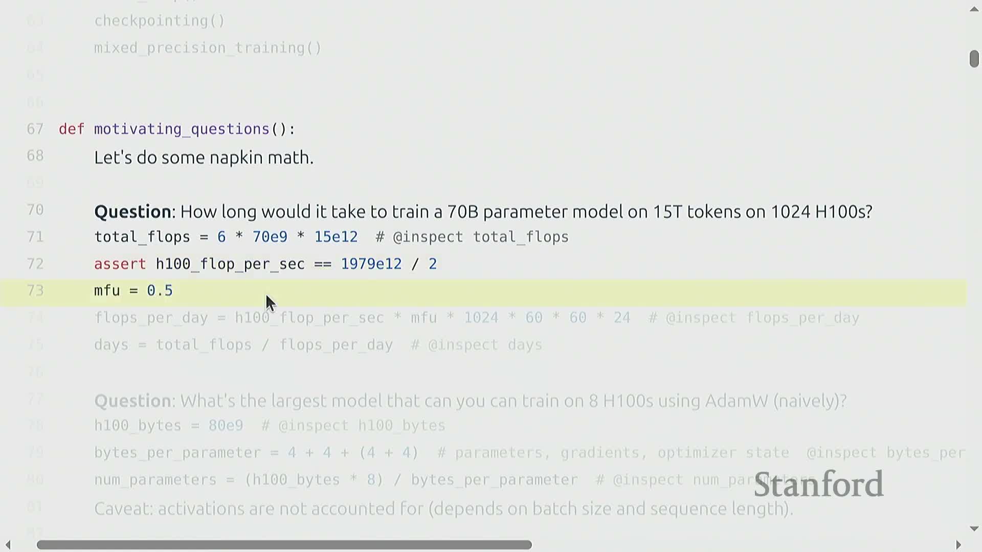
Training-time estimation (order-of-magnitude)
-
Compute total training FLOPs:
- Use the rule of thumb: Total training FLOPs ≈ 6 × number_of_parameters × number_of_tokens.
- The factor of six accounts for forward and backward computation across the training run.
- Use the rule of thumb: Total training FLOPs ≈ 6 × number_of_parameters × number_of_tokens.
-
Compute effective hardware throughput:
-
Effective throughput = hardware peak FLOPs/sec × model FLOPs utilization (MFU).
- A practical choice in this method is MFU = 0.5; combining that with H100 spec-sheet peak FLOPs gives a concrete throughput estimate.
-
Effective throughput = hardware peak FLOPs/sec × model FLOPs utilization (MFU).
-
Estimate training time:
-
Training time ≈ Total training FLOPs / Effective throughput.
-
Training time ≈ Total training FLOPs / Effective throughput.
Notes:
- This approach gives quick, order-of-magnitude answers useful for cost and resource planning for very large models.
- It relies on the simplified 6 × parameters × tokens FLOPs rule and an assumed MFU, so treat results as estimates rather than precise timings.
Memory-limited model size estimation on GPUs
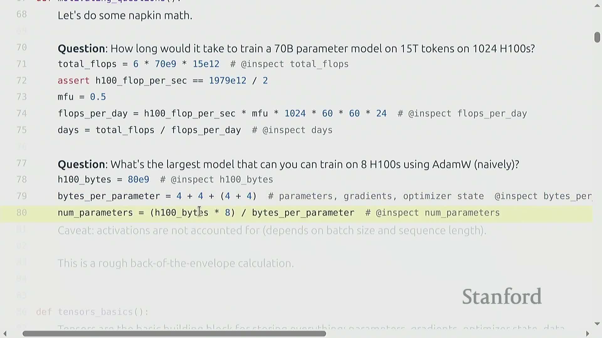
The maximum parameter count that can be stored on a GPU fleet is constrained by high-bandwidth memory (HBM) capacity and the per-parameter byte footprint required for parameters, gradients, and optimizer state.
Example (back-of-the-envelope):
-
Available HBM per device: e.g., an 80 GB HBM device.
-
Per-parameter footprint: roughly 16 bytes per parameter (accounting for parameter values, gradient accumulator, and optimizer state in FP32).
-
Resulting scale: this yields on the order of tens of billions of parameters per device (coarse estimate).
Key caveats:
- The estimate deliberately omits activation storage, which can be significant depending on architecture and training phase.
- The usable parameter capacity also depends on batch and sequence sizes, and on whether additional runtime memory is needed for other tensors or kernels.
Why this matters:
- This coarse calculation is sufficient to scope feasible model sizes.
- It directly informs decisions about model parallelism and precision reduction strategies (e.g., moving to lower-precision formats to reduce per-parameter footprint).
Pedagogical focus on primitives and resource-accounting mindset
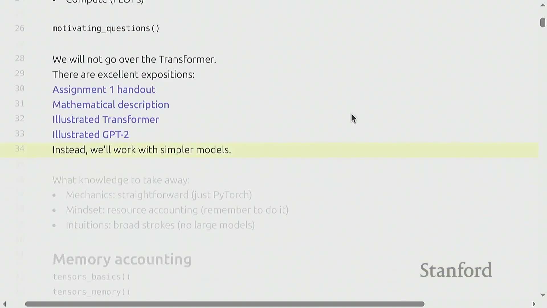
Instructional emphasis is on mastering low-level primitives in PyTorch and developing a resource-accounting mindset, rather than on the architectural theory of transformers.
Practical goals are to:
-
Measure and reason about where memory and compute are used in a model pipeline—identify hotspots and understand per-layer/resource costs.
- Make design choices that explicitly trade off accuracy, numerical stability, and runtime/memory cost—weigh correctness against performance and resource limits.
- Build a foundation for applying resource-aware optimizations when scaling to larger architectures or integrating hardware-aware techniques.
This foundation enables informed, resource-conscious engineering later on, so optimizations are driven by measured costs and clear trade-offs rather than by opaque abstractions.
Tensors and floating-point data types: FP32, FP16, BF16, FP8
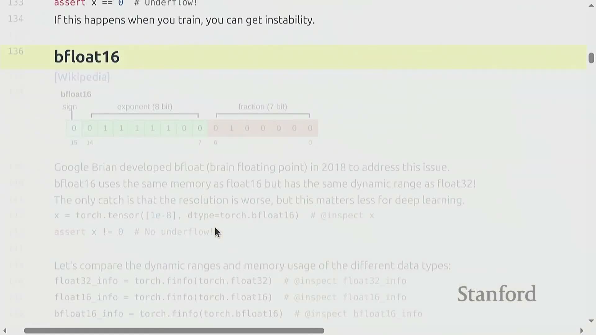
Tensors are the fundamental storage objects. Their memory footprint equals the number of elements × bytes per element, where the bytes per element are determined by the chosen floating‑point format.
-
FP32 (32‑bit) — common baseline; 4 bytes per element.
-
FP16 (16‑bit) — roughly halves memory (≈2 bytes per element) but has reduced dynamic range and can underflow/overflow for very small/large values.
-
BF16 (bfloat16) — keeps FP32 dynamic range while using FP16 memory by reallocating exponent bits; a practical choice for many training computations.
-
FP8 — offers further memory reduction at the cost of precision; requires specialized hardware support and careful numeric handling.
In production training people typically use mixed precision to balance efficiency and stability:
- Use lower precision for transient compute to reduce memory and increase throughput.
- Keep higher precision (FP32) for parameters and optimizer state to preserve numerical stability.
Device placement and data movement between CPU and GPU
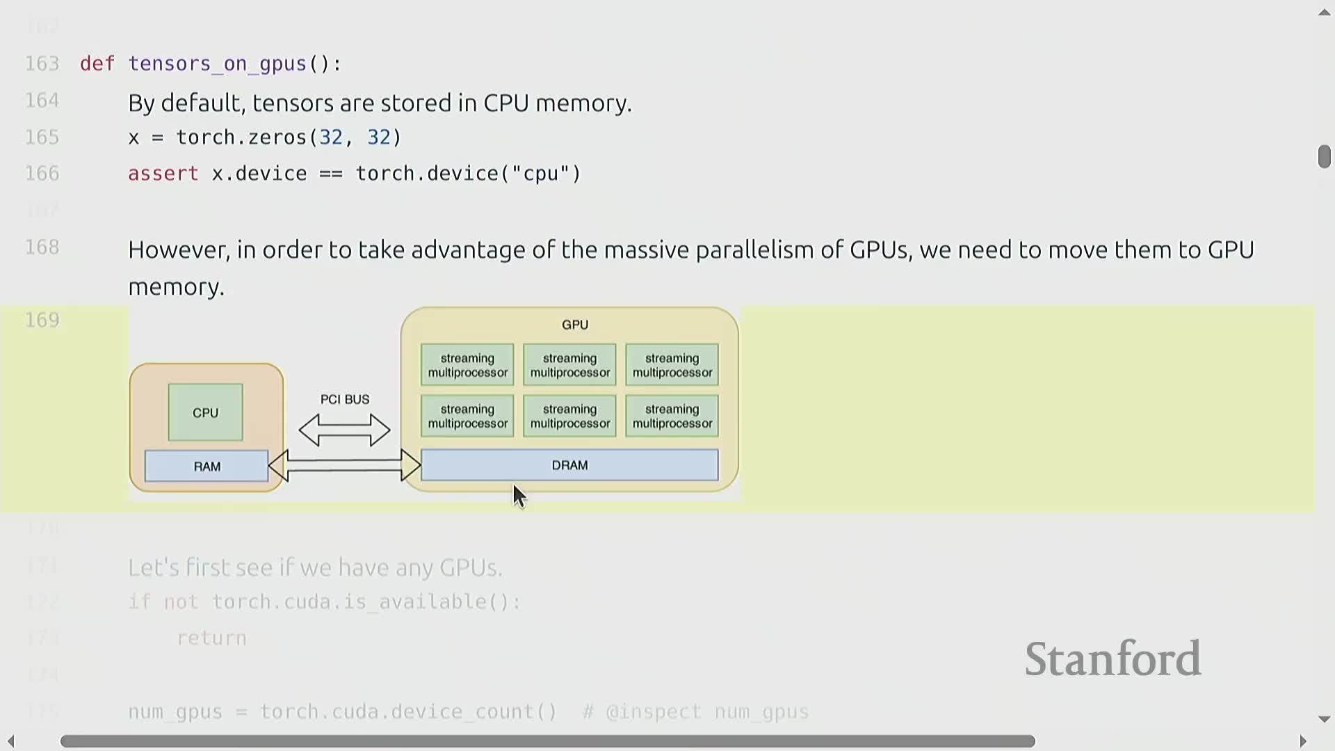
By default, tensors are allocated on the host (CPU) and must be explicitly moved to accelerator devices (GPU) to exploit hardware acceleration — this movement incurs a nontrivial host-to-device transfer cost.
Creating tensors directly on the target device avoids that copy and the associated overhead.
Use instrumentation or asserts in code to track where a tensor resides. This helps prevent accidental transfers and the resulting performance degradation.
Typical workflows to minimize transfer overhead:
-
Allocate model parameters on GPU memory whenever possible so they do not need repeated transfers.
-
Create or move input batches to GPU once per batch, rather than moving individual tensors frequently.
-
Check memory allocated before and after operations as a quick sanity check for unexpected allocations or copies.
-
Design pipelines to minimize frequent host-device round-trips by batching work and keeping data and computation co-located.
Following these practices reduces unnecessary transfers and preserves the performance benefits of accelerators.
Tensor storage model, views, strides, contiguity and mutation semantics
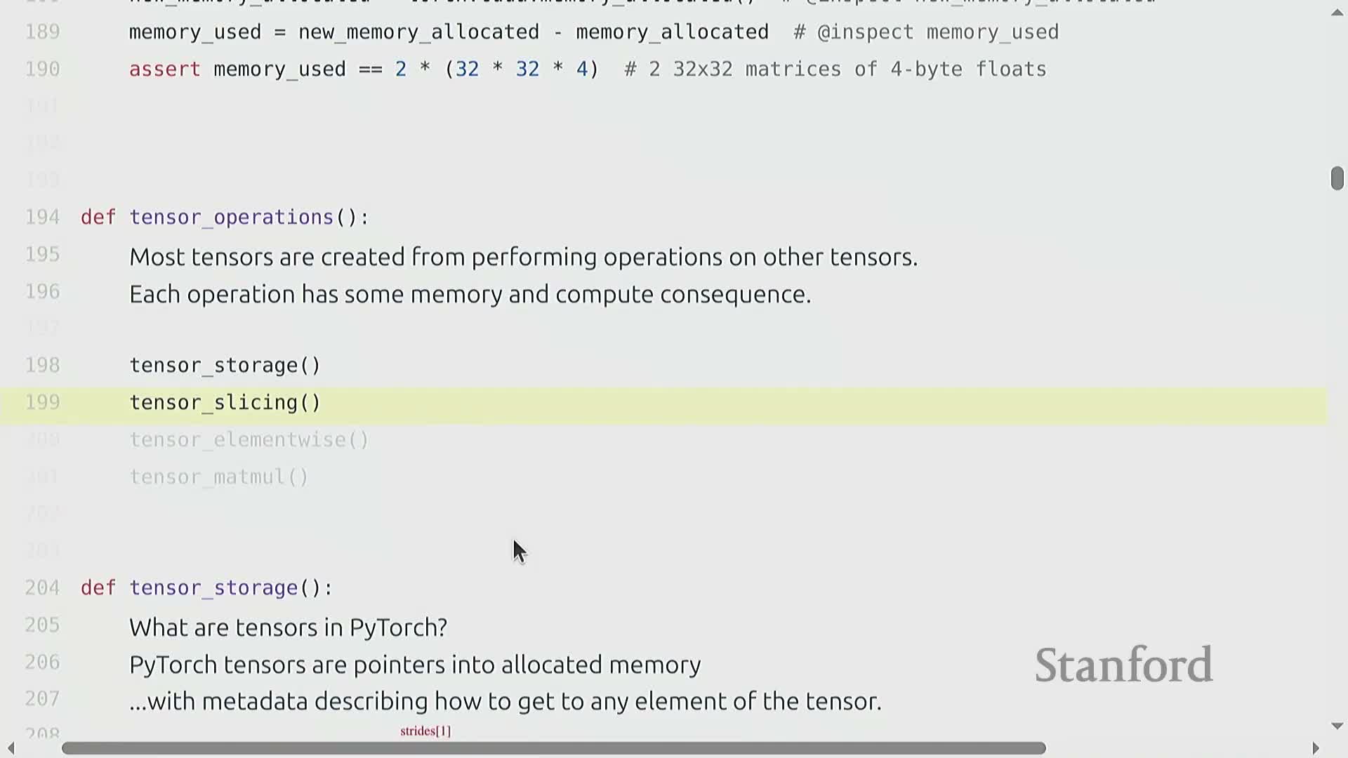
A PyTorch tensor is essentially metadata—its shape and strides—that index into an underlying contiguous storage buffer. The stride for each dimension determines how to compute the storage offset for an index.
- Many tensor manipulations create zero-copy views that share the same storage:
-
slices
-
transposes
-
reshapes (via view)
Mutating one view will therefore mutate the underlying buffer and affect other views that reference it.
-
slices
- Some view operations produce non-contiguous memory layouts. Calling .contiguous() forces replication into a contiguous buffer and thus produces a copy.
Understanding these semantics is essential to control memory use, avoid inadvertent data duplication, and reason about correctness when in-place mutations occur.
Matrix multiplication, batching and einsum-style dimension naming
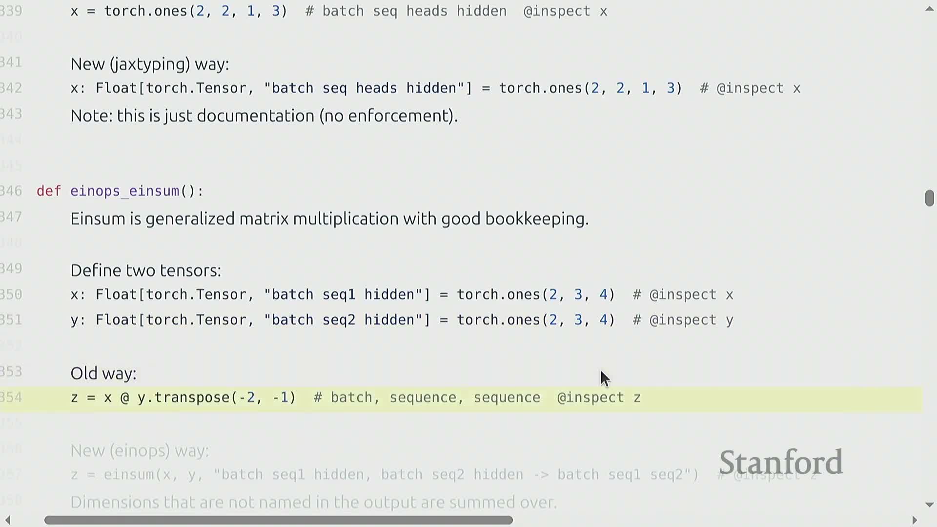
Matrix multiplication is the computational workhorse of deep learning and is typically executed in batched form, where tensors carry batch and sequence dimensions in addition to per-token feature dimensions.
-
Batched matmul semantics: a (B×S×M) tensor multiplied by an (M×K) matrix performs the same M×K matmul for every batch/sequence element, producing a (B×S×K) result.
- This pattern is pervasive in language models and underlies most token-wise linear transformations.
- This pattern is pervasive in language models and underlies most token-wise linear transformations.
Dimension-naming conventions such as einsum or einops/rearrange provide readable, explicit specifications of tensor contractions and reshapes:
- Reduce indexing errors by making intent explicit.
- Can be compiled efficiently into optimized kernels.
- Make multi-head and head-splitting operations (e.g., head × head_dim ↔ flattened hidden_dim) explicit and auditable, simplifying reasoning about model internals.
FLOPs terminology, hardware peak performance and marketing caveats
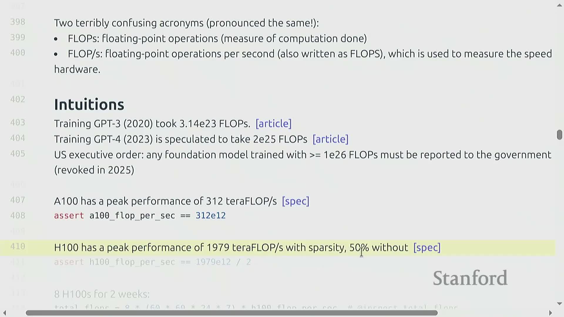
FLOPs = count of floating‑point operations, while FLOPs/sec = floating‑point operations per second, a measure of hardware throughput.
-
Hardware peak FLOPs/sec depends strongly on data type and availability of specialized units (e.g., tensor cores).
-
Vendor specs often quote idealized peaks that assume sparsity or specific data types; these quoted peaks are a useful upper bound but are not a guarantee of real-world performance.
Practical evaluation requires benchmarking real kernels on your target shapes and data types because several implementation factors substantially affect realized performance:
- Measure kernels on the actual shapes and data types you will use — theoretical peaks may not apply.
- Account for memory bandwidth, kernel shape, and runtime overheads (launch, synchronization, packing, etc.), which frequently dominate performance.
- Use vendor peaks only as an upper bound and rely on empirical benchmarks to determine achievable throughput.
Matmul FLOP cost formula and MFU benchmarking
A dense matrix multiplication of shapes (m×n) × (n×p) requires 2 × m × n × p FLOPs — one multiply and one add per inner-product component.
The same rule extends to batched matmuls by applying the calculation per batch/sequence element.
For model-level accounting, the forward pass FLOPs often reduce to approximately 2 × tokens × parameters.
Measuring utilization is a small process:
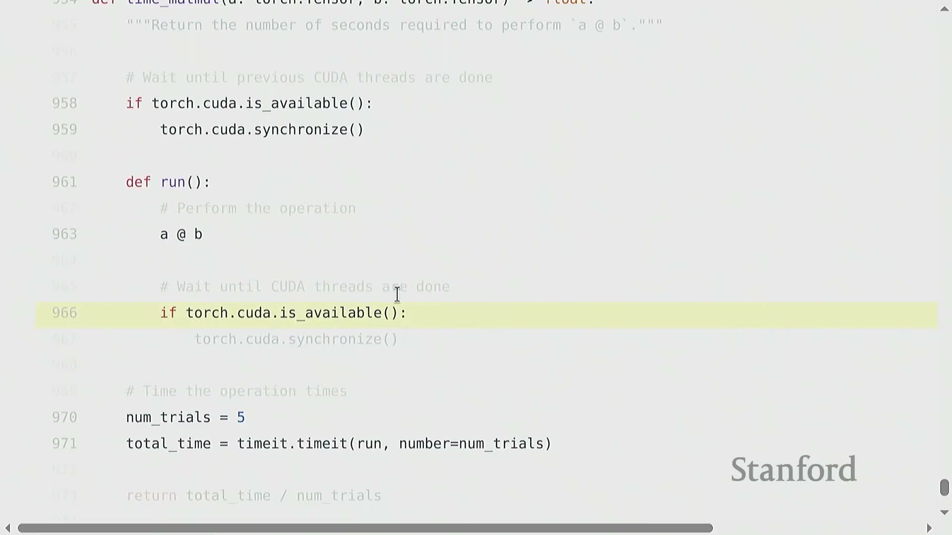
- Time the kernel to get measured FLOPs/sec.
- Divide that by the hardware theoretical peak FLOPs/sec.
- The ratio is Model FLOPs Utilization (MFU) — a practical metric for how effectively the workload uses the hardware.
-
MFU values above ~0.5 are common targets for good utilization.
- Datatype choices (e.g., FP32, BF16, FP8) and the use of tensor cores affect both the peak and measured FLOPs/sec, and thus influence MFU.
Gradient computation cost and the six-times rule
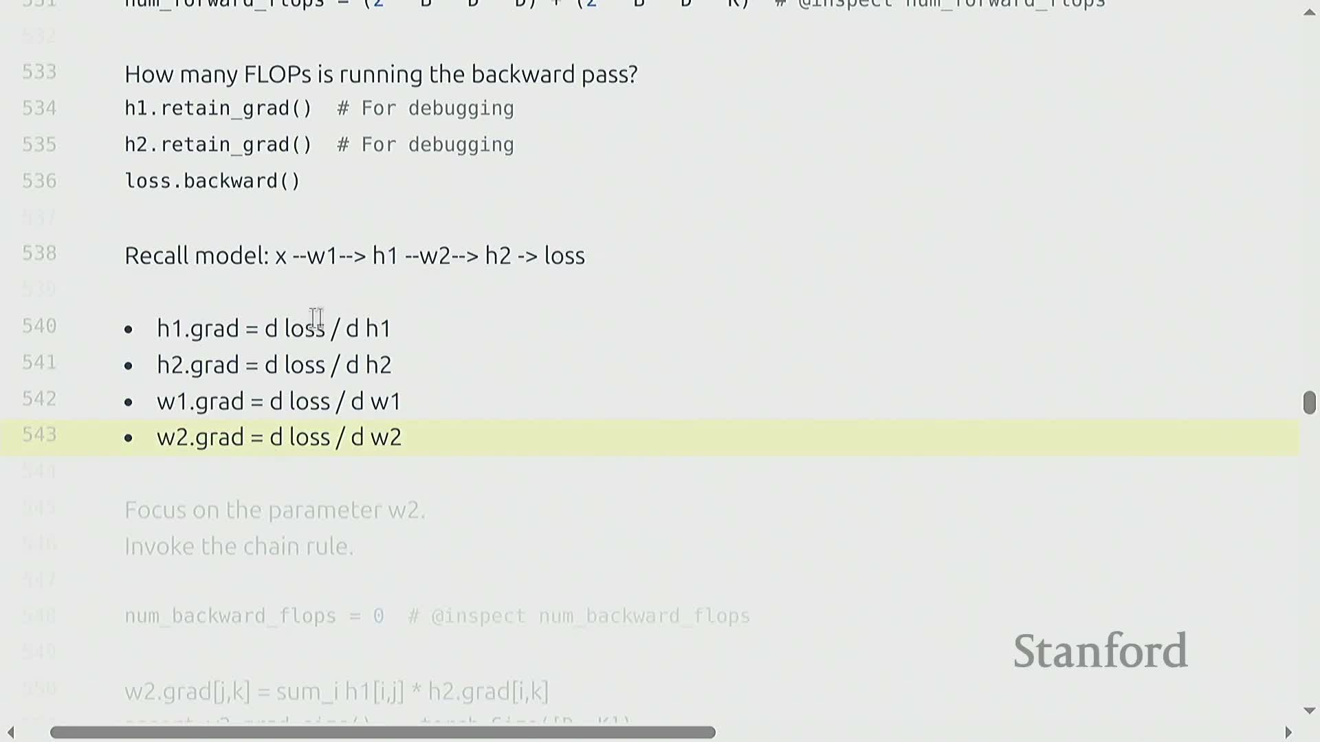
Backpropagation increases compute cost relative to a forward pass because gradients require additional matrix operations whose dimensions mirror those in the forward path.
For typical dense layers, the backward work is about twice the forward work per parameter.
Worked example (linear layers):
-
Forward pass: cost ≈ 2 × tokens × parameters.
-
Backward pass (gradients): cost ≈ 4 × tokens × parameters.
-
Total per training step: ≈ 6 × tokens × parameters — the six-times multiplier.
This six-times multiplier is a practical rule-of-thumb that captures the dominant cost when per-step matrix multiplications touch most parameters, and it’s widely used for napkin-scale training-time estimates.
Parameter objects and initialization best practices
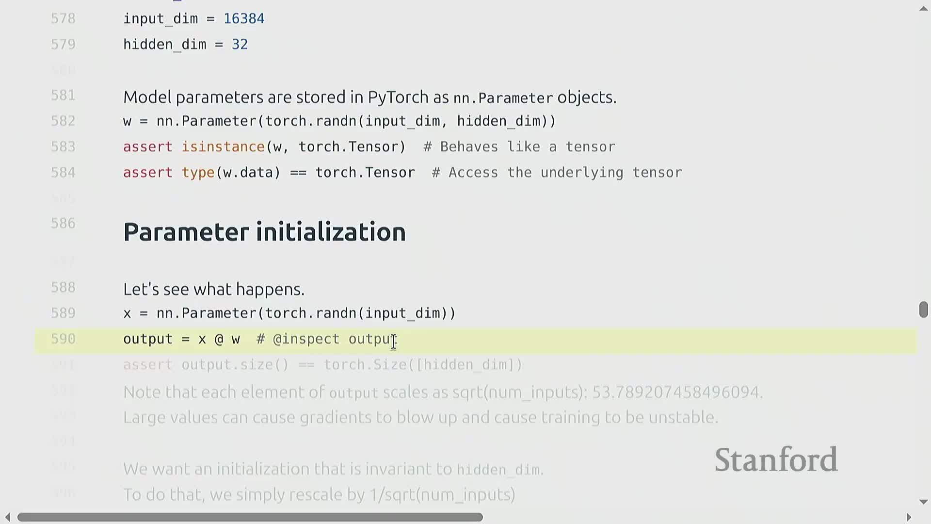
Parameters in PyTorch are represented by nn.Parameter objects and must be initialized to avoid large variance growth across layers.
A naive i.i.d. Gaussian initialization yields activation variances that scale with dimensionality, which can destabilize training as network width or depth increases.
Common remedies and best practices:
- Use Xavier-style (Glorot) scaling — rescale random initial weights by 1/√fan_in (or an equivalent constant) to keep activation magnitudes order-one across layers.
- Consider truncated distributions to limit extreme tail values from the random initializer, reducing outlier weights that harm training stability.
Proper initialization reduces the need for corrective learning-rate hacking and improves numerical stability, particularly for deep or wide linear blocks.
Deterministic seeding and large-scale token data loading
Reproducibility requires deterministic handling of all randomness sources, including:
-
parameter initialization
-
data ordering
-
augmentation
Setting distinct, fixed seeds per randomness source enables targeted experiments and simplifies debugging.
Tokenized language datasets are sequences of integers and can be extremely large (often terabytes).
Use memory-mapped file access (e.g., numpy.memmap) to expose on-disk data as array-like objects without loading full datasets into RAM.
- This provides efficient, low-memory access to very large token sequences
- Keeps the dataset accessible via familiar NumPy-style indexing and slicing
To train from memmap-backed data, follow a simple workflow:
- Create a numpy.memmap that points to the tokenized on-disk file.
- Use a DataLoader-style sampler to draw indices or ranges from the memmap.
- Form minibatches by indexing the memmap with those indices and feed them to the training loop.
This yields training batches while keeping memory usage bounded and predictable.
Optimizers, per-parameter state, and total memory accounting
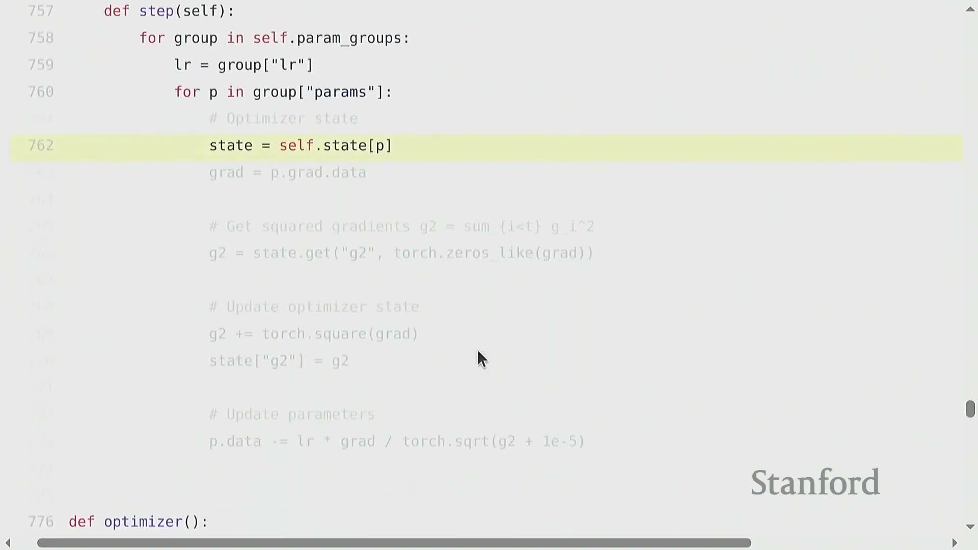
Optimizers maintain per-parameter auxiliary state (e.g., momentum buffers, running averages of squared gradients) that scale with parameter count and must be included in memory budgets.
Classic optimizers and their per-parameter state include:
- SGD with momentum — per-parameter momentum buffer (velocity)
- Adagrad — per-parameter cumulative squared gradients
- RMSProp — per-parameter exponential average of squared gradients
-
Adam — per-parameter first and second moment estimates (mean and squared-mean)
Each algorithm therefore dictates a specific per-parameter state layout and corresponding update rule, which determines how much extra memory the optimizer requires.
Implementations typically maintain a state dictionary keyed by parameter handles, so optimizer state is explicitly associated with each parameter.
Aggregate memory requirement (bytes) can be expressed as:
bytes_per_element × (num_parameters + num_gradients + num_optimizer_states + num_activations)
Where the terms are:
- num_parameters — model weights
- num_gradients — gradient tensors (often same size as parameters)
- num_optimizer_states — additional per-parameter buffers required by the optimizer (varies by algorithm)
-
num_activations — intermediate activations (depends on batch size and architecture)
Because optimizer states scale with parameter count, total memory accounting is essential when sizing models for a given device.
Activation storage, checkpointing, training loop, mixed precision and checkpointing
By default, activations from the forward pass are retained to compute gradients in the backward pass—storing these activations can often dominate memory use.
Activation checkpointing trades extra compute for lower memory by recomputing intermediate activations on demand rather than storing them permanently.
A typical training loop follows these steps:
-
Load batch
-
Forward pass (compute activations and predictions)
-
Compute loss
-
backward() (accumulate gradients using retained/recomputed activations)
-
optimizer.step() (update parameters)
-
Periodically checkpoint the model state, optimizer state, and iteration count to disk to protect long-running training progress
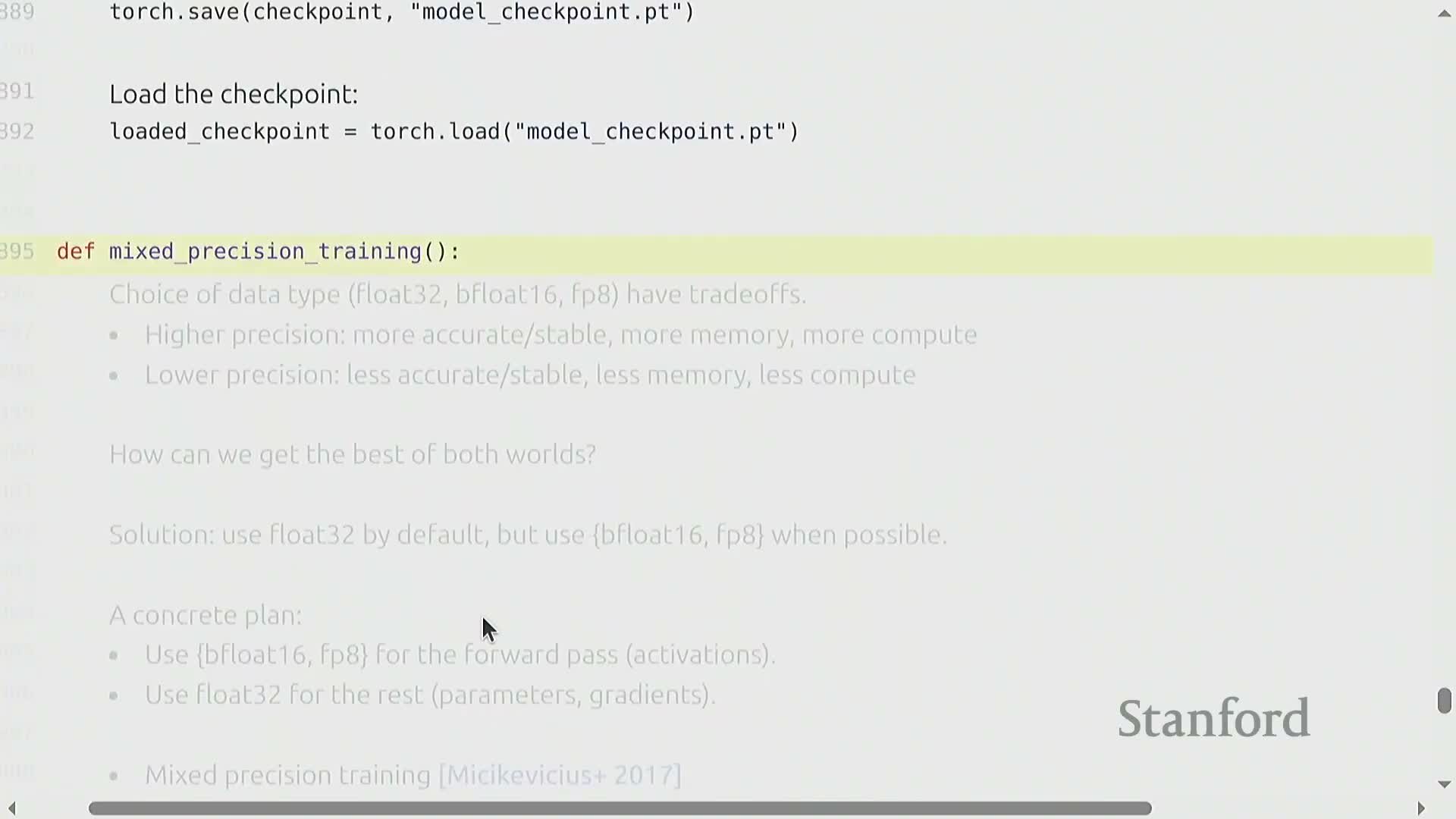
Mixed precision training uses lower-precision formats for transient computation while keeping critical state in higher precision to balance speed and numeric stability:
- Transient compute formats: BF16, FP16, FP8
- Persistent state kept in FP32: parameters, optimizer state
Finally, aggressive post-training quantization can be applied for inference to obtain additional efficiency gains (reduced memory, lower latency, and smaller model size).
Enjoy Reading This Article?
Here are some more articles you might like to read next: