CS336 Lecture 3 - Architectures, hyperparameters
- Lecture overview and objectives
- Recap of the original transformer components
- Survey of recent model releases reveals convergent innovations
- Lecture structure: architecture, hyperparameters, stability and attention variants
- Pre-norm (prenorm) versus post-norm placement of layer normalization
- Double-layer-normalization variants (front and after) as a stability enhancement
- LayerNorm definition and the adoption of RMSNorm for efficiency
- Removing bias terms in linear layers for optimization stability and simplicity
- Generalizable lessons from architectural choices
- Nomenclature and benefits of gated linear units (GLUs) in MLPs
- Gating mechanics and sizing conventions for GLU-based MLPs
- Empirical evidence favors GLU variants but they are not mandatory
- Serial (attention then MLP) versus parallel layer ordering
- Relative positional encodings and RoPE (Rotary Position Embeddings)
- Feed-forward inner dimension (Dff) rule-of-thumb and GLU adjustments
- Attention head sizing and the 1:1 per-head dimension convention
- Aspect ratio (depth versus width) defaults and empirical optima
- Vocabulary sizing trends and multilingual tokenizers
- Dropout, weight decay, and the role of regularization in pretraining
- Consensus hyperparameter defaults as practical starting points
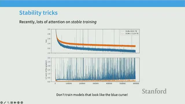
- Training stability issues concentrate around softmax operations
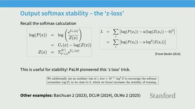
- Z-loss as an auxiliary regularizer for the output softmax
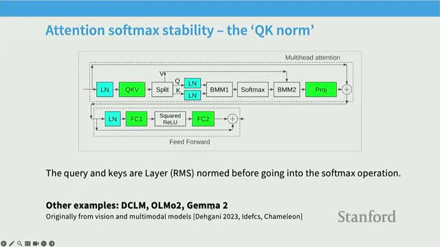
- QK normalization (layer-norm on queries and keys) to tame attention softmax inputs
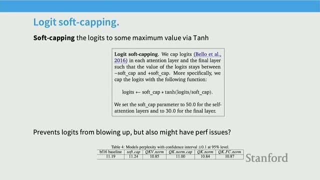
- Soft-capping logits as an alternative clipping strategy
- Inference arithmetic intensity and the motivation for multi-query/group-query attention
- KV cache mechanics and quantitative impact on inference memory and compute
- Sparse, sliding-window, and hybrid attention patterns for long context
Lecture overview and objectives

The lecture introduces architecture and training details for language models and frames the session as an empirical, data-driven examination of transformer variants and hyperparameter choices.
It covers logistics about slides and assignments while positioning the lecture as complementary to hands-on experience by synthesizing common practices across many published models.
Goals and emphasis:
- Identify recurring, practically important architectural and optimization decisions that influence stability, compute efficiency, and final model performance.
- Use empirical patterns to guide defaults and experimental directions.
This framing guides subsequent sections on architecture variations, hyperparameters, and stability tricks.
Recap of the original transformer components
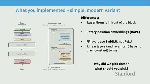
The canonical transformer architecture is composed of several modular components:
-
Input embeddings augmented with positional information.
-
Multi-head self-attention for context-dependent mixing.
-
Residual connections that preserve identity-like signal paths.
-
Layer normalization to control activation scale.
-
Feed-forward MLPs (two-layer position-wise networks).
- A final softmax output that produces probabilistic outputs over vocabulary tokens.
Operationally, each block:
- Processes a residual stream.
- Applies attention and a feed-forward network with interleaved normalization and residual addition.
- Emits logits that the softmax turns into token probabilities.
This componentization creates multiple axes for modification—e.g., layer-norm placement, positional encoding schemes, activation functions, and linear-layer parameterizations—each affecting optimization behavior and runtime.
The remainder of the lecture examines these component variants and their empirical consequences.
Survey of recent model releases reveals convergent innovations

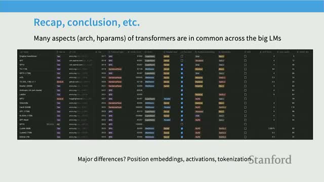
A review of dense model releases (2017–2025) reveals many small, frequent architectural tweaks that nonetheless show convergent evolution in successful designs.
Key observations:
- Tracking axes such as positional encodings, normalization, activation functions, and MLP parameterization yields empirical patterns that inform practical defaults.
- The analysis distinguishes idiosyncratic experiments from consensus choices, enabling practitioners to adopt stable defaults and target experiments where they matter most.
- A spreadsheet-style comparative analysis underpins the lecture’s recommendations, giving concrete evidence for recurring design decisions.
Lecture structure: architecture, hyperparameters, stability and attention variants
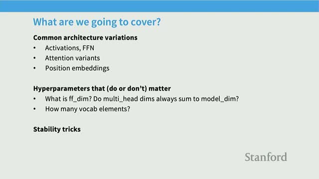
The lecture is organized into three primary sections to match the practical workflow of model design and training:
-
Architecture variations — activations, feed-forwards, attention variants, and positional encodings.
-
Hyperparameter selection — dimensions, MLP ratios, vocabulary sizes, and related choices.
-
Stability interventions — techniques that facilitate large-scale training and reliable convergence.
This roadmap sets expectations for technical depth and empirical emphasis, and signals potential extra coverage of attention variants if time permits.
The organization mirrors practice: choose an architecture, select hyperparameters, then adopt stability and systems-aware practices for training and inference. Each section builds on empirical findings from prior model releases.
Pre-norm (prenorm) versus post-norm placement of layer normalization
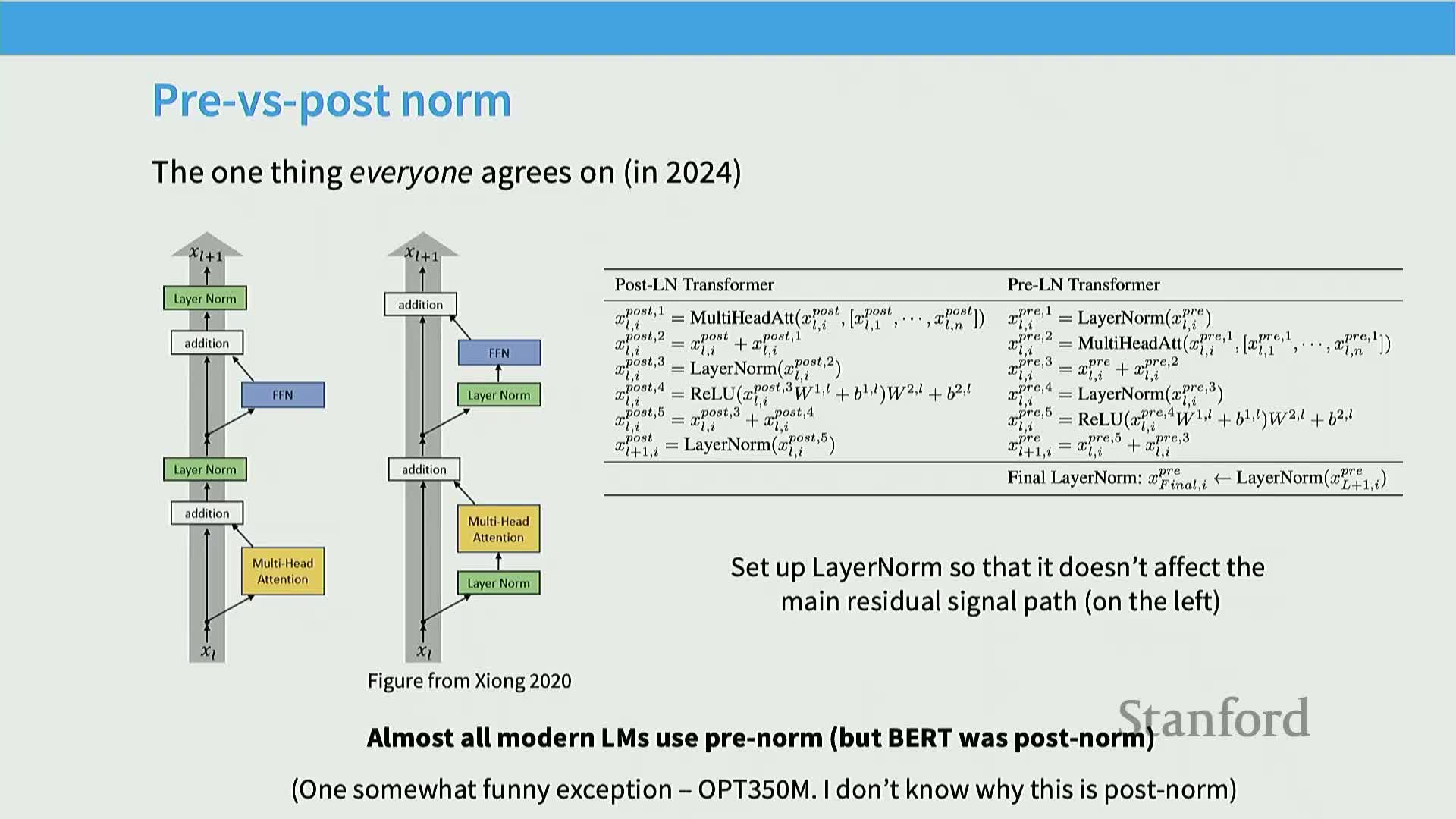
Layer normalization placement substantially affects training stability.
-
Prenorm (normalizing before the sub-block) is empirically far more stable than the original postnorm (normalize after residual addition).
- Benefits of prenorm:
- Reduces loss spikes and gradient explosions during early training.
- Often enables removal of delicate warm-up schedules.
- Improves gradient propagation across many layers, making deep models easier to optimize.
- Reduces loss spikes and gradient explosions during early training.
- Comparisons across translation and BERT-style training show prenorm enables stable optimization for large models without the careful tuning postnorm requires.
Consequently, almost all modern large language model implementations adopt prenorm or prenorm-derived schemes for robustness.
Double-layer-normalization variants (front and after) as a stability enhancement
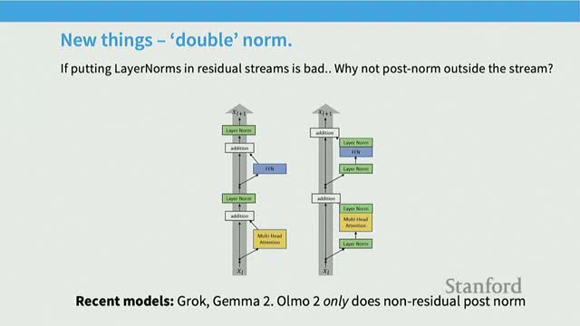
Some recent models add layer normalization both before and after subcomponents (a double-norm) to further improve stability in very large models.
- Pattern: place a normalization at the start of the non-residual computation and again after the block output.
- Empirical effects:
- Further reduces gradient spikes and improves numerical behavior during long or large-scale runs.
- Retains the identity-like property of residual connections while controlling activation scale both entering and exiting sublayers.
- Further reduces gradient spikes and improves numerical behavior during long or large-scale runs.
- Practical note: double-norm adoption is increasing where marginal stability gains matter at scale (e.g., state-of-the-art, extremely deep or high-capacity models).
LayerNorm definition and the adoption of RMSNorm for efficiency
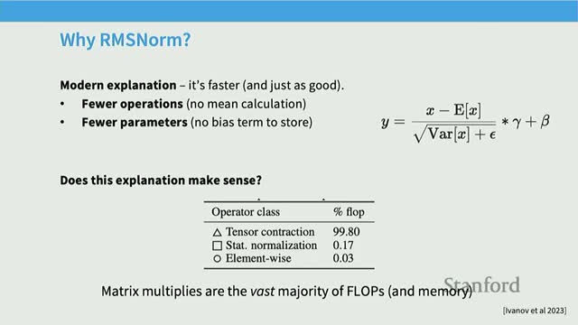
Layer normalization standardizes activations by subtracting the mean and dividing by the standard deviation, then applying learned scale and shift parameters.
RMSNorm is a lighter-weight alternative:
- Removes mean subtraction and the learned bias, scaling only by the root-mean-square (RMS).
- Reduces operations and memory traffic compared to full layer norm.
Systems and empirical trade-offs:
- Normalization ops are negligible in FLOPs but can dominate runtime due to memory movement.
-
RMSNorm reduces parameter loads and runtime overhead while often delivering equivalent model quality.
- Empirical ablations show modest throughput gains and comparable or better final loss with RMSNorm, which is why many modern families (e.g., LLaMA variants, PaLM) converge to RMSNorm.
Choice trade: trivial extra computation versus reduced memory movement and simpler GPU kernels.
Removing bias terms in linear layers for optimization stability and simplicity
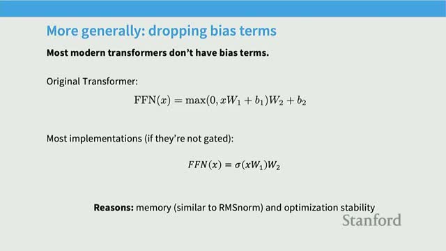
Many contemporary implementations omit bias vectors in linear projections, keeping only pure matrix multiplies to reduce memory movement and simplify numerical behavior.
Practical observations:
- Dropping biases often has no negative effect on final performance and can improve training stability for very large models.
- Possible rationale: avoids small additive perturbations that interact poorly with high learning rates and normalization dynamics.
- Systems benefits: fewer parameters to fetch/update and better opportunity for fused kernels, improving efficiency.
Exceptions: biases may still appear in gated or specially parameterized layers where they have a functional role.
Generalizable lessons from architectural choices

Several architectural rules generalize across model families and scales:
- Prefer identity-preserving residual connections to maintain signal flow.
-
Normalize activations to control scale (via prenorm or RMSNorm).
- Favor gating mechanisms in MLPs for additional representational flexibility (e.g., GLUs).
Why these rules matter:
- They reduce optimization fragility and improve training dynamics as models and datasets scale.
- They interact with system constraints such as memory movement and kernel fusion.
Caveat: these are empirical best practices, not theoretical absolutes—deviations are possible but should be justified experimentally.
Nomenclature and benefits of gated linear units (GLUs) in MLPs
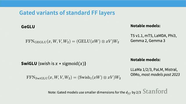
Gated linear units (GLUs) augment the standard two-layer MLP by gating the activation entry-wise with an additional linear projection.
- Mechanism: multiply the primary nonlinearity by a learned gate vector, introducing element-wise multiplicative interactions inside the MLP.
- Benefits:
- Increased representational capacity.
- Conditional computation per hidden dimension.
- Increased representational capacity.
- Variants include GeLU+GLU, SwiGLU (swish-based), and similar gated formulations.
- Empirical outcome: GLUs systematically reduce training loss and improve downstream metrics in many ablation studies.
Practical convention: when using GLUs, reduce the nominal feed-forward hidden size to preserve parameter budgets—commonly scale the hidden dimension so total parameters remain comparable to non-gated baselines.
Gating mechanics and sizing conventions for GLU-based MLPs
How a GLU-based MLP is computed and how practitioners match parameters:
- The input undergoes two linear projections:
- One projection produces the pre-activation passed through a nonlinearity (e.g., GeLU, Swish).
- The other produces a gate vector that modulates the activation element-wise.
- One projection produces the pre-activation passed through a nonlinearity (e.g., GeLU, Swish).
- The gate projection adds parameters and FLOPs, so common practice is to adjust projection sizes to match a non-gated baseline.
Parameter-matching convention:
- Starting from a typical 4× up-projection baseline (Dff ≈ 4 × Dmodel), practitioners set the GLU up-projection so the overall parameter count is comparable.
- A widely used convention reduces the up-projection to about 8/3 × Dmodel, which preserves capacity while capturing gating benefits (roughly an 8/3 factor when starting from a 4× baseline).
Implementation note: ensure the overall parameter budget and memory footprint align with infrastructure constraints when adopting GLUs.
Empirical evidence favors GLU variants but they are not mandatory
Empirical evidence for GLUs:
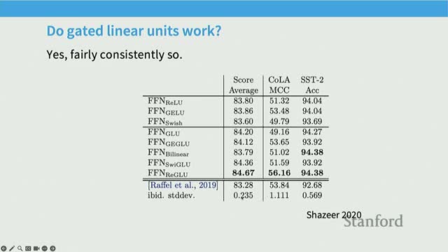
- Multiple ablation studies and benchmarks report consistent gains for GLU-style MLPs (SwiGLU, GeGLU, etc.) over plain ReLU or GeLU on pretraining loss curves and downstream tasks (e.g., GLUE, SST-2).
- These reported improvements have driven broad adoption across post-2023 model releases.
- Counterpoint: several high-performance models (e.g., early GPT-3 variants, some Falcon and Neotron models) succeed without GLUs, showing gating improves but is not strictly necessary.
Practical guidance: treat GLUs as a well-validated improvement to try by default, but evaluate empirical trade-offs given your compute and dataset regime.
Serial (attention then MLP) versus parallel layer ordering
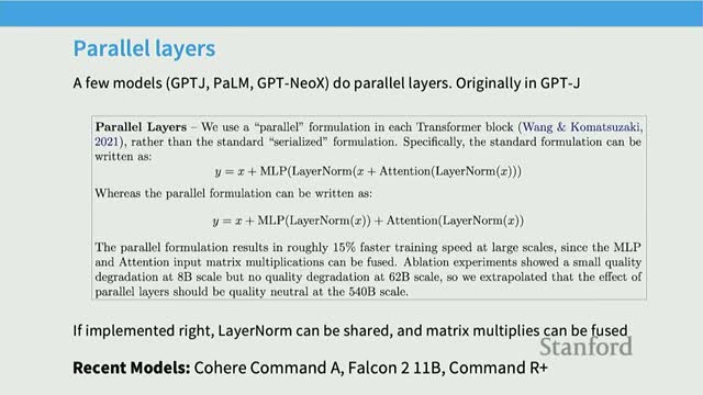
Implementation order in transformer blocks—serial vs parallel architectures:
-
Serial (canonical): attention followed by MLP; intermediate representations are consumed sequentially.
-
Parallel: compute attention and MLP outputs in parallel from the same input and merge them into the residual stream.
Trade-offs:
- Parallelization enables kernel fusion and can better utilize hardware by sharing linear projection computation, potentially improving systems efficiency and reducing per-token latency.
- It changes the computation graph and may alter expressivity compared to serial composition.
- Adoption: explored in models such as GPT-J and PaLM, but most recent models remain serial unless system-level gains justify the change.
Relative positional encodings and RoPE (Rotary Position Embeddings)
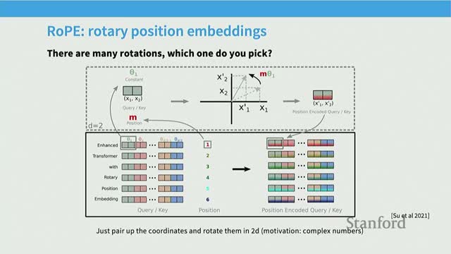
RoPE (Rotary Positional Encoding) encodes position by rotating pairs of vector dimensions by an angle proportional to position.
Key points:
- Splits the model’s D-dimensional vectors into 2D blocks and applies 2×2 rotation matrices parameterized by a schedule of angles.
- Inner products between token embeddings depend only on relative position differences, not absolute positions, realizing a principled relative-position mechanism.
- Applied to queries and keys at the attention layer (not added to base embeddings).
- Empirical benefits: better context-length extrapolation behavior and strong performance even at small scales, leading to widespread adoption.
Feed-forward inner dimension (Dff) rule-of-thumb and GLU adjustments
Feed-forward dimensionality conventions and practical ranges:
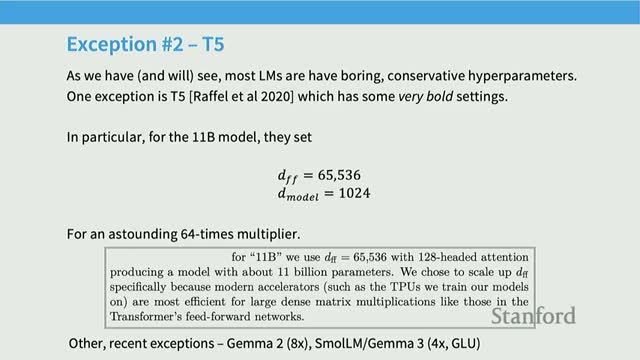
- For conventional (non-gated) MLPs, a standard choice is Dff ≈ 4× Dmodel, balancing expressiveness and compute.
- For GLU-style MLPs, practitioners commonly reduce nominal Dff so parameter counts remain comparable; a widely used convention is Dff ≈ 8/3 × Dmodel.
- Large deviations are possible (e.g., T5’s historical 64× up-projection).
- Empirical scaling-law studies show a broad basin of acceptable ratios (roughly 1×–10×), with modest loss differences, validating the 4× default as a safe starting point.
When changing Dff substantially, consider systems effects (matrix shapes, parallelism) and re-evaluate optimizer and learning-rate schedules.
Attention head sizing and the 1:1 per-head dimension convention
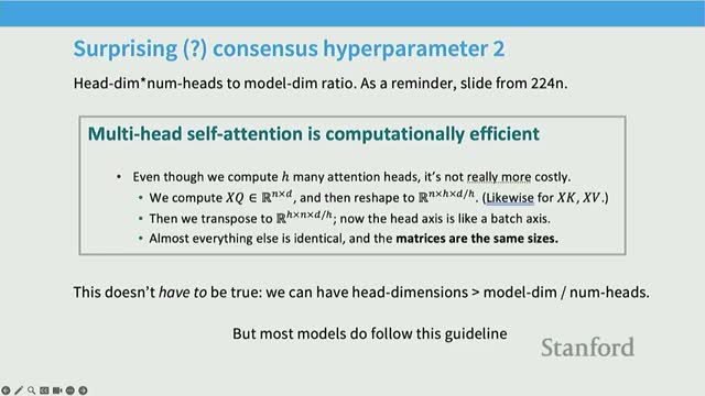
Attention head sizing and the common split convention:
- Most large models split the model hidden dimension D evenly across H heads so each head has dimension D/H, keeping H*(D/H) = D.
- This 1:1-style convention maintains a stable parameterization and computational profile as head count varies and is widely used (GPT-3, PaLM, LLaMA, etc.).
- Theoretical concerns exist that very small per-head dimensions can reduce expressivity (low-rank attention), but in practice the standard split performs well across a wide range of head counts.
Deviations are possible, but any departure from the proportional scheme should be validated empirically for low-rank bottlenecks.
Aspect ratio (depth versus width) defaults and empirical optima
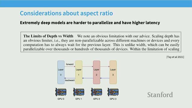
Depth versus width trade-offs and aspect ratios:
- The trade-off is often summarized by aspect ratio metrics (layers vs hidden dimension).
- Empirical studies show a typical optimal band rather than a monotonic preference for deeper or wider networks.
- Practical rule-of-thumb: aim for roughly 128 hidden dimensions per layer at some operating points, though this depends on target model size and infrastructure parallelism.
- Aspect ratio choices interact with system-parallelism strategies (pipeline, tensor parallelism) and can affect downstream fine-tuning behavior.
Recommendation: select aspect ratios that fit hardware constraints and lie within empirically validated basins of good loss; task-dependent experiments may shift the optimum.
Vocabulary sizing trends and multilingual tokenizers
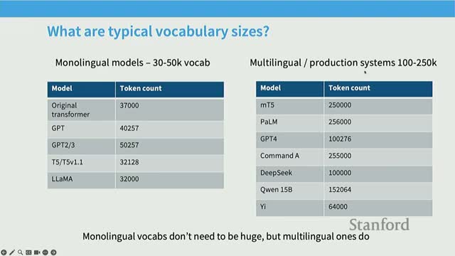
Vocabulary size trends and trade-offs:
- Vocabulary sizes have trended upward from 30k–50k (monolingual) toward 100k–250k for multilingual/production models.
- Larger vocabularies reduce tokenization fragmentation for non-English languages and rare symbols, lowering per-inference token counts and improving user-facing latency and token-cost for multilingual deployments.
- For high-resource languages like English, smaller vocabularies can still be effective, but production models often prioritize larger token sets to reduce tail-mode inefficiencies across many languages.
Choosing vocabulary size balances tokenizer granularity, model parameterization, and downstream inference cost, and should reflect deployment linguistic diversity.
Dropout, weight decay, and the role of regularization in pretraining
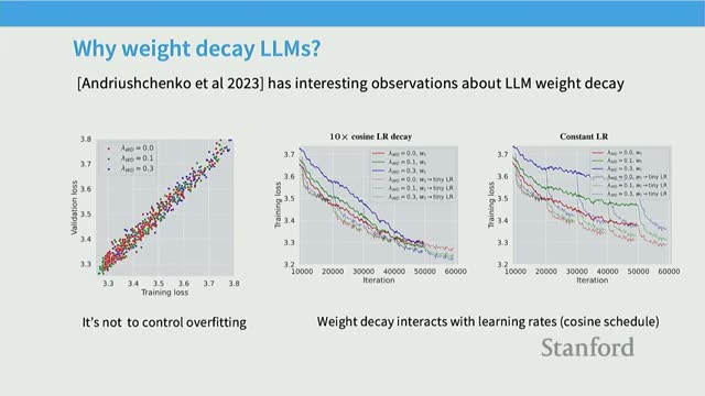
Regularization practice in contemporary pretraining:
-
Dropout is less prevalent in modern pretraining because massive corpora mean models typically do not overfit within a single epoch.
-
Weight decay remains commonly used, not primarily as overfitting control but because it interacts with learning-rate schedules and optimization dynamics to yield better final training loss behavior.
Empirical notes on weight decay:
- It can slow initial progress at high learning rates but enable stronger convergence during late stages as learning rates decay.
- Treat weight decay as an optimization-stability and convergence aid in large-scale pretraining, not exclusively as a regularizer to prevent overfitting.
Consensus hyperparameter defaults as practical starting points
Low-level hyperparameter defaults that emerged from repeated deployments:
- Hidden sizes and head-dimension splits that match systems and parallelism strategies.
- Dff multipliers: ~4× for non-gated, ~8/3× for GLUs.
- Aspect ratios near empirically observed optima.
- Weight decay for stable optimization.
Benefits of using community-validated defaults:
- Provides a robust baseline that reduces tuning cost and instability risk.
- Reflects both representational and systems considerations (memory movement, kernel fusion, parallelism).
When deviating, isolate single changes and re-evaluate optimizer schedules to avoid confounding effects.
Training stability issues concentrate around softmax operations
Softmax operations (final softmax and attention softmax) are common loci for numerical instability due to exponentiation and division.
- These operations can produce large gradients or NaNs during large-scale training, with empirical traces often showing catastrophic spikes in gradient norms associated with softmax computations.
- Interventions that constrain the magnitude of logits or normalize softmax inputs substantially decrease gradient volatility and improve the reliability of long, large-scale training runs.
Addressing softmax-related instability is therefore a central engineering concern when scaling models and datasets.
Z-loss as an auxiliary regularizer for the output softmax
Z-loss augments cross-entropy with a penalty proportional to log(Z(x)), where Z is the softmax normalizer.
- Purpose: encourage the partition function to remain close to one and avoid numerically large logits.
- Effect: reducing the magnitude of log(Z) makes exponentiation/division in the softmax better behaved numerically, lowering overflow and extreme conditioning risk.
- Implementation: an auxiliary term with a small coefficient; used in several large-scale models to stabilize the final softmax and improve training robustness.
When effective, Z-loss acts like encouraging essentially unnormalized scores at the tail end of training to simplify numerical operations.
QK normalization (layer-norm on queries and keys) to tame attention softmax inputs
Applying normalization to queries and keys (Q/K normalization) before computing dot-products bounds the magnitude of logits entering the attention softmax.
- This prevents extreme values from destabilizing exponentiation and controls per-token and per-head variance.
- Benefits: enables more aggressive learning rates and more consistent gradient norms without altering attention semantics beyond stable scaling.
- Origin and adoption: technique used in large vision and multimodal training and adopted by multiple recent language models to reduce attention-induced training spikes.
Because the normalization parameters are learned and kept at inference time, this change improves numerical behavior across training and deployment.
Soft-capping logits as an alternative clipping strategy
Soft-capping applies a smooth, saturating transform (e.g., scaled tanh) to logits before softmax to prevent extremely large values while preserving differentiability.
- The transform maps logits above a chosen soft cap into a bounded range so the softmax denominator stays well-conditioned, reducing NaN and overflow risk.
- Empirical note: effects on final perplexity are mixed—soft-capping can improve stability but may harm optimal loss if applied naively.
- Comparison: QK normalization often allows more aggressive learning rates with better final outcomes.
Recommendation: choose soft-cap thresholds and scaling carefully and validate empirically, since aggressive clipping can impede expressivity.
Inference arithmetic intensity and the motivation for multi-query/group-query attention
Inference generation and KV cache characteristics:
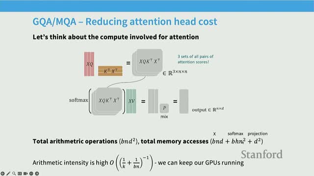
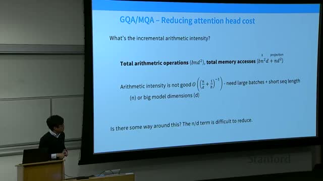
- Autoregressive generation uses sequential computation with a persistent KV cache, producing unfavorable memory-to-compute ratios compared with batch training because each new token requires accessing and updating past keys/values.
-
Arithmetic intensity (compute per memory access) drops dramatically at inference, increasing sensitivity to memory movement and motivating attention designs that reduce per-step memory traffic.
Memory-reducing attention variants:
-
Multi-query attention (MQA): share keys and values across heads while keeping distinct queries.
-
Group-query attention (GQA): share K/V at a coarser granularity.
These variants trade a small change in attention expressivity for substantial reductions in KV cache size, memory movement, and improved latency at long context lengths.
KV cache mechanics and quantitative impact on inference memory and compute
During autoregressive generation the model incrementally appends keys and values to a persistent KV cache and computes one new attention row per token, shifting dominant costs:
- Training is dominated by matrix-matrix multiplies; cached inference is dominated by many vector-matrix and memory-intensive operations.
- The arithmetic intensity for cached inference contains an n/d-like term that can be large for long sequences and moderate model widths, making throughput memory-bound rather than compute-bound.
-
MQA/GQA reduce KV cache size, lowering memory accesses and improving arithmetic intensity by amortizing K/V storage across queries.
Result: very long context lengths become viable while keeping per-token latency and memory footprint manageable. Implementers should evaluate expressivity trade-offs against inference system gains.
Sparse, sliding-window, and hybrid attention patterns for long context
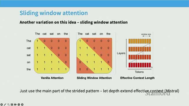
Structured sparse attention and sliding-window patterns reduce quadratic memory costs by limiting attention to local neighborhoods or predefined sparse connectivities.
Design patterns and trade-offs:
- Use sliding-window attention for locality and periodic global/stride-based slots to propagate long-range information.
- Hybrid designs combine occasional full self-attention layers with multiple sliding-window layers and can omit positional encodings on some layers to enable long-range extrapolation and efficient computation.
- Modern long-context models commonly mix sparse/local attention with strategic full-attention checkpoints to balance systems efficiency and global context propagation.
Caveat: designing these patterns requires careful consideration of task locality, layer depth, and the desired extrapolation properties.
Enjoy Reading This Article?
Here are some more articles you might like to read next: