CS336 Lecture 7 - Parallelism
- Lecture overview and objectives
- Motivation for multi-machine scaling from compute requirements
- Memory scaling motivates model sharding across devices
- Hardware hierarchy and interconnect tiers influence parallelization choices
- Collective communication primitives and their equivalences
- Differences between GPU and TPU networking and implications for collectives
- Data center as the new unit of compute and collective-centric performance reasoning
- Three high-level parallelism axes: data, model, and activation
- Naive data parallelism implements synchronous SGD with full-parameter replication
- Data-parallel tradeoffs: compute saturation versus communication and memory replication
- Optimizer-state explosion and its impact on memory
- ZeRO stage 1 (optimizer state sharding) reduces per-device optimizer memory by sharding state
- ZeRO stage 2 shards gradients incrementally during backward pass to limit peak memory
- ZeRO stage 3 / FSDP fully shards parameters, gradients, and optimizer state with on-demand parameter communication
- Practical performance of ZeRO stages and memory efficiency examples
- Batch size is a limited resource that constrains data parallel scalability
- Model parallelism partitions model state across devices to reduce memory and activation cost
- Pipeline parallelism partitions layers across devices and exposes pipeline bubbles
- Zero-bubble (dual) pipelining reduces idle time by rescheduling weight-gradient computations
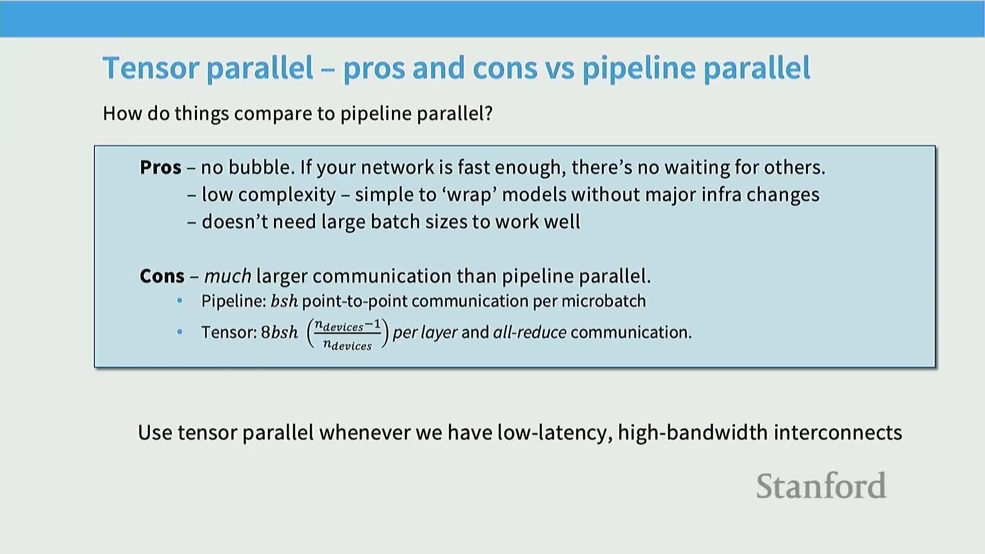
- Tensor parallelism splits large matrix multiplies into submatrices and uses collective sums
- Comparing pipeline and tensor parallelism and common combinations
- Activation memory is dynamically large and can dominate peak memory usage
- Activation memory per-layer formula and the residual ‘straggler’ terms after tensor parallelism
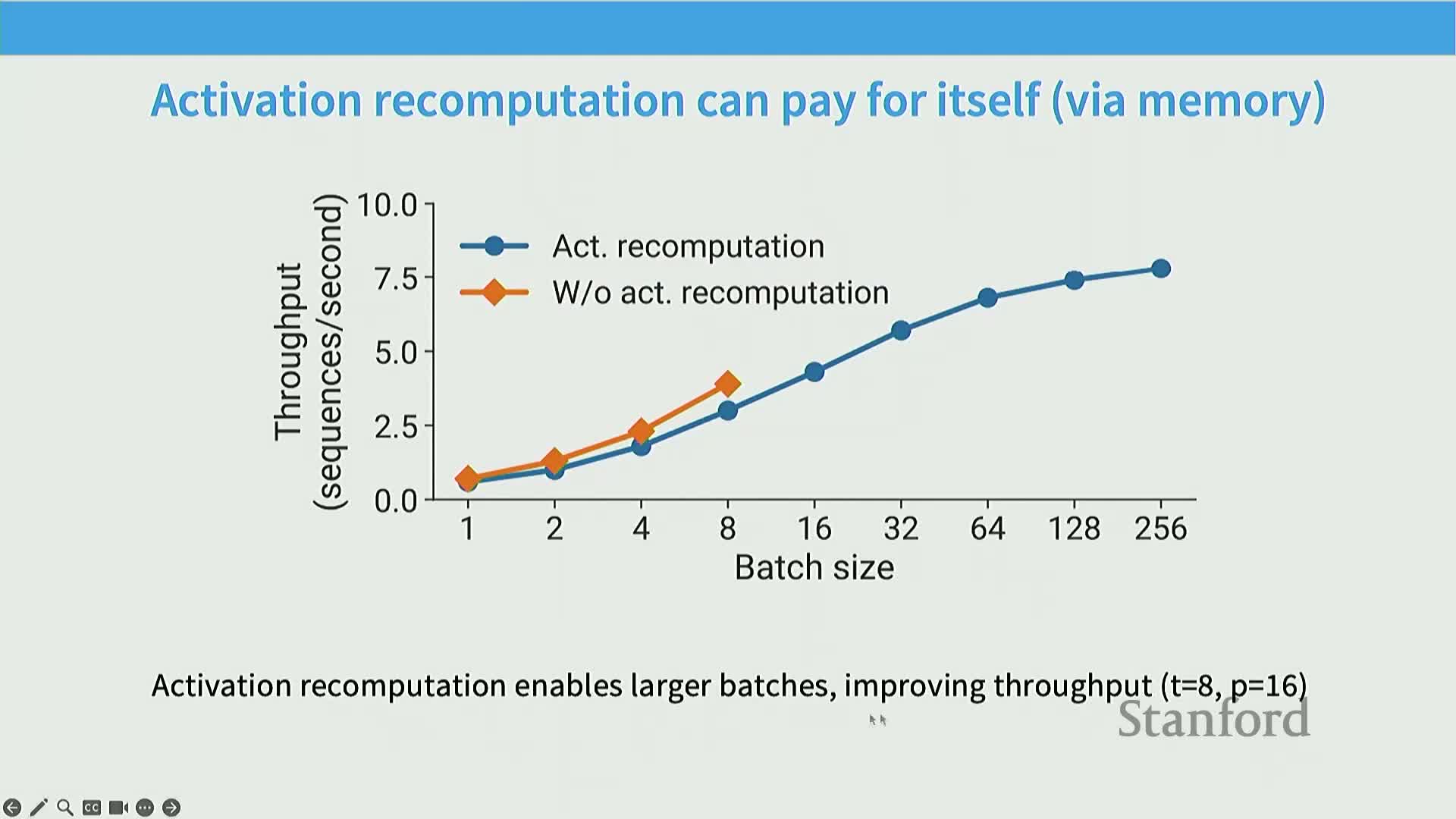
- Sequence-parallel (activation) sharding and recomputation minimize activation memory
- Additional parallelism variants: ring (context) attention and expert (sparse) parallelism
- Tradeoffs summary across distributed-parallel strategies
- Batch-size-to-device ratio determines which hybrid parallelism is optimal
- Practical rule-of-thumb for multi-dimensional parallelism (3D/4D)
- Case studies: Megatron-LM, DeepSeek, LLaMA 3, and TPU-based examples
- Operational challenges at scale including hardware failures and data integrity
- Final synthesis: combine parallelism axes and follow simple rules of thumb
Lecture overview and objectives
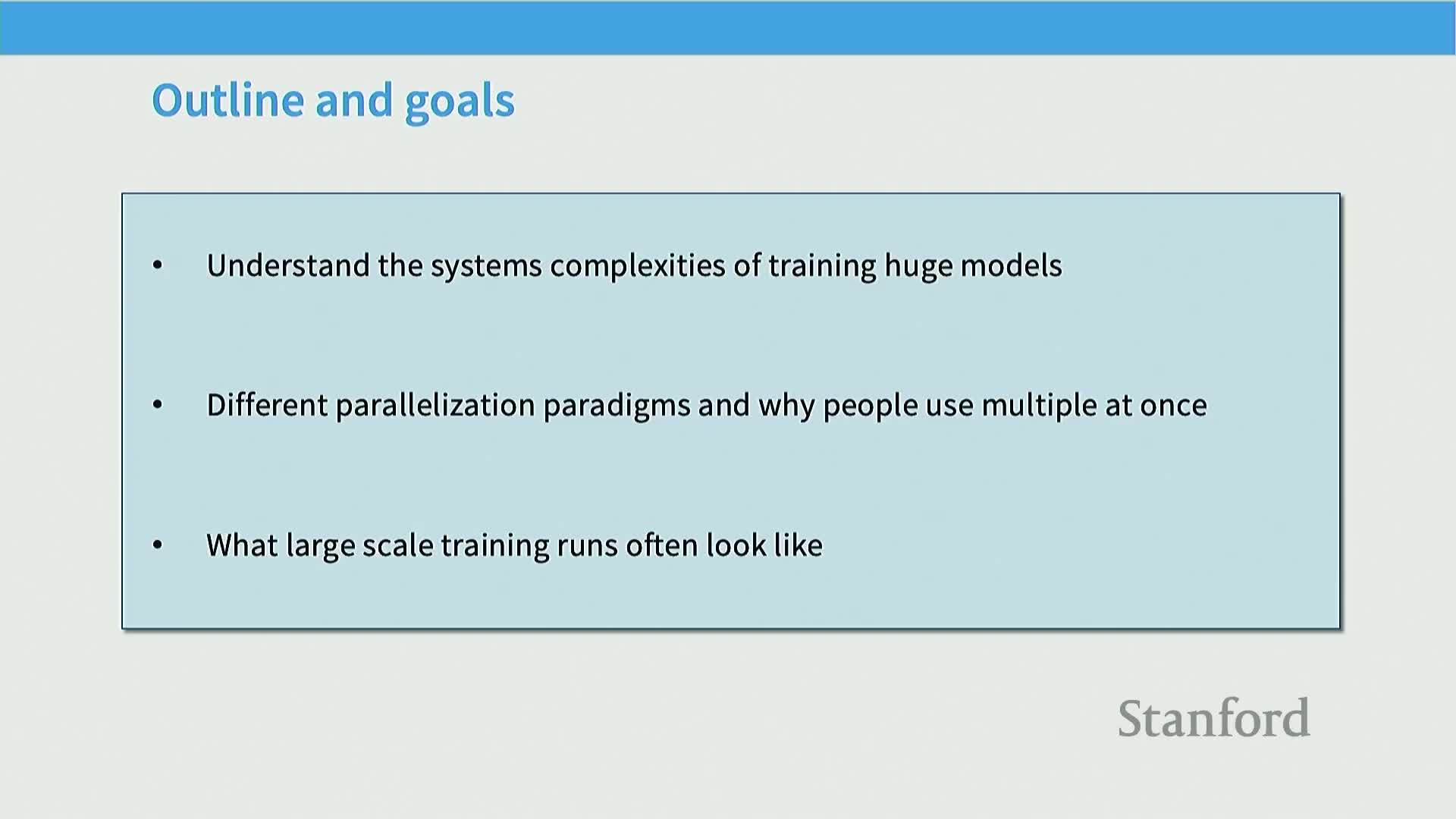
The lecture introduces multi-machine optimization for training very large machine learning models, focusing on parallelism across machines to address compute and memory constraints.
It reframes the problem as moving beyond single-GPU throughput optimization to using multiple servers and accelerators, and stresses that communication patterns and hardware topology critically determine which parallelization techniques are effective.
Planned coverage:
- Networking basics (interconnect hierarchies and their costs)
- Parallelization paradigms (data, model, activation/sequence axes)
-
Case studies and practical heuristics for combining techniques to fit models that do not fit on a single GPU while maximizing throughput and respecting memory limits
Objective: combine different parallelization strategies to train models that exceed single-GPU capacity while maximizing throughput and honoring memory limits.
Motivation for multi-machine scaling from compute requirements
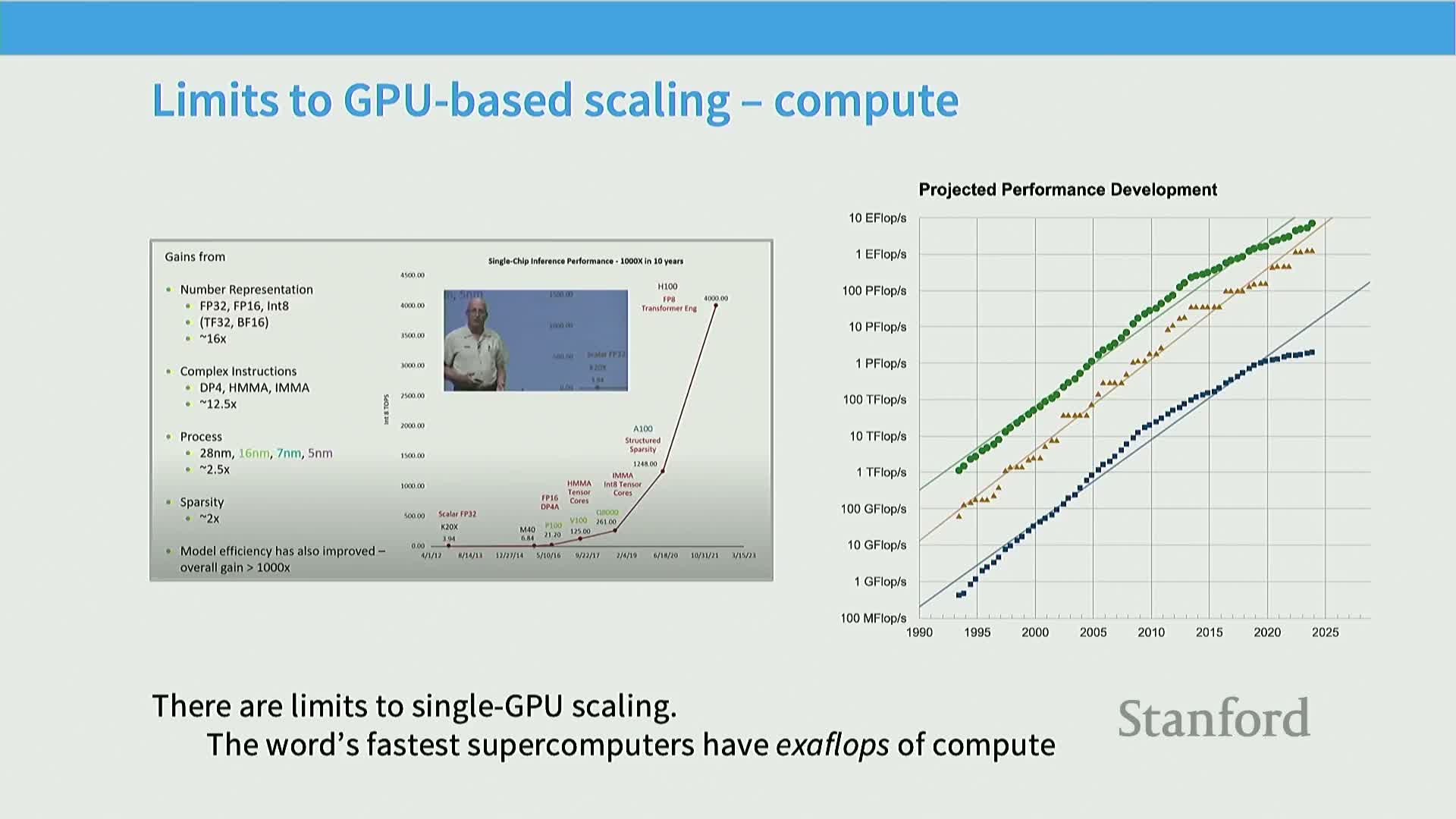
Large-scale language models require aggregate compute that outpaces single-GPU FLOPS growth, so distributed multi-machine systems are necessary to reach exascale-class training throughput.
Key points:
- High-end supercomputers demonstrate that state-of-the-art training requires distributing compute across many nodes rather than waiting for single-device advances.
- Investing in multi-node parallelism unlocks orders-of-magnitude more FLOPS than any single accelerator.
This compute motivation justifies the forthcoming discussion of distributed algorithms and system-level tradeoffs that enable large-model training.
Memory scaling motivates model sharding across devices
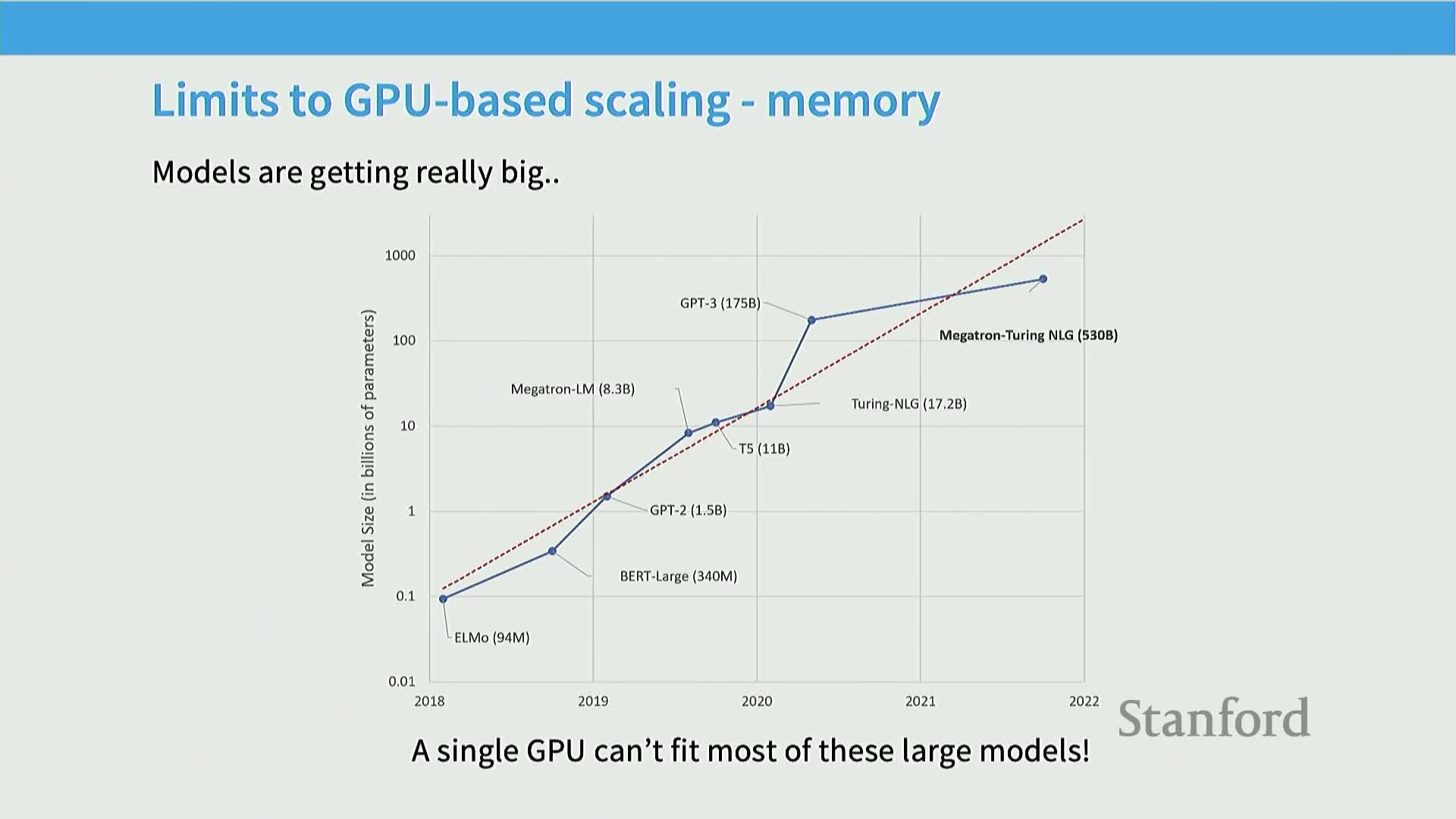
Model parameter counts are growing faster than individual accelerator memory, so billions-parameter models routinely exceed a single GPU’s capacity and must be distributed across devices.
Implications and strategies:
- Accelerator memory increases slowly relative to model size → a hard constraint requiring sharding techniques for parameters, optimizer state, and activations.
- Addressing memory scaling is as important as compute scaling: models need both capacity for parameters and working memory for optimizer state and activations.
- Common strategies motivated by memory pressure: optimizer-state sharding, parameter sharding, activation management, and other memory-saving techniques.
Hardware hierarchy and interconnect tiers influence parallelization choices
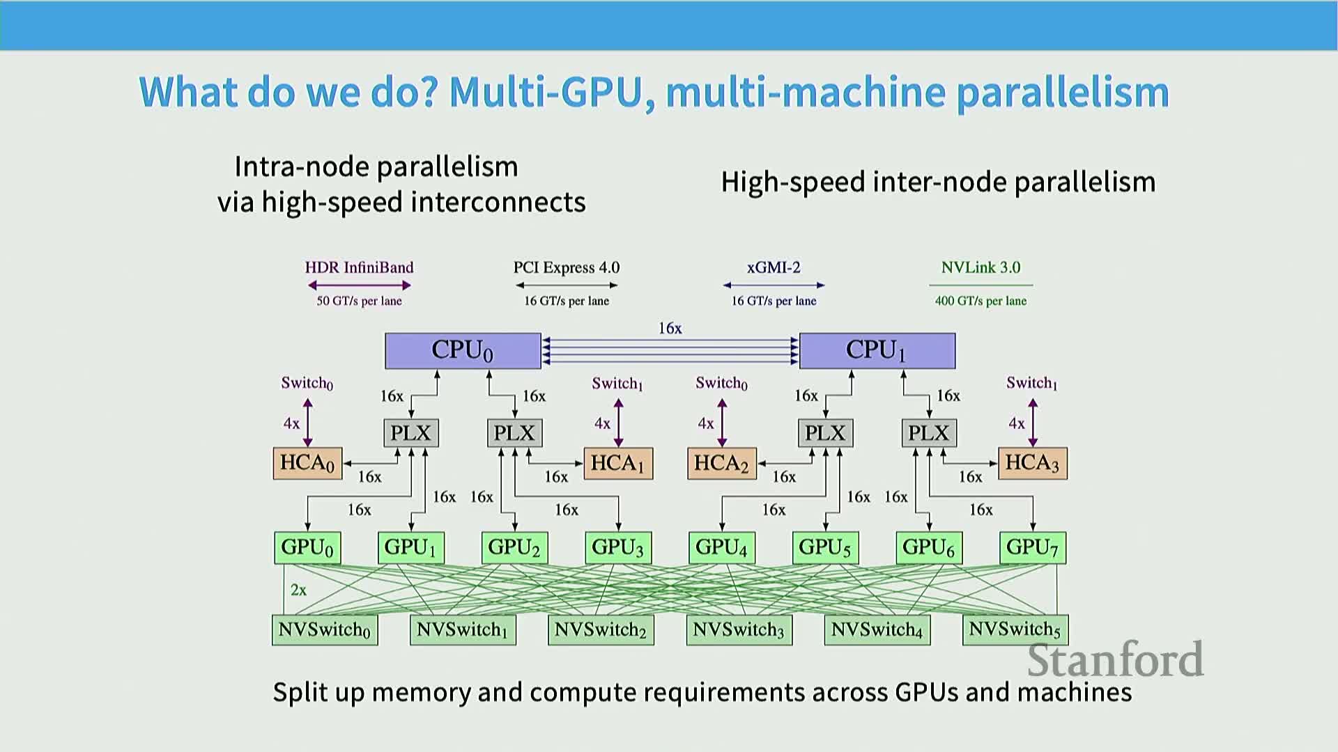
Hardware topology creates a strong communication-performance gradient that drives placement decisions.
Highlights:
- Node-local interconnects (e.g., NVLink, NVSwitch) provide very high bandwidth and low latency between GPUs within a machine.
- Inter-node links (e.g., HDR InfiniBand) are substantially slower; cross-rack or large-scale switches can be slower still.
- Result: intra-node collectives are much cheaper than inter-node collectives, and performance can shift again beyond ~256 GPUs due to differing switch fabrics.
Design rule: place bandwidth-hungry synchronizations inside the fast connectivity domain and minimize or restructure communication across slower links. This explains rules of thumb like applying tensor-parallel techniques within a node and using data or pipeline parallelism across nodes.
Collective communication primitives and their equivalences
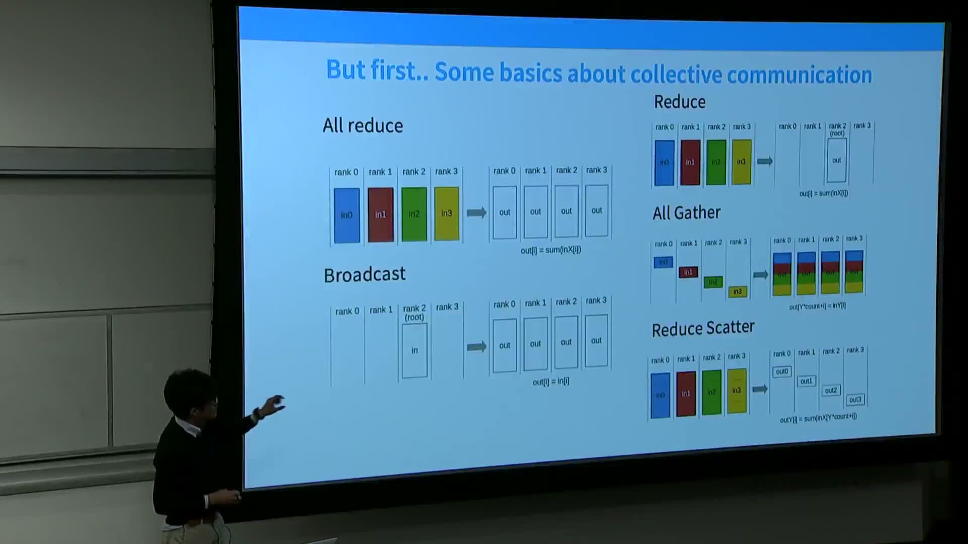
Distributed training communication cost can be modeled by counting collective primitives, because most parallel algorithms compose these operations.
Common collectives (with short descriptions):
- All-reduce: compute a global reduction (e.g., sum) and distribute the result to all ranks.
- Broadcast: copy a single rank’s tensor to all ranks.
- Reduce: gather and reduce inputs to a single rank.
- All-gather: concatenate shards from all ranks into full tensors on every rank.
-
Reduce-scatter: perform a reduction and distribute different output shards to different ranks.
Practical note: in bandwidth-limited regimes, all-reduce ≈ reduce-scatter followed by all-gather, so counting these primitives gives a good first-order model for communication overhead in parallel training.
Differences between GPU and TPU networking and implications for collectives
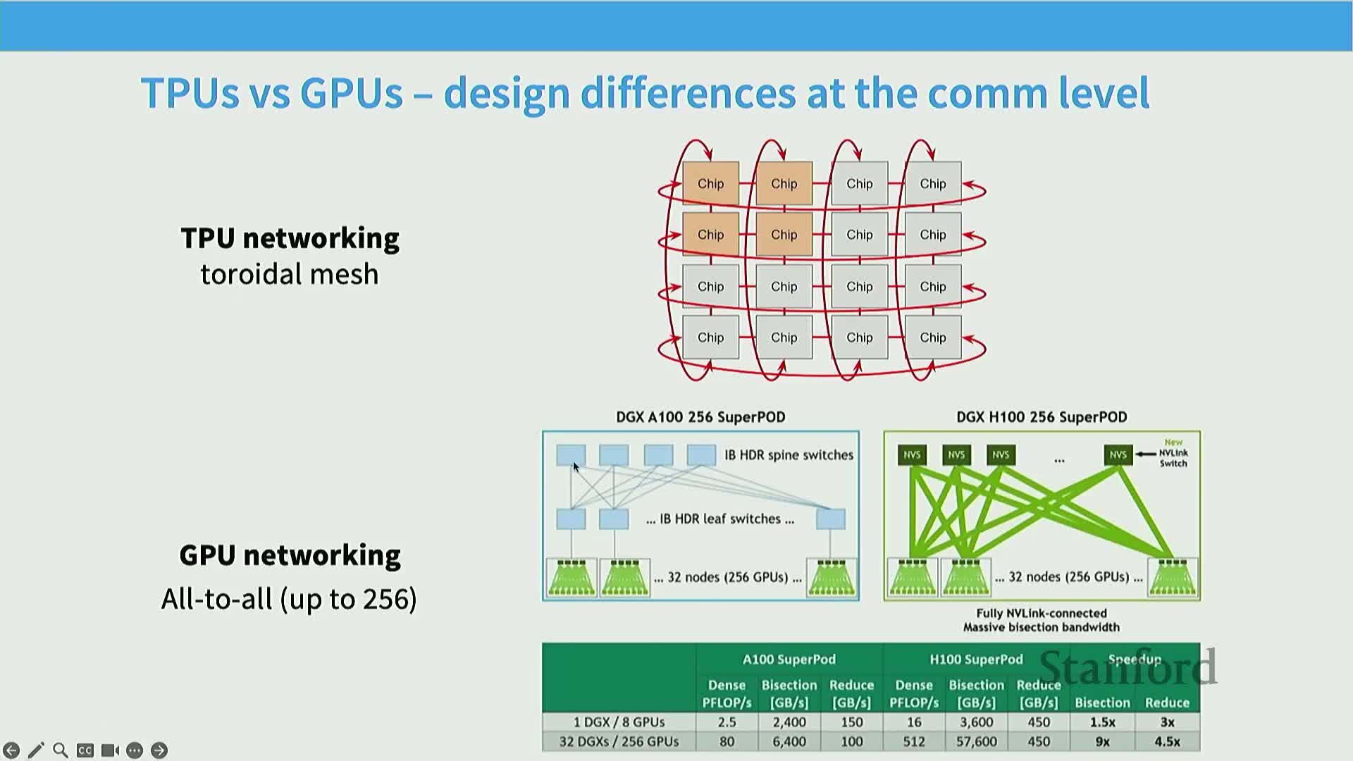
Different accelerator/network architectures favor different communication patterns and therefore different parallel algorithms.
Comparison:
- GPU-based clusters: node-centric high-speed links plus slower inter-node fabrics → arbitrary communication patterns up to a scale.
-
TPU-style toroidal mesh: neighbor-to-neighbor high-bandwidth links favor locality and neighbor-based collective algorithms.
Implications:
- Collective-heavy workloads can benefit from torus-like topologies at scale.
-
Heterogeneous or irregular communication patterns often favor GPU cluster fabrics with broader connectivity.
Choice of accelerator and network topology influences optimal system design and parallelism choices.
Data center as the new unit of compute and collective-centric performance reasoning
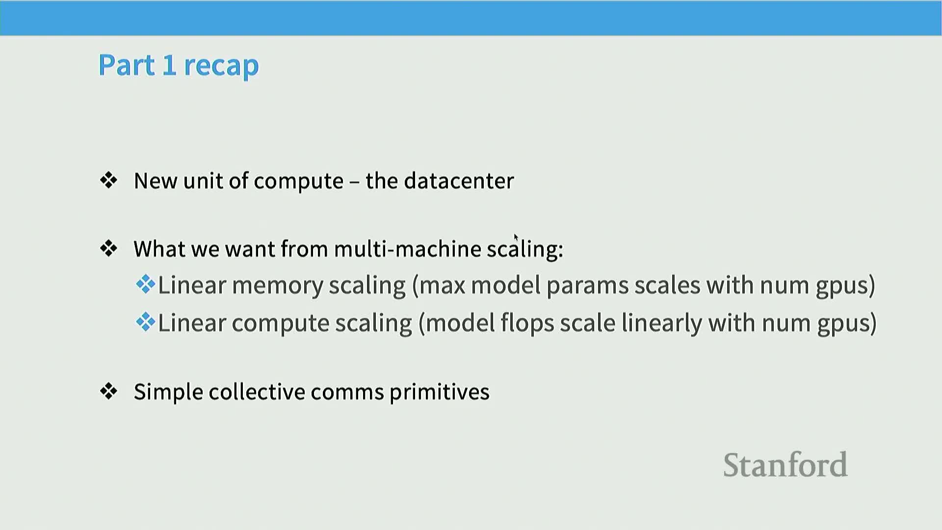
At datacenter scale, the unit of computation becomes the entire cluster, and scalable algorithms aim for linear scaling of both usable model size (memory) and aggregate compute with the number of devices.
Design goals and modeling approach:
- Achieve linear memory scaling (train larger models) and linear compute scaling (increase effective throughput).
- Use collective-primitive counting as the primary performance model because many algorithms are built from those building blocks.
Reasoning about the number and type of collectives is sufficient for estimating bandwidth-limited performance at scale.
Three high-level parallelism axes: data, model, and activation
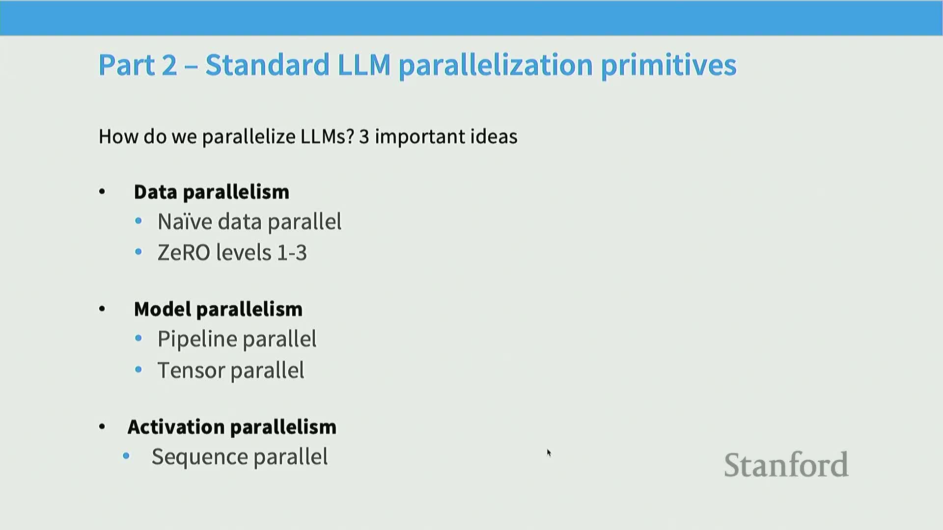
Scaling strategies decompose into three fundamental axes: data parallelism, model parallelism, and activation (sequence) parallelism.
Definitions:
- Data parallelism: replicate parameters and shard minibatches across replicas; synchronize gradients.
- Model parallelism: shard parameters across devices (e.g., pipeline or tensor parallelism); transfer activations between devices.
-
Activation (sequence) parallelism: shard activations across devices or time (sequence positions) to reduce activation memory.
Combining these axes provides the tools to jointly scale compute and memory while balancing communication, computation, and batch-size constraints.
Naive data parallelism implements synchronous SGD with full-parameter replication
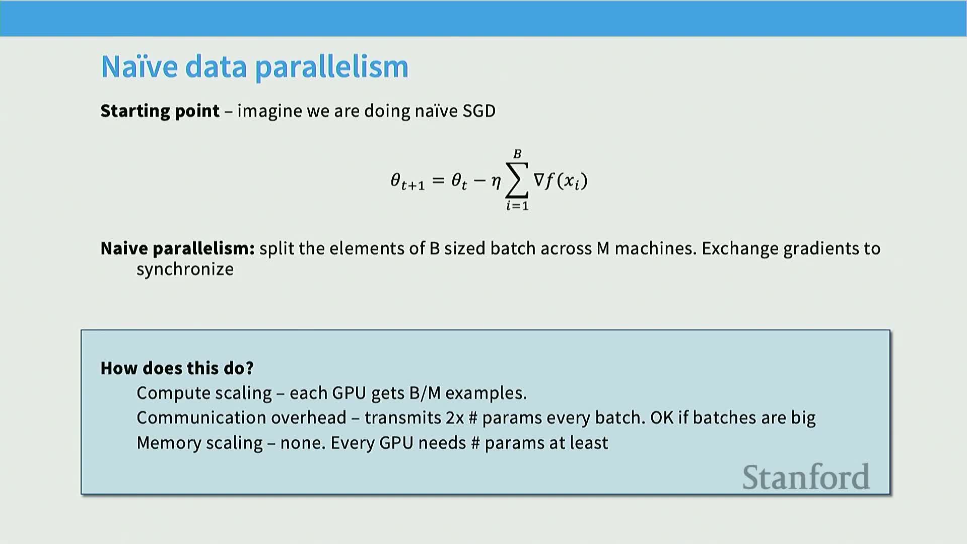
Naive data parallelism workflow (synchronous):
- Split each minibatch into M micro-batches and send one micro-batch to each device.
- Place identical model replicas on each device and compute per-device gradients.
- Synchronize gradients via an all-reduce across replicas.
- Perform the parameter update on each replica.
Properties:
- Near-linear compute scaling when each device receives a sufficiently large micro-batch to saturate compute.
- Poor memory scaling because parameters and optimizer state are replicated on every device.
- Communication overhead ≈ twice the model parameter size per update in bandwidth-limited all-reduce regimes.
- Assumes sufficiently large global batch sizes to amortize synchronization costs.
Data-parallel tradeoffs: compute saturation versus communication and memory replication

Practical limits of naive data parallelism:
- Good compute scaling only when micro-batches per device are large enough to utilize accelerators.
- Communication cost grows with model size and occurs every synchronous step.
- Memory scaling is unfavorable: every device stores full parameters and optimizer state (often multiple copies), which is problematic for optimizers like Adam.
- Conclusion: naive data parallelism is simple and effective up to a point but insufficient when model+optimizer-state exceed single-device capacity or when communication dominates.
Optimizer-state explosion and its impact on memory
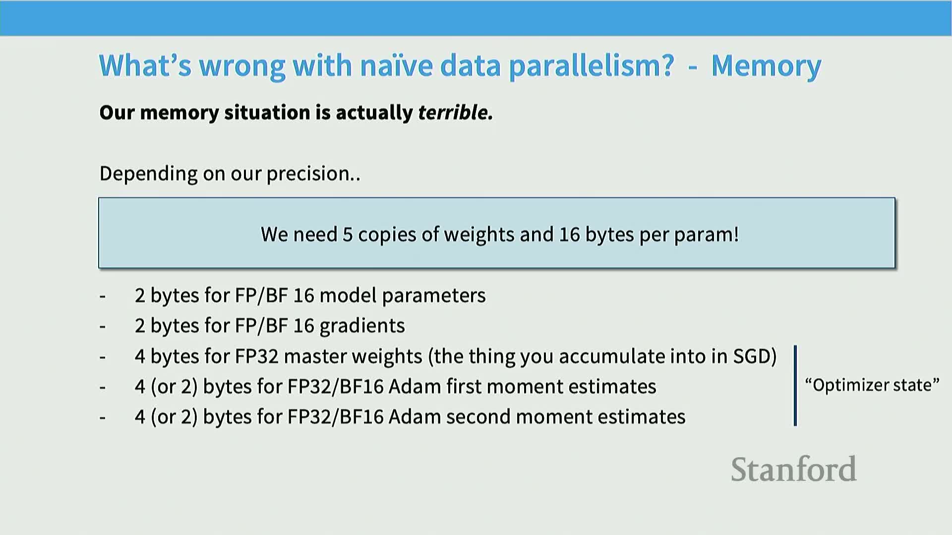
Modern optimizers increase per-parameter memory requirements significantly.
Details:
- Optimizers like Adam require storing first and second moments and often master weights, which can multiply per-parameter memory by factors approaching eight compared to one parameter copy.
- In mixed-precision training, master weights + gradients + moments can produce effective overheads on the order of ~16 bytes per parameter in some implementations.
- Because of this optimizer-state dominance, replicating parameters across devices is frequently infeasible for very large models; addressing optimizer-state memory is a prerequisite to multi-billion-parameter scaling.
ZeRO stage 1 (optimizer state sharding) reduces per-device optimizer memory by sharding state
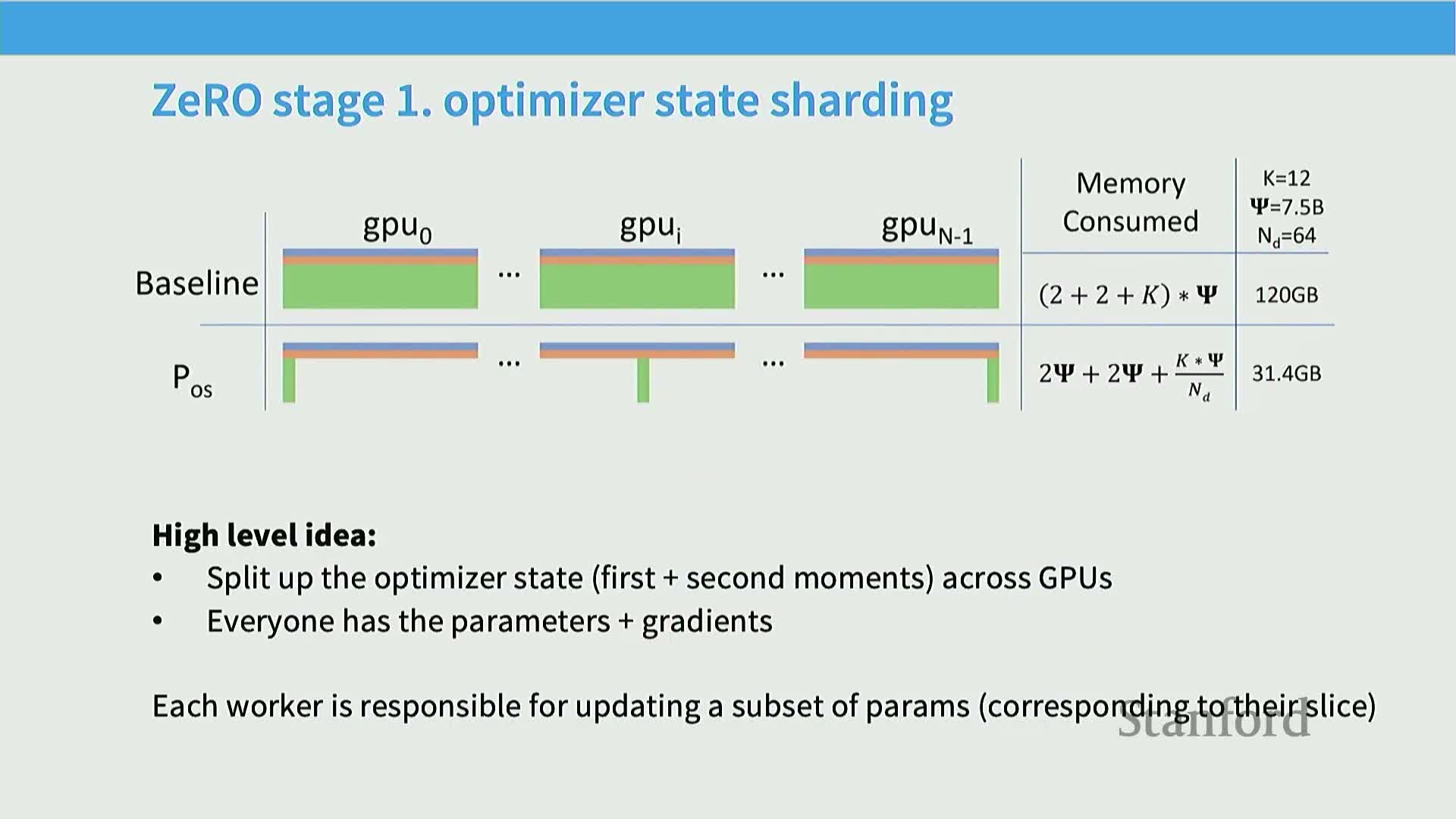
ZeRO Stage 1 shards optimizer-state tensors (e.g., Adam moments) across devices while still replicating parameters and gradients, reducing per-device memory without changing gradient semantics.
Core mechanism (high-level steps):
- Gradients are computed on all devices.
- Use reduce-scatter to aggregate the summed gradients for each parameter shard onto its owning device.
- The owning device updates its local shard with its local optimizer state.
- Use all-gather to distribute updated parameter shards back to replicas.
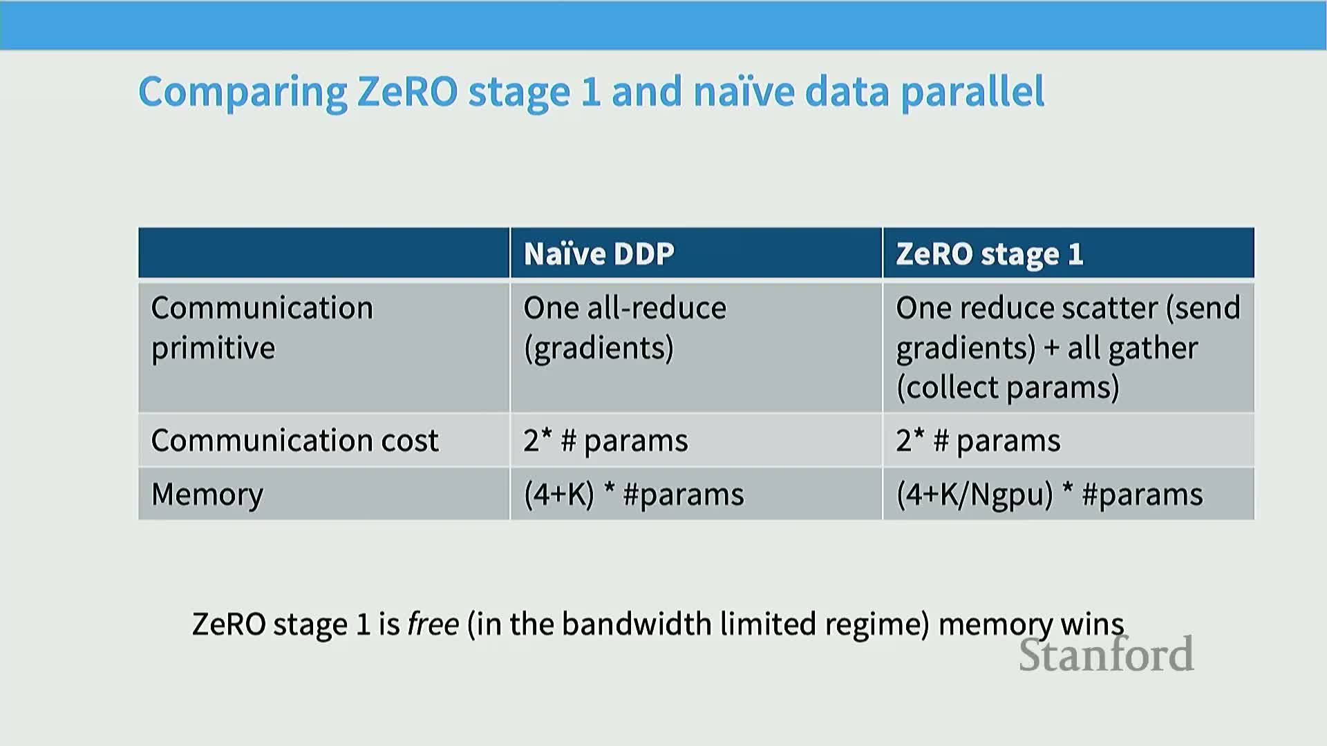
Notes: in bandwidth-limited regimes this sequence (reduce-scatter → local update → all-gather) matches the communication cost of a traditional all-reduce but lowers memory by removing replicated optimizer state.
ZeRO stage 2 shards gradients incrementally during backward pass to limit peak memory
ZeRO Stage 2 extends stage 1 by also sharding gradients so no device materializes the full gradient vector, bounding peak memory usage.
Key behavior:
- During the backward pass, layers are processed sequentially and gradient contributions for a layer are immediately sent (via reductions) to the device that owns the corresponding parameter shard.
- Once a layer’s gradients are communicated and incorporated, local gradient buffers are freed to keep memory low.
- This streaming approach requires more frequent, fine-grained synchronization (layer-by-layer reduces and frees) but keeps the same total communication volume while lowering peak memory compared to stage 1.
ZeRO stage 3 / FSDP fully shards parameters, gradients, and optimizer state with on-demand parameter communication
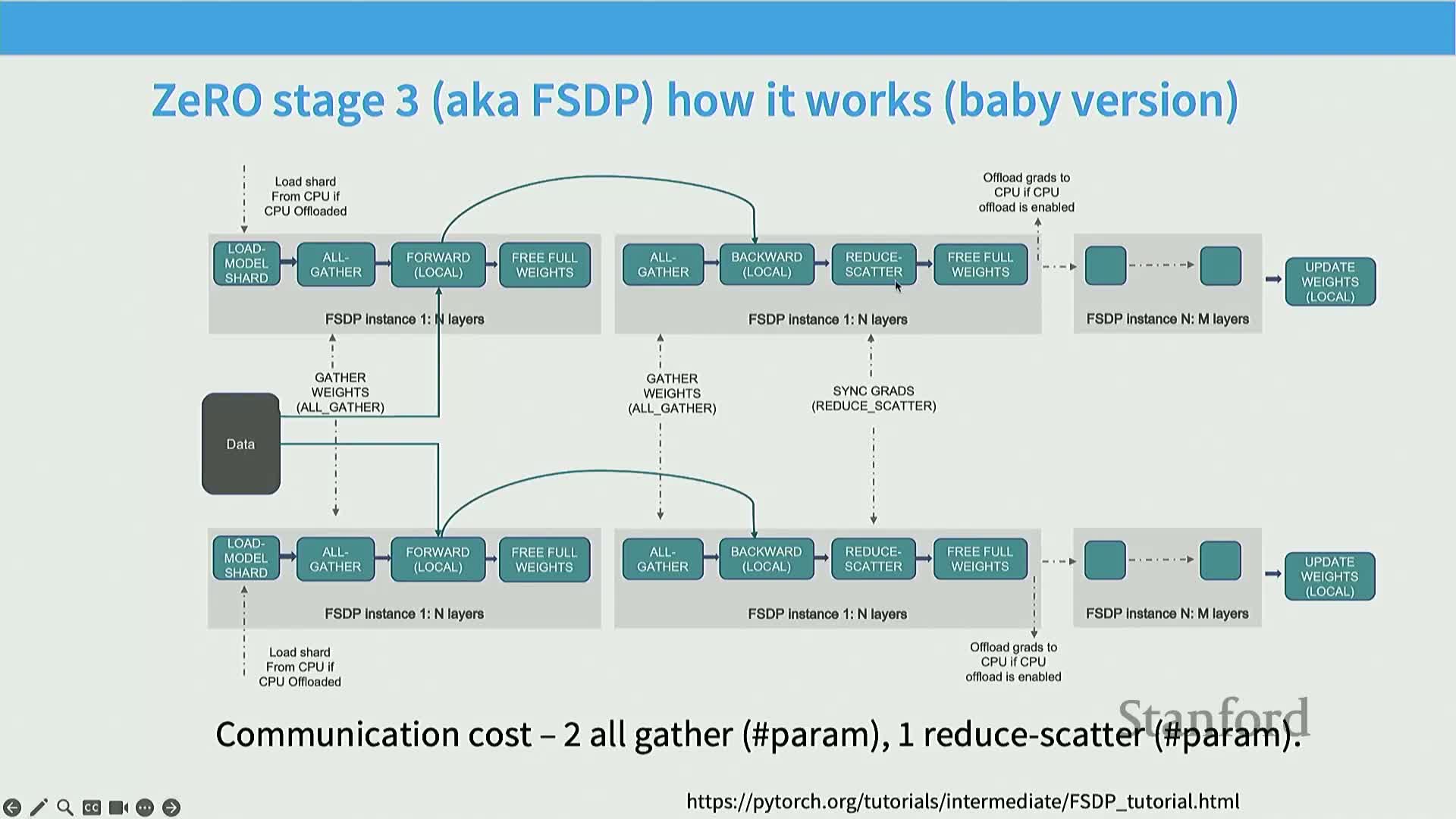
ZeRO Stage 3 (fully-sharded data parallel; e.g., FSDP) shards parameters, gradients, and optimizer state so each device holds only its parameter shard.
Runtime behavior and optimizations:
- During forward/backward, parameters are requested and communicated on demand for local computation.
- The runtime overlaps communication and computation by prefetching parameter shards before they are needed.
- Operations occur at layer granularity using all-gather and reduce-scatter, and shards/gradients are freed immediately after use to minimize memory.
Trade-offs:
- Stage 3 increases the number of collectives (roughly 3× parameter size total bandwidth work vs naive all-reduce’s ~2×), but careful overlap and pipelining keep runtime overhead low in practice while delivering maximal per-device memory savings.
Practical performance of ZeRO stages and memory efficiency examples
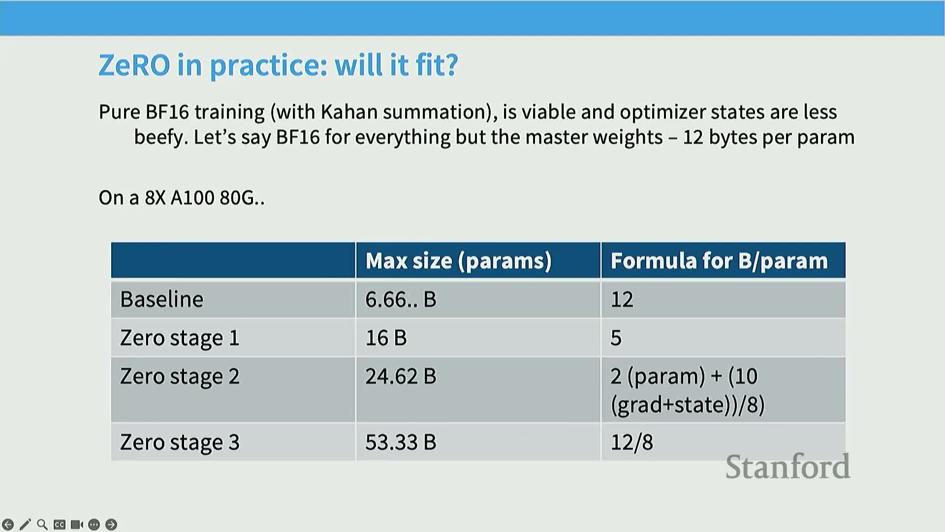
Summary of ZeRO trade-offs:
- Stage 1: memory wins with no extra bandwidth cost compared to standard all-reduce.
- Stage 2: further reduces peak memory via layer-granularity synchronization at the cost of more frequent collects.
-
Stage 3 (FSDP): largest per-device memory reduction but higher total collective count; practical overlap/pipelining often keeps runtime overhead modest.
Practical consequence: full-sharding can enable orders-of-magnitude larger model fits on a fixed node count (e.g., enabling tens of billions of parameters where naive replication would not fit), making ZeRO variants the standard approach when memory is the bottleneck and the extra implementation/communication complexity is acceptable.
Batch size is a limited resource that constrains data parallel scalability
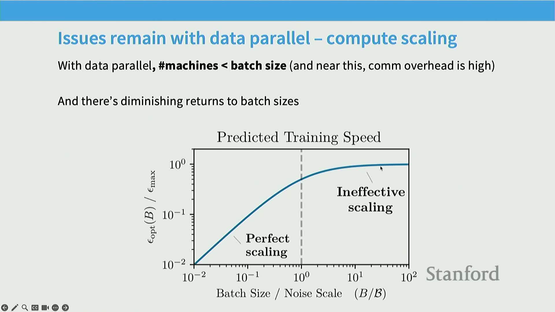
Global batch size constrains how many devices can be used under data parallelism because each device must process at least one micro-batch.
Important points:
- Data parallelism cannot exceed global batch size without gradient accumulation.
- There are diminishing returns: beyond a critical batch size, the marginal benefit of increasing batch size (variance reduction per optimization step) drops sharply.
- Treat batch size as a constrained resource to allocate across parallelism axes.
-
Gradient accumulation trades additional temporal computation for an effectively larger batch size when memory prevents larger per-step batches.
Model parallelism partitions model state across devices to reduce memory and activation cost
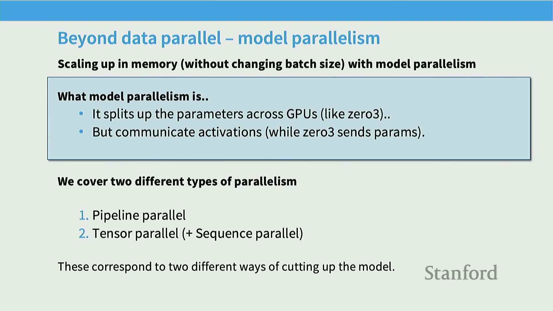
Model parallelism places different parameters on different devices (rather than replicating them), transferring activations between devices instead of parameters.
Main categories:
- Pipeline parallelism: cut the network along depth, assign contiguous layer groups to devices, pass activations forward/backward.
-
Tensor parallelism: split large matrix multiplies across devices and perform partial sums via collectives.
Use cases: model or activation sizes exceed single-device capacity; often combined with data parallelism to achieve both memory and throughput scaling.
Pipeline parallelism partitions layers across devices and exposes pipeline bubbles
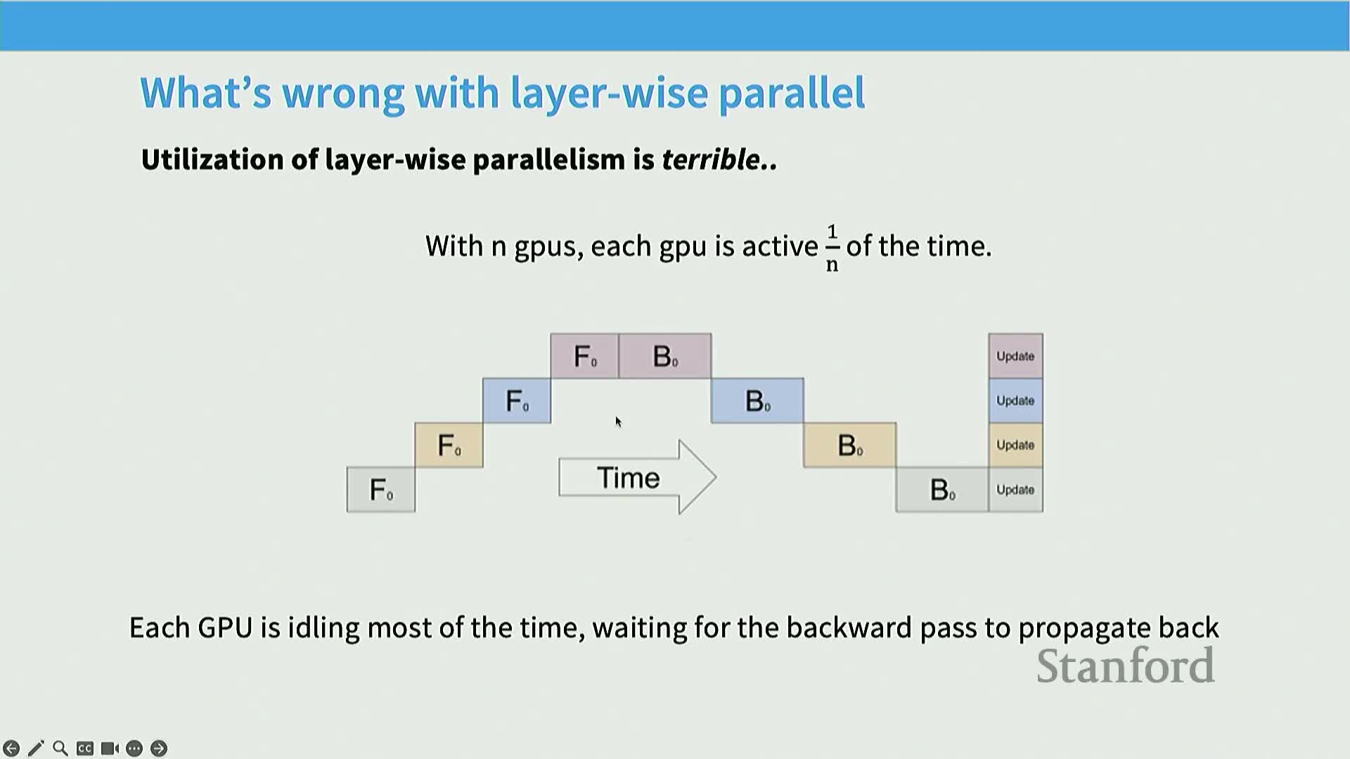
Pipeline parallelism assigns contiguous layer groups to different devices and streams micro-batches through the device pipeline so stages can work concurrently.
Practical considerations:
- Naive scheduling produces pipeline bubbles (idle periods) because stages wait for upstream activations, causing poor utilization when micro-batch counts are small relative to pipeline stages.
- Mitigations: micro-batching (split minibatch into micro-batches) and scheduling strategies like 1F1B to overlap forward/backward passes.
- Pipeline efficiency remains sensitive to micro-batch size and scheduling complexity.
Zero-bubble (dual) pipelining reduces idle time by rescheduling weight-gradient computations
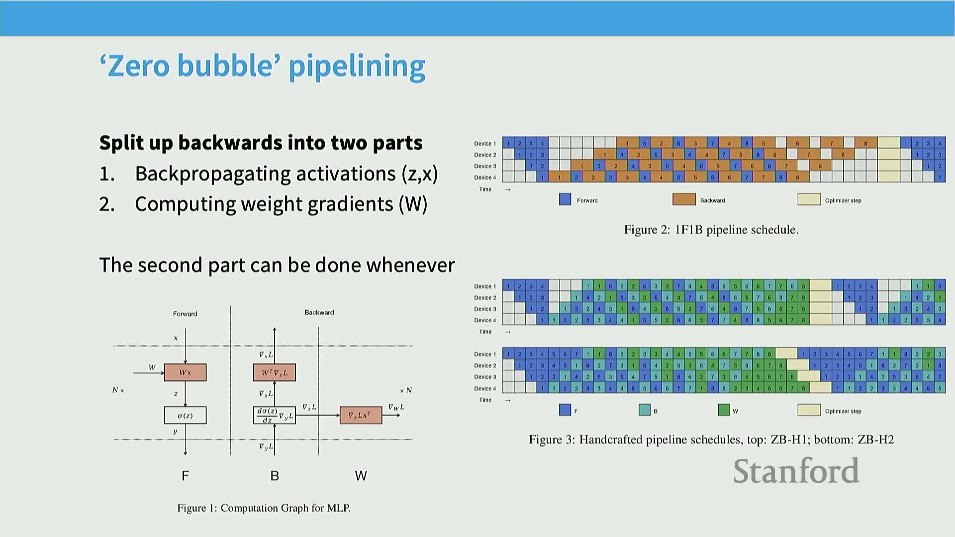
Advanced pipeline optimizations hide idle time by scheduling independent work into pipeline bubbles.
Techniques and trade-offs:
- Split backward work into activation-backpropagation and weight-gradient computation; weight-gradient updates are independent and can fill original pipeline bubbles.
- Methods like dual-pipelining put weight-gradient calculations into otherwise idle slots to improve utilization.
- These techniques increase implementation complexity: manipulating autodiff order, maintaining fine-grained task queues, and ensuring correctness under dynamic scheduling—powerful but operationally costly.
Tensor parallelism splits large matrix multiplies into submatrices and uses collective sums
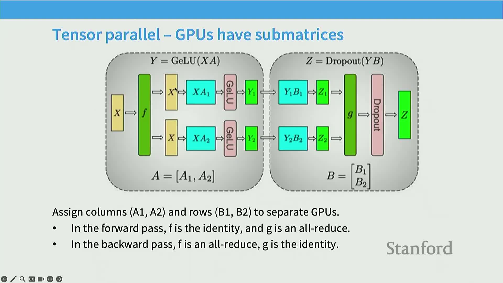
Tensor parallelism partitions the width (or height) of large linear transforms across devices: each device holds submatrices, computes local partial results, and uses collectives (typically all-reduce) to sum partial activations or gradients.
Characteristics:
- Parallelizes dominant linear algebra kernels and avoids pipeline bubbles because each layer runs in parallel across devices.
- Requires very high interconnect bandwidth and low latency.
- Most efficient within a single node (e.g., up to 8 GPUs over NVLink/NVSwitch) and shows rapidly diminishing throughput across slower inter-node links.
Comparing pipeline and tensor parallelism and common combinations
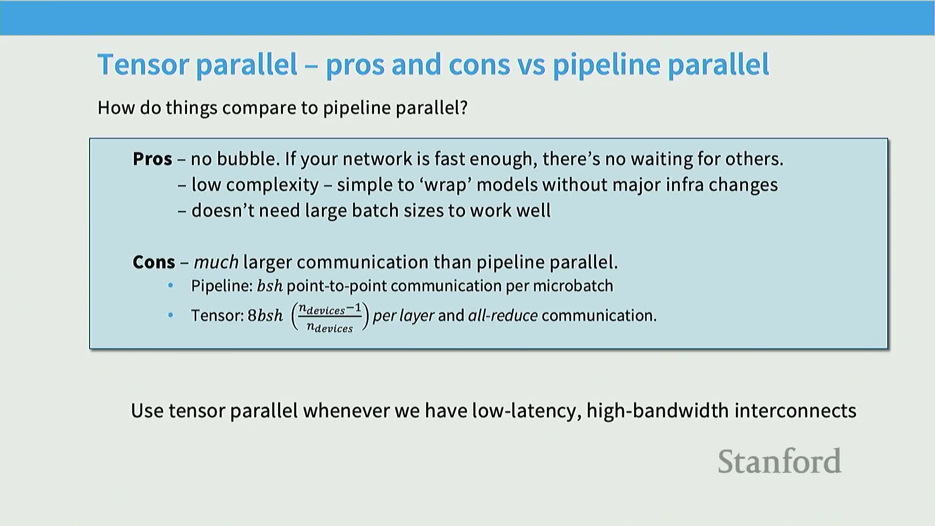
Combining parallelism in real systems:
- Tensor parallelism: applied inside nodes to split matrix computation.
- Pipeline parallelism (and/or model sharding): applied across nodes to stretch model capacity.
-
Data parallelism: layered on top to scale aggregate throughput.
Choice depends on topology, available batch size, and implementation complexity; hybrid strategies are the practical norm.
Activation memory is dynamically large and can dominate peak memory usage
Activation tensors accumulate during the forward pass and are freed during backward, producing dynamic memory profiles where peak memory often occurs mid-backward.
Consequences and mitigations:
- For deep or long-sequence models, activation storage can dominate per-device memory; parameter/optimizer sharding alone does not remove this pressure.
- Techniques to manage activation memory: activation sharding (sequence/position partitioning), recomputation (trade extra compute for reduced storage), and attention-specific optimizations (e.g., flash attention).
Activation memory per-layer formula and the residual ‘straggler’ terms after tensor parallelism
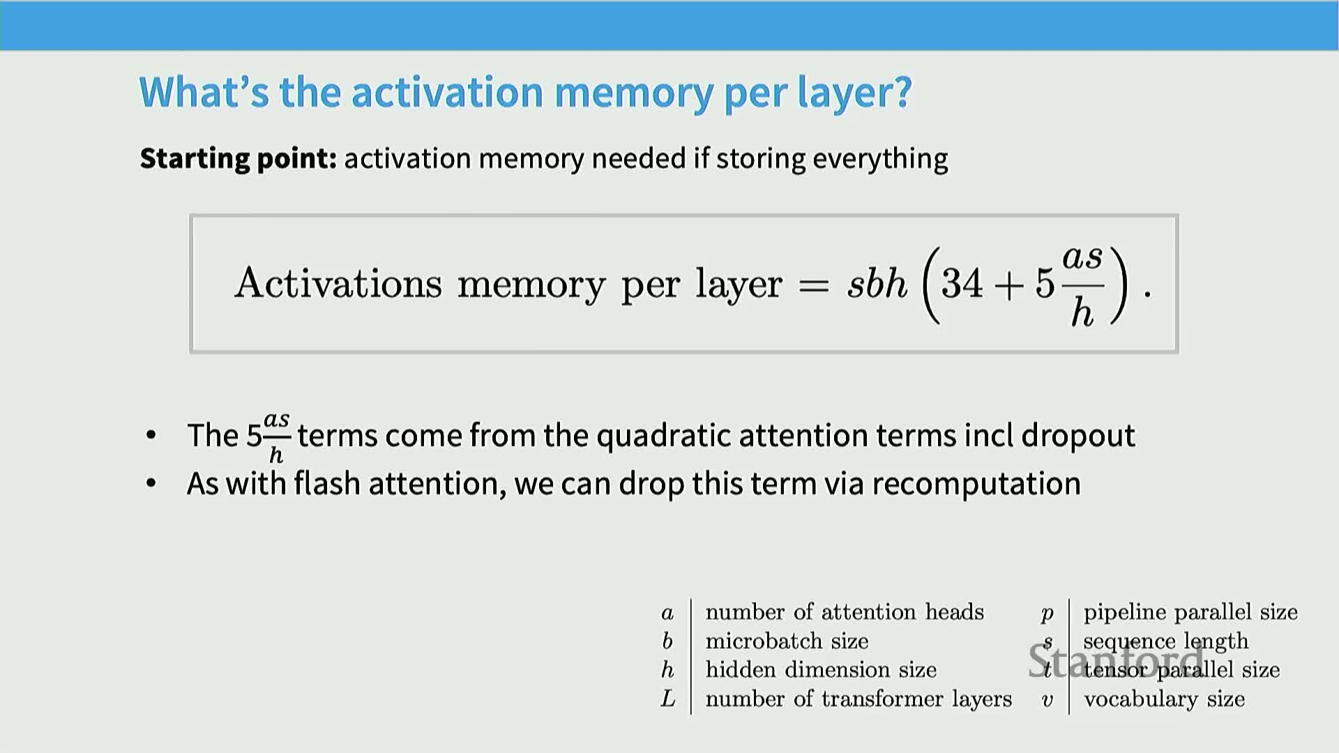
Per-layer activation memory can be approximated by the expression SBH34 + 5A*S/H, where:
- S = sequence length
- B = batch size
- H = hidden size
-
A = attention-cost factor
Interpretation:
- The first term corresponds to MLP and pointwise costs; the second term captures quadratic attention costs.
- Tensor parallelism divides many matrix-related activation terms by the tensor-parallel factor T, but pointwise operations (layer norms, dropouts, small residuals) create a residual SBH*10-like term that does not split cleanly and scales with model size.
- To reduce these straggler terms, apply sequence-parallel techniques (partition activations across sequence positions) and attention recomputation (e.g., flash attention) to lower quadratic memory footprints.
Sequence-parallel (activation) sharding and recomputation minimize activation memory
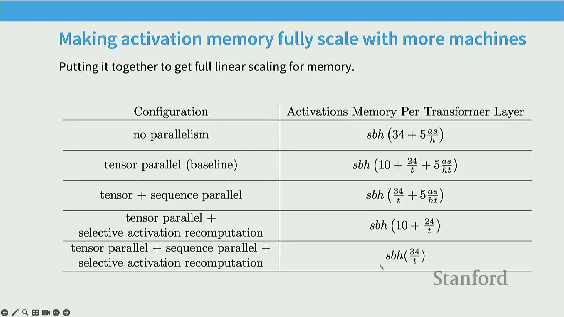
Sequence-parallel and recomputation techniques:
- Sequence parallelism: partition sequence positions across devices so pointwise ops act on disjoint slices; requires all-gather / reduce-scatter at specific points to assemble/distribute tensors for dense ops.
- Activation recomputation: trade extra FLOPS for memory by recomputing intermediate activations on demand instead of storing them.
-
Attention optimizations (flash attention): reduce S^2 memory and compute costs.
Combining tensor parallelism, sequence parallelism, and recomputation approaches a near-minimal activation memory lower bound (roughly SBH*34/T after partitioning), enabling much larger effective models per device.
Additional parallelism variants: ring (context) attention and expert (sparse) parallelism

Variants addressing specific bottlenecks:
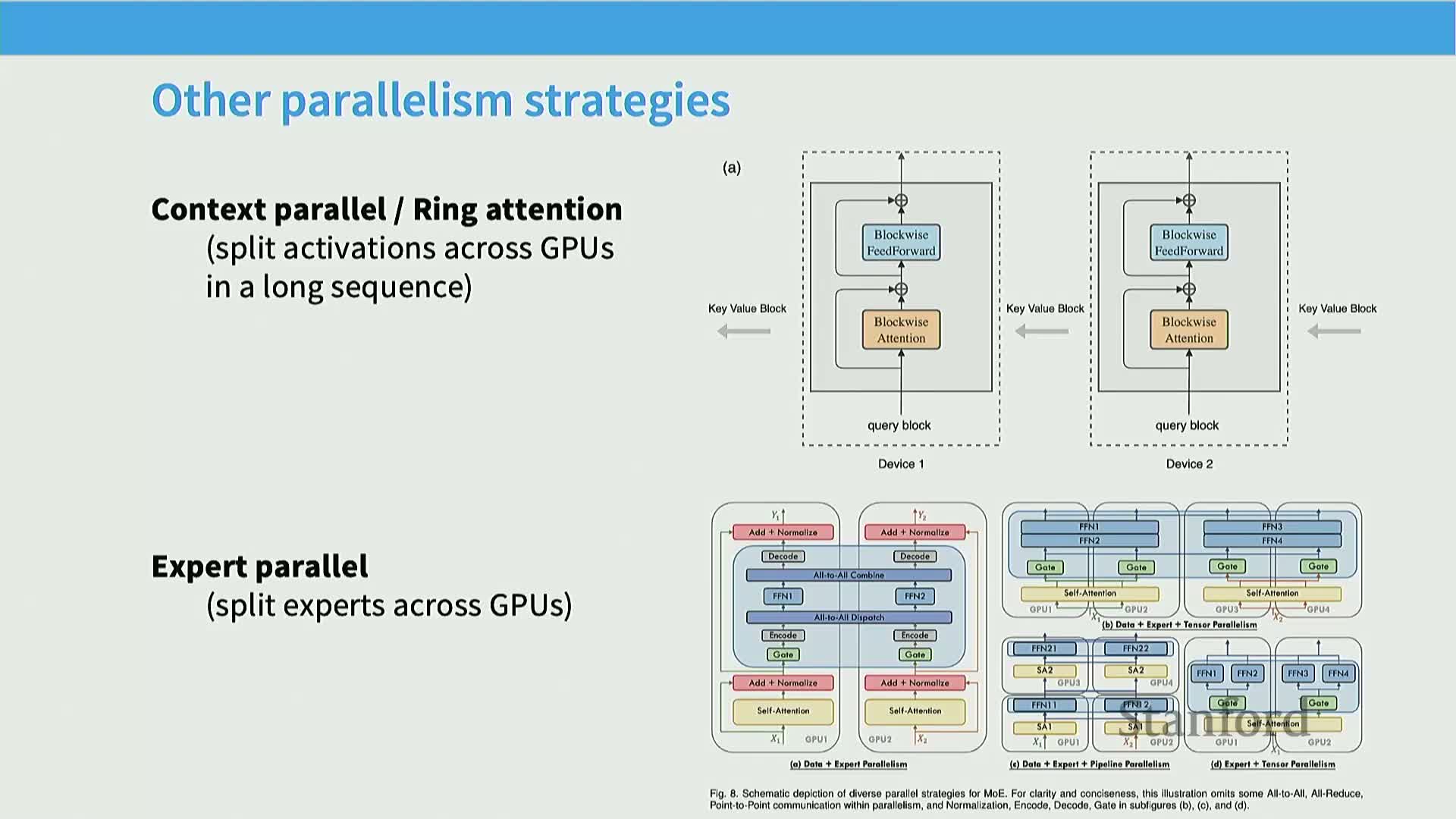
- Ring / context-parallel attention: computes attention by circulating keys/values in a ring so each device handles a subset of queries and receives streamed key-value tiles; reduces per-device memory by using an online tiling pattern (good for long-context attention).
-
Expert parallelism (Mixture of Experts, MoE): partitions MLP capacity into many experts across devices and activates only a sparse subset per input. It resembles tensor parallelism but requires routing mechanisms and load balancing because routing is input-dependent and communication patterns are irregular.
These variants tackle long-context memory (ring attention) and parameter-count scaling with sparsity (MoE), but introduce routing/communication complexity.
Tradeoffs summary across distributed-parallel strategies
Trade-offs across parallelization strategies:
- Data-parallel (DDP): simple and bandwidth-friendly but replicates memory.
- ZeRO / FSDP: reduces memory at modest bandwidth cost and integrates cleanly with existing models.
- Pipeline parallelism: reduces parameter/activation memory per device and can be spread across nodes, but consumes batch-size and is complex to implement.
-
Tensor parallelism: scales matrix computation without consuming batch-size but requires high-bandwidth, low-latency interconnects and frequent collectives.
Selecting a hybrid strategy requires evaluating: network topology, per-device memory limits, global batch-size constraints, and operational cost of implementation and maintenance.
Batch-size-to-device ratio determines which hybrid parallelism is optimal
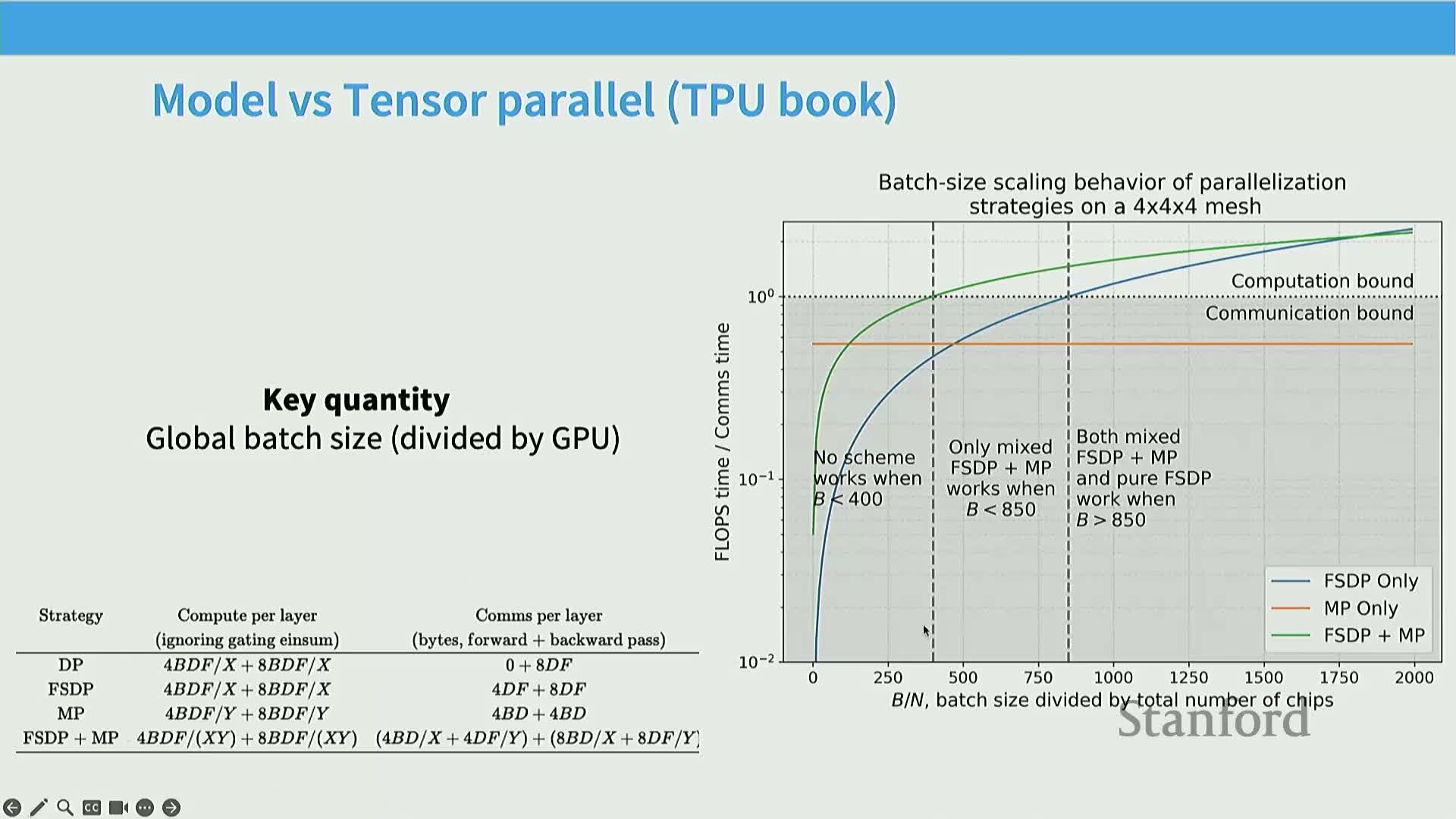
Simple performance model mapping global batch size to parallelism mixes:
- Tiny batch size per device: communication dominates; no technique is efficient.
- Moderate batch sizes: combine ZeRO/FSDP with tensor parallelism to reach compute-bound operation.
-
Large batch sizes: pure data parallelism (or ZeRO with data parallelism) suffices for high utilization.
Practical lever: increasing effective batch size via gradient accumulation trades wall-clock time for improved communication efficiency, so batch-size management is central when tuning parallelism for a hardware fleet.
Practical rule-of-thumb for multi-dimensional parallelism (3D/4D)
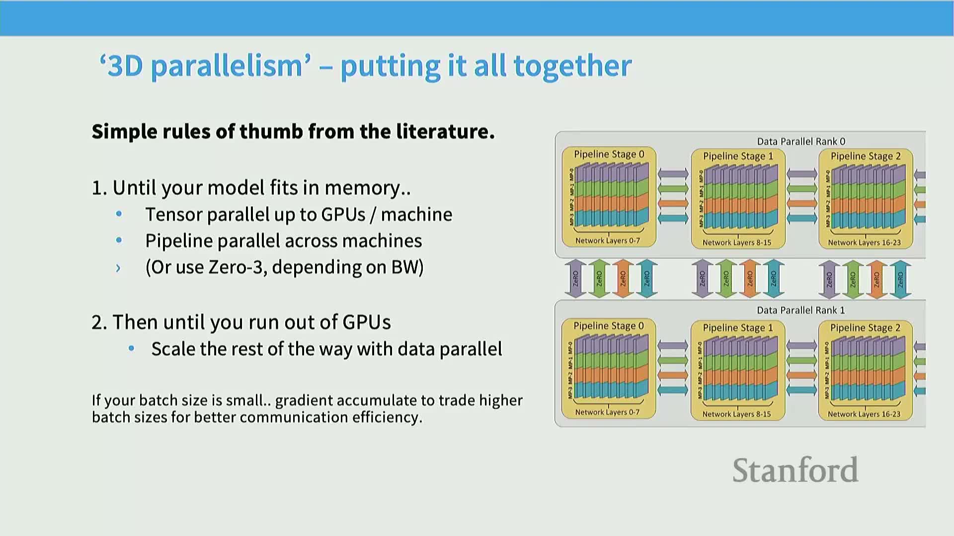
A practical sequence (heuristic) for combining parallelism:
- Fit model and activations in memory using tensor parallelism first (apply up to the number of GPUs per node).
- If needed, use ZeRO Stage 3 (FSDP) or pipeline parallelism across machines to further reduce per-device memory.
- Scale aggregate throughput with data parallelism across many replicas.
- If batch size is insufficient to hide pipeline latency, use gradient accumulation to increase effective batch size and reduce synchronization frequency.
This heuristic often yields near-linear aggregate throughput and provides a reproducible path for choosing which parallelism axes to use at each scale.
Case studies: Megatron-LM, DeepSeek, LLaMA 3, and TPU-based examples
Case study patterns from large-scale training papers and release notes:
- Megatron-LM: tensor parallelism (commonly 1–8-way) combined with pipeline and data parallelism to scale from billions to trillions of parameters.
- DeepSeek variants: mix tensor, sequence, pipeline, and ZeRO Stage 1.
- LLaMA 3: practical combination of tensor parallelism (e.g., 8-way), pipeline stages, FSDP-like sharding, and context-parallel techniques for long-context phases.
-
TPU-based systems (e.g., GMA2): leverage toroidal mesh networking to expand model-parallel extents.
These case studies validate earlier rules of thumb: practical systems almost always combine multiple parallelism axes tailored to hardware and workload.
Operational challenges at scale including hardware failures and data integrity
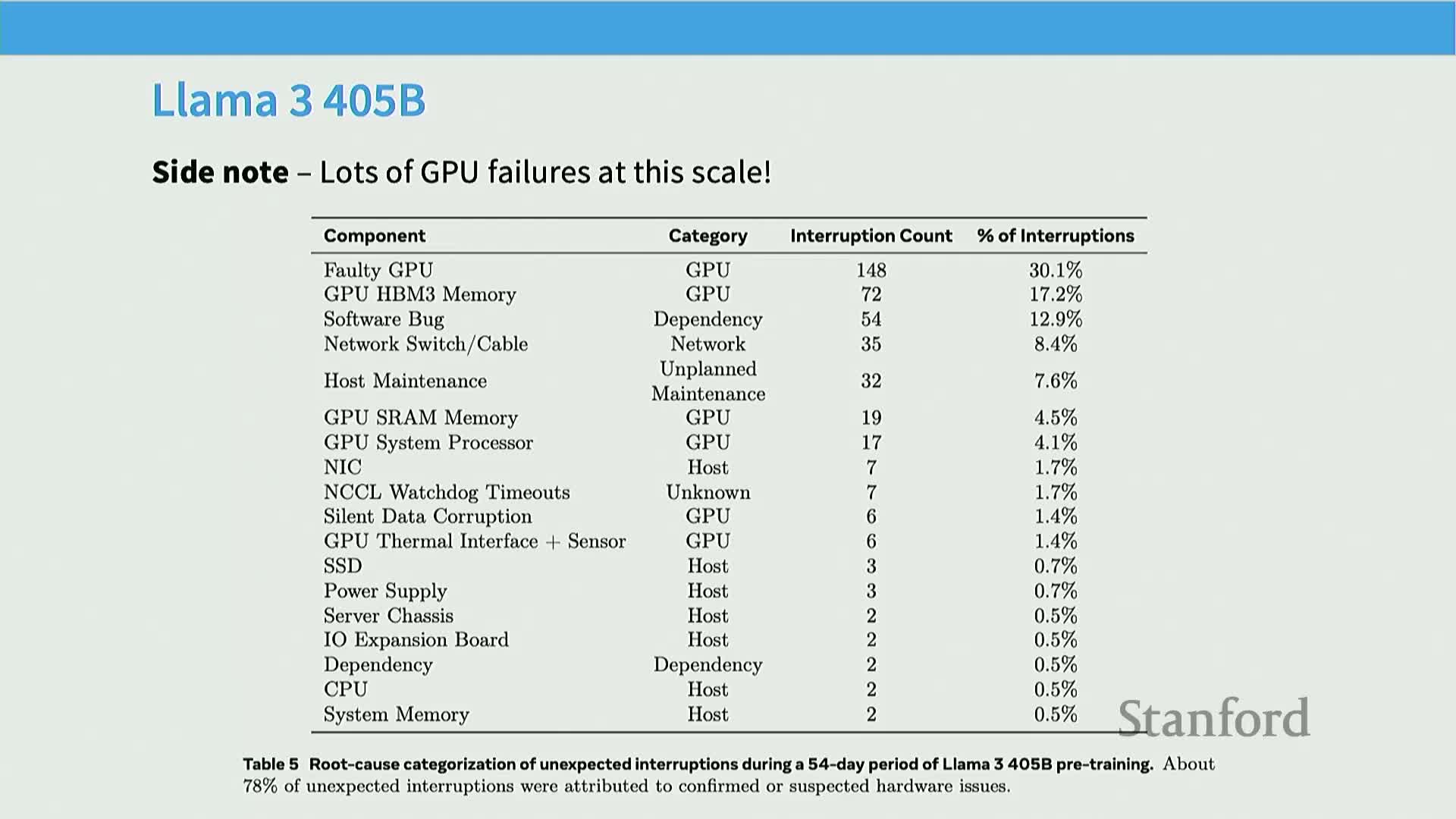
Operational risks and reliability concerns for large-scale distributed runs:
- Common failures: GPU hardware failures, node maintenance interruptions, and silent data corruption. Production runs often see hundreds of interruptions.
- Essential mechanisms: checkpointing, redundancy, validation, and observability to detect silent numerical corruption.
- Operational robustness (fault tolerance, monitoring, and validation) is as important as algorithmic scaling when running multi-week, multi-thousand-GPU training campaigns.
Final synthesis: combine parallelism axes and follow simple rules of thumb
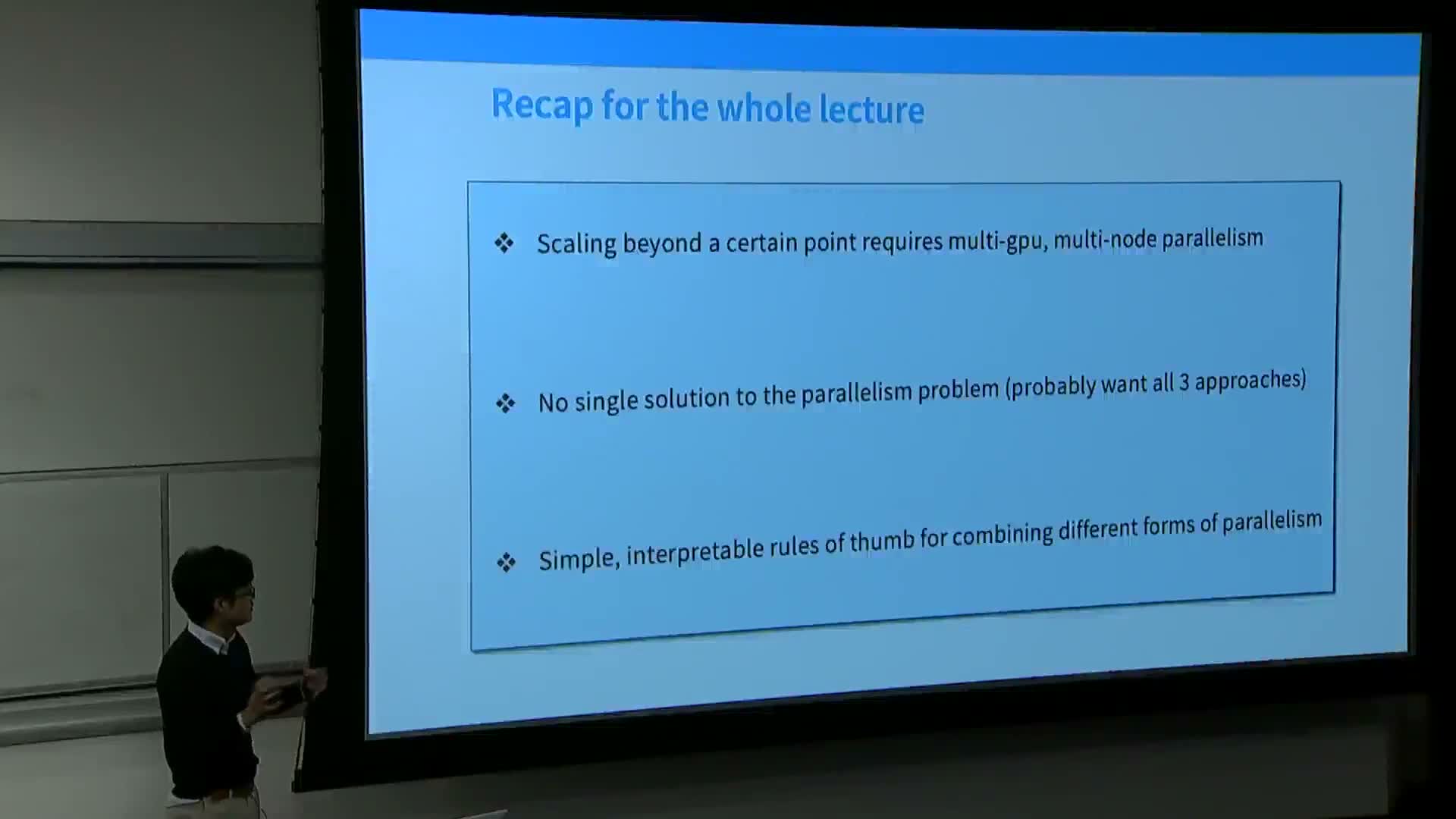
Practical summary and topology-aware heuristics:
- Combine data, model (tensor or pipeline), and activation (sequence) parallelism to balance limited resources—memory, bandwidth, compute, and batch size—while respecting hardware topology.
- Heuristics: apply tensor parallelism within nodes; use ZeRO/pipeline to fit models across nodes; scale throughput with data parallelism; use sequence/activation sharding and recomputation to minimize activation memory.
- Use gradient accumulation to trade time for larger effective batch sizes when necessary.
- Implementation notes: careful overlap of communication and computation plus attention to operational robustness enable near-linear aggregate throughput in practice.
Enjoy Reading This Article?
Here are some more articles you might like to read next: