CS336 Lecture 9 - Scaling laws
- Scaling laws provide a predictive framework for extrapolating small-model experiments to guide large-model design
- Scaling laws aim to produce simple, predictive relationships between model resources (data, parameters, compute) and model performance
- Scaling laws connect to classical statistical learning theory but operate on empirical realized losses rather than worst-case upper bounds
- Early empirical scaling-law thinking predates modern deep learning and proposed fitting predictive performance curves to avoid full-scale training
- Empirical neural scaling laws exhibit three phases—random/initial, power-law scaling, and asymptotic irreducible error—and are surprisingly predictive across domains
- Scaling behavior can break down for out-of-distribution or narrowly defined failure modes, producing non-scaling or inverse-scaling phenomena
- Large language model scaling exhibits consistent log-log linear relationships across compute, data, and parameters when measured in appropriate regimes
- Data-scaling laws map dataset size n to excess error and typically show log-log linear (power-law) decay in the productive regime
- Simple parametric estimation tasks yield power-law rates (e.g., mean estimation scales as 1/n) while nonparametric function estimation introduces intrinsic-dimension-dependent slower rates
- Observed empirical exponents for language-related tasks are often much smaller than simple parametric rates, reflecting high intrinsic complexity
- Generating synthetic data with controlled intrinsic dimensionality is straightforward, but estimating real data intrinsic dimension is challenging
- Data-scaling laws enable practical engineering decisions such as dataset composition, optimal mixing, and assessing diminishing returns from repetitions
- When analyzing data-scaling behavior, the model size used for evaluation must be large enough to avoid parameter-limited saturation
- Model-scaling analysis addresses trade-offs among architectures, optimizers, hyperparameters, and resource allocation for deployment
- Optimizer choice and depth/width/aspect-ratio choices can be evaluated via scaling curves to find scale-robust hyperparameter regimes
- Not all parameters are equivalent; embedding and sparsely activated parameters change scaling-law behavior and require normalization
- Batch size exhibits a critical threshold beyond which returns diminish, and the critical batch size itself scales with target loss
- Learning-rate optima vary with model width under standard parameterizations, but scale-stable reparameterizations (e.g., μP/new-p) can make the optimal learning rate transfer across widths
- Batch size and learning rate interact via gradient-noise considerations, and their optimal pairing can change with loss targets and modality
- Log-loss (next-token prediction) scaling is robust and predictable, but downstream task scaling and capability emergence can be far less predictable
- Scaling-law-based design prescribes training small models across orders of magnitude, fitting scaling relationships, and extrapolating optimal hyperparameters and architectures to full scale
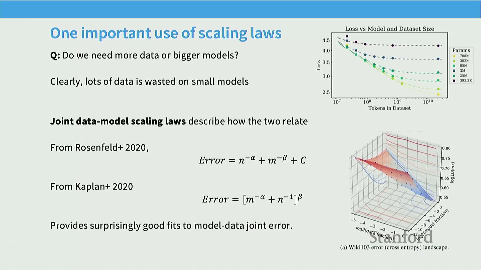
- Joint data–model scaling laws (iso-flop trade-offs) describe how loss decomposes into data-dependent and model-dependent components and enable optimal compute allocation
- The Chinchilla analysis operationalized iso-flop optimization and indicated an approximately 20 tokens-per-parameter budget under its assumptions
- Method 1 (minimum-envelope) finds the optimal model-size and data allocation by taking the lower envelope across many training curves
- Method 2 (isoflop analysis) finds the optimal parameter/data trade-off by minimizing loss along fixed-flop slices and reading out the minima
- Method 3 (direct joint functional fitting) fits a parametric two-variable surface to observed runs but requires careful regression to avoid biased coefficients
- Inference cost and deployment considerations have shifted preferred training regimes toward much higher tokens-per-parameter ratios
- Scaling-law methodologies generalize to different generative architectures (e.g., diffusion text models) and often reproduce similar iso-flop minima separated by constant offsets
- Log-linear scaling across data, parameters, and compute provides a unifying empirical foundation for many practical model-design and resource-allocation decisions
Scaling laws provide a predictive framework for extrapolating small-model experiments to guide large-model design

Scaling laws formalize using systematic small-scale experiments to predict the behavior of much larger models, reducing the compute and human cost of hyperparameter and architecture search.
-
Mechanism: train many small models across a range of sizes or compute budgets, fit simple functional forms to observed loss or metric trajectories, and extrapolate those fits to select configurations for a single large-scale run.
-
Rationale: avoid prohibitively expensive brute‑force tuning at full scale by relying on empirically validated extrapolations.
-
Implementation notes: ensure small-scale experiments cover the relevant regime (e.g., the power-law region) and use robust distributed training, data pipelines, and infra so extrapolation isn’t dominated by engineering artifacts.
This approach is especially useful in frontier labs where a single successful large-scale training run is the objective.
Scaling laws aim to produce simple, predictive relationships between model resources (data, parameters, compute) and model performance
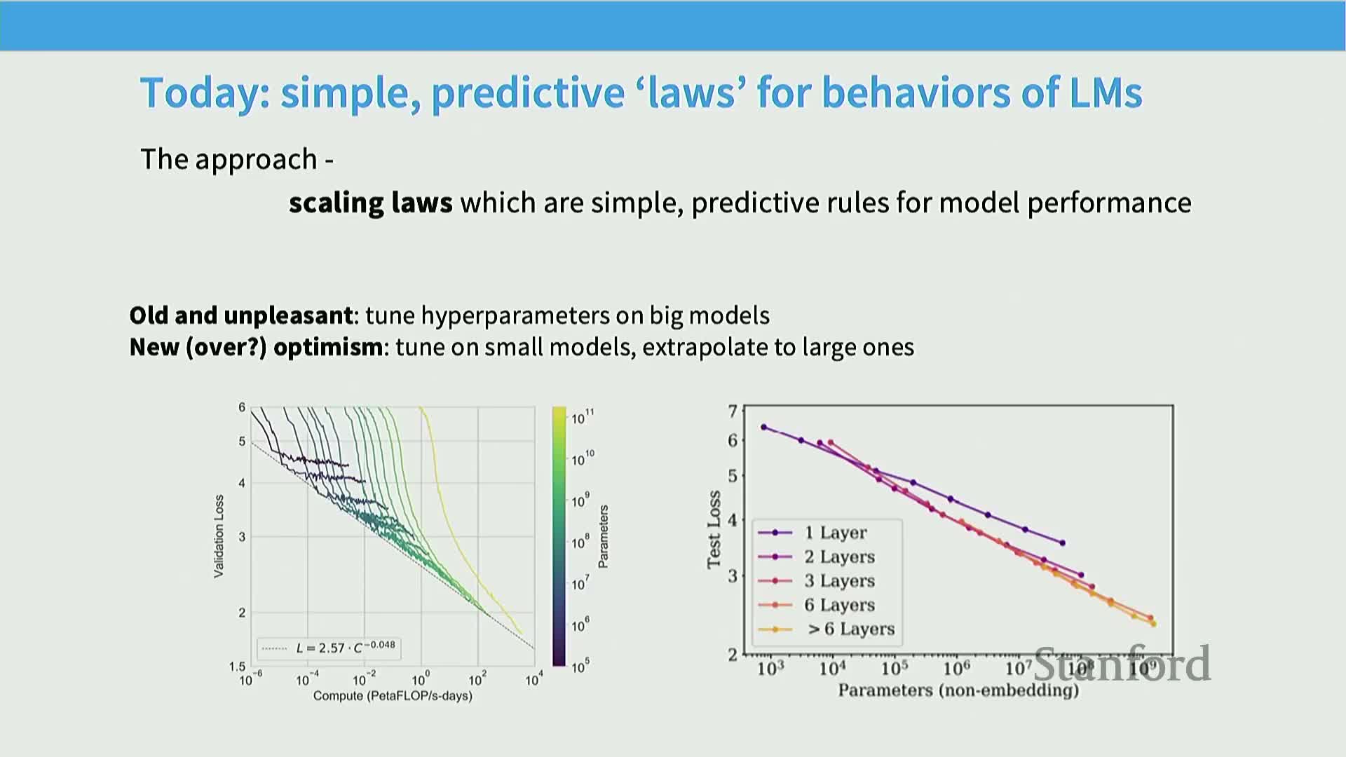
Scaling laws seek simple mathematical relationships that predict how performance metrics change when resources (dataset size, model parameters, compute) increase.
-
Central idea: fit compact empirical functions on small-scale runs and use them to make engineering decisions for larger runs.
-
Empirical regime: rely on monotonic, often approximately power-law dependencies where the model is not yet saturated by irreducible error.
-
Guidance produced: choices such as optimal parameter counts, data budgets, and compute allocations.
-
Practical requirement: choose resource ranges that avoid pathological regimes (random guessing or asymptotic irreducible error) so fitted forms are valid for extrapolation.
-
Program design: couple careful experimental design with regression or surface‑fitting techniques to quantify uncertainty in extrapolations.
Scaling laws connect to classical statistical learning theory but operate on empirical realized losses rather than worst-case upper bounds
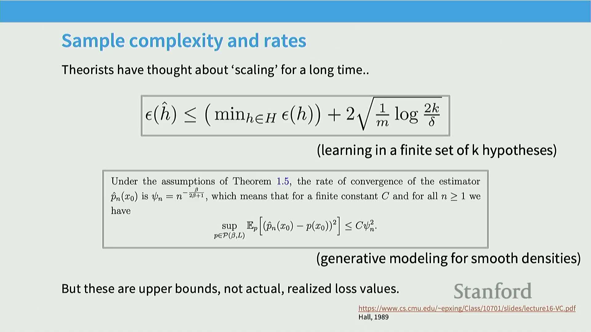
Classical theory (VC dimension, Rademacher complexity, nonparametric rates) gives asymptotic/worst-case bounds (e.g., O(1/√n) or n^{-β/(2β+1})) but these are upper bounds rather than observed loss trajectories.
-
Role of scaling laws: empirically fit functional relationships between dataset size, model capacity, and realized test loss to provide operational predictions for modern high-capacity models that violate simple theoretical assumptions.
-
Mechanism: treat empirical loss as the observable and use parametric or semi‑parametric curve fitting (e.g., power laws) across many runs to estimate exponents and offsets.
-
Rationale: empirical fits often deliver much tighter, actionable guidance than generic theory, especially for highly overparameterized neural networks.
-
Implementation considerations: carefully average over random seeds and use consistent evaluation metrics so fitted curves reflect true model behavior rather than noise.
Early empirical scaling-law thinking predates modern deep learning and proposed fitting predictive performance curves to avoid full-scale training
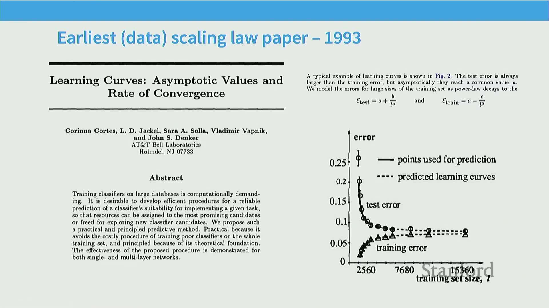
Work since the early 1990s proposed predicting classifier performance from partial or small-scale runs to select promising configurations without training full models.
-
Historical mechanism: decompose test error into irreducible error plus polynomially decaying terms, train many small models, fit decay curves (polynomial/power-law), and extrapolate to larger regimes — directly analogous to modern scaling-law practice.
-
Practical context: these historical results validate that systematic small-scale experiments can guide large-scale decisions and that power-law‑like fits often capture dominant behavior in the productive regime.
-
Implementation note: validate fitted functional forms against held-out experiments to avoid overconfident or biased extrapolation.
Empirical neural scaling laws exhibit three phases—random/initial, power-law scaling, and asymptotic irreducible error—and are surprisingly predictive across domains
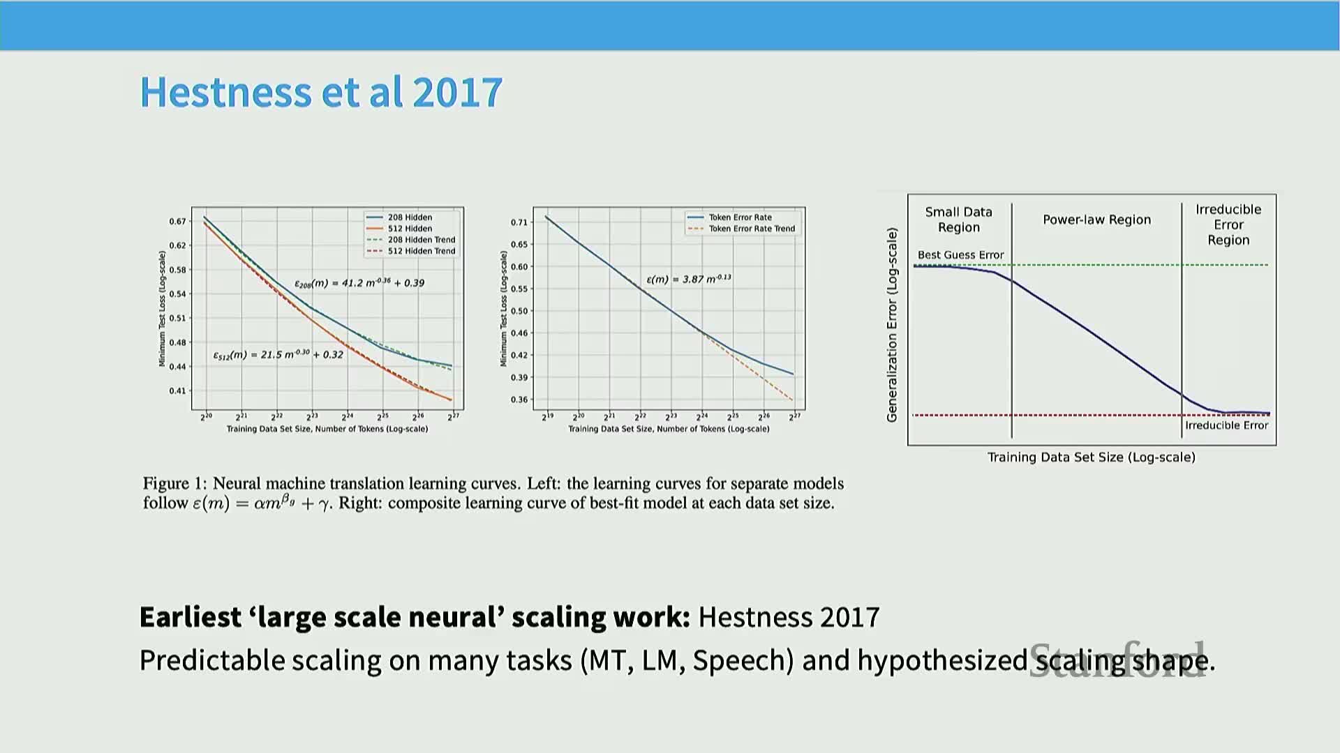
Empirical studies across translation, speech, and vision identify a characteristic three‑phase curve shape for loss versus resources:
-
Initial region near random performance — difficult to extrapolate.
-
Middle regime where loss decreases approximately as a power law with resources — the predictive domain for scaling laws.
-
Asymptotic region approaching irreducible error where gains taper off and extrapolation is unreliable.
-
Mechanistic insight: scaling-law procedures restrict fits to the intermediate regime where predictions are most reliable.
-
Practical implication: design experiments to avoid model saturation so the middle regime is well sampled.
-
Robustness: this three‑phase behavior appears across architectures and tasks and underpins confidence that small-scale experiments can inform large-scale outcomes when the right regime is targeted.
Scaling behavior can break down for out-of-distribution or narrowly defined failure modes, producing non-scaling or inverse-scaling phenomena
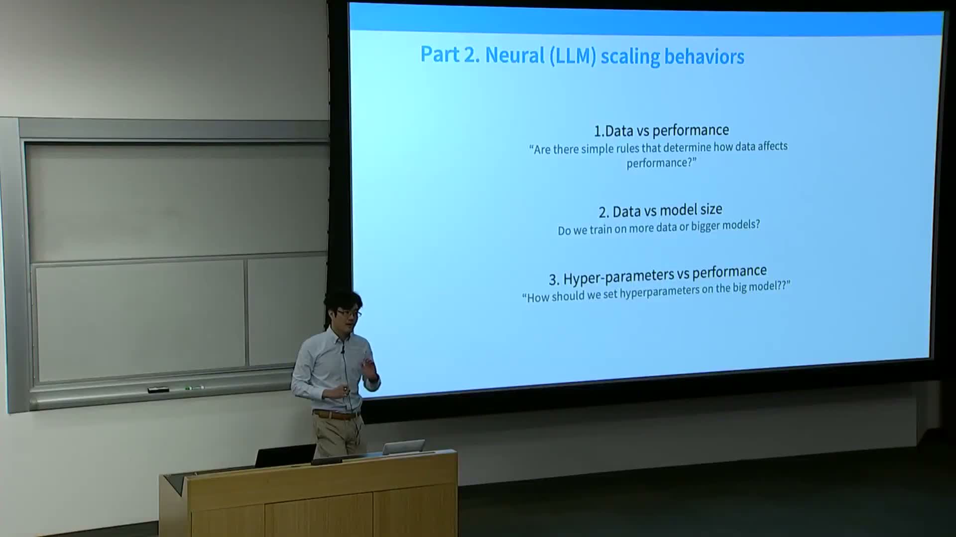
Scaling is natural for metrics like held-out training loss because improvement is typically monotonic with more data or capacity, but some capabilities or pathological behaviors can degrade with scale.
-
Examples: tasks from inverse-scaling studies where certain capabilities become worse as models grow, or where extreme out‑of‑distribution (OOD) performance does not improve monotonically.
-
Mechanism for non-scaling: occurs when the evaluation domain drifts far from the training distribution or when tasks depend on brittle heuristics that do not benefit from capacity in conventional ways.
-
Practical implication: extrapolation must be task-aware — don’t assume universal log‑log linearity for all downstream behaviors; directly measure the phenomenon of interest across scale to verify the assumed scaling.
Large language model scaling exhibits consistent log-log linear relationships across compute, data, and parameters when measured in appropriate regimes
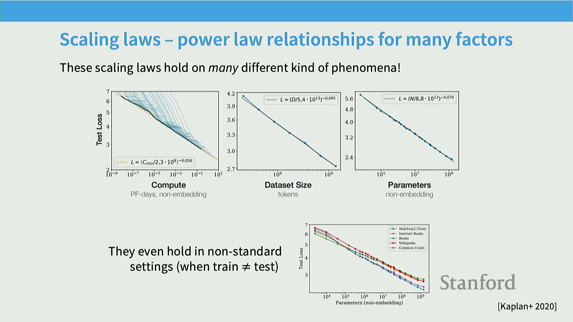
When evaluated on next-token prediction or other log‑loss metrics in the middle power‑law regime, models show approximately linear trends on log‑log plots between resource axes (compute, data, parameters) and test loss.
-
Empirical mechanism: hold one resource large enough to avoid saturation and vary the other to reveal the power‑law region (e.g., keep model size large while varying data to study data scaling).
-
Rationale: log‑log linearity (power laws) is a compact functional form that fits many empirical curves, enabling interpolation and extrapolation across orders of magnitude.
-
Implementation caveat: ensure the held‑constant resource is actually large enough and that evaluation is done in a regime where the power‑law model is valid before extrapolating.
Data-scaling laws map dataset size n to excess error and typically show log-log linear (power-law) decay in the productive regime
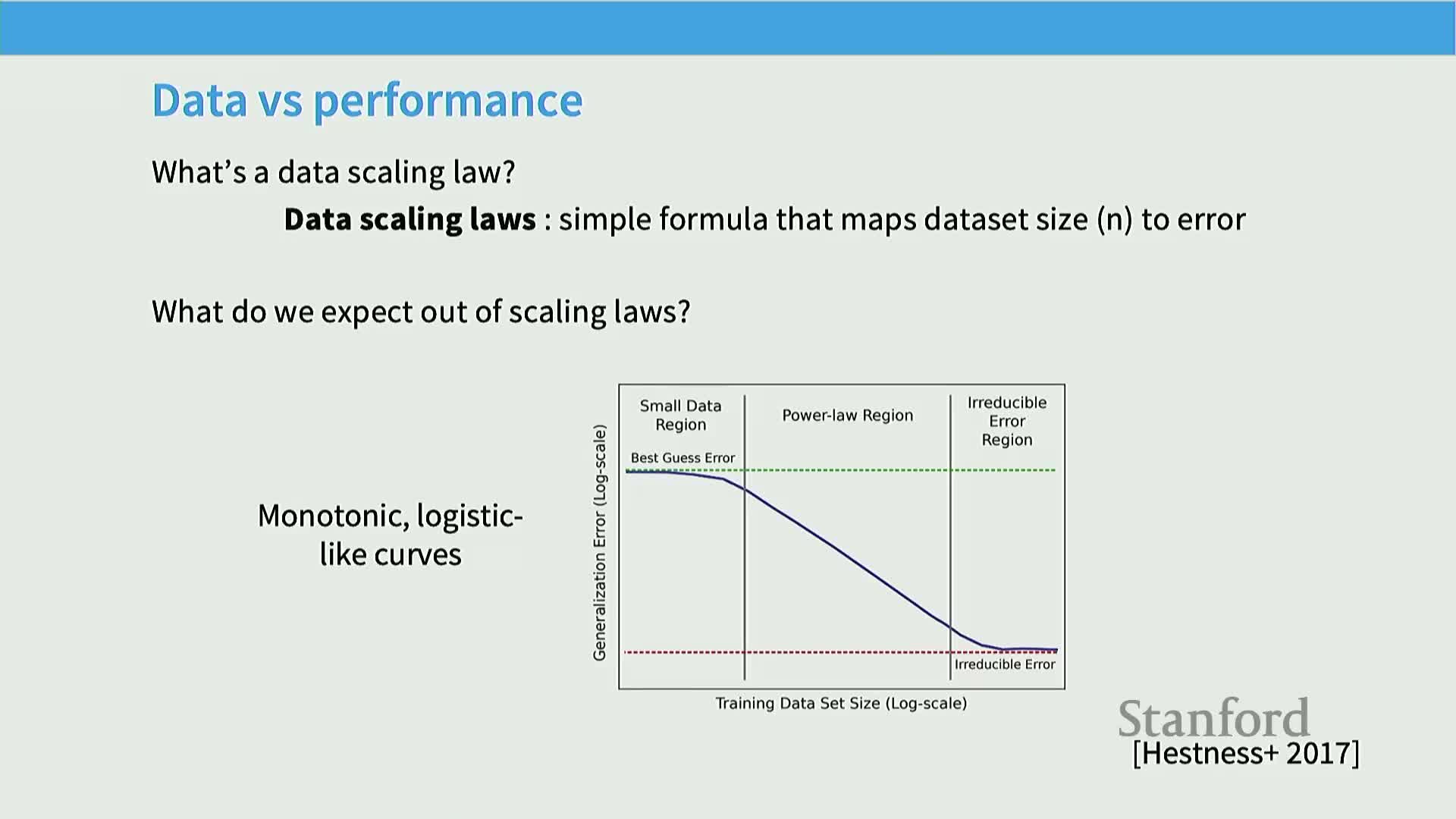
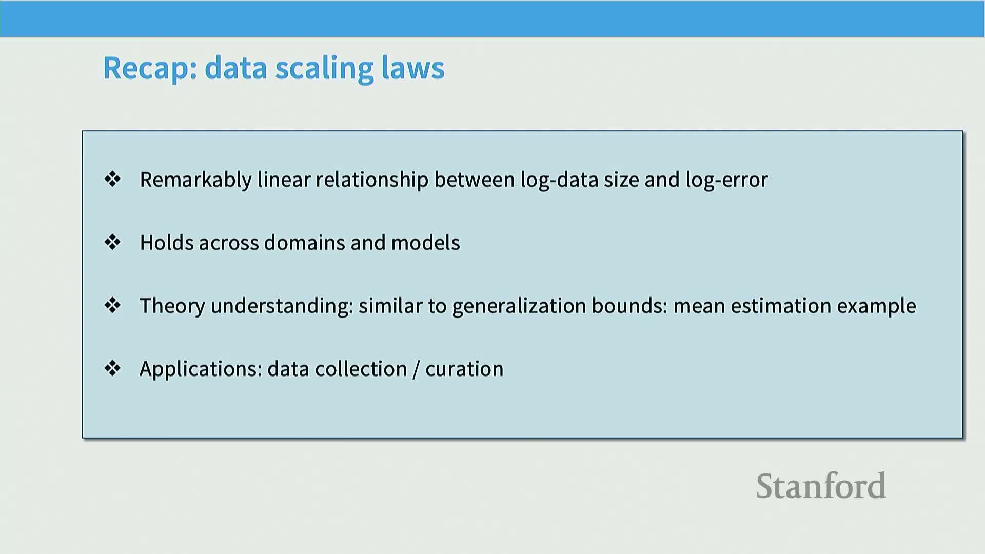
Data‑scaling analysis focuses on the excess error (error above irreducible noise) as a function of the number of unique training tokens n and often finds error ∝ n^{-α} in the power‑law regime.
-
Mechanism: train models with fixed high capacity while varying dataset sizes, plot test loss versus n on log‑log axes, and fit a straight line to estimate the exponent α.
-
Rationale: identifying α and the offset enables predictions about how much additional data is needed to achieve a target reduction in loss and supports tradeoffs like data collection vs. compute allocation.
-
Implementation notes: focus on unique‑token counts (account for repeated‑epoch effects separately) and validate that the fitted exponent is stable across model sizes within the power‑law region.
Simple parametric estimation tasks yield power-law rates (e.g., mean estimation scales as 1/n) while nonparametric function estimation introduces intrinsic-dimension-dependent slower rates
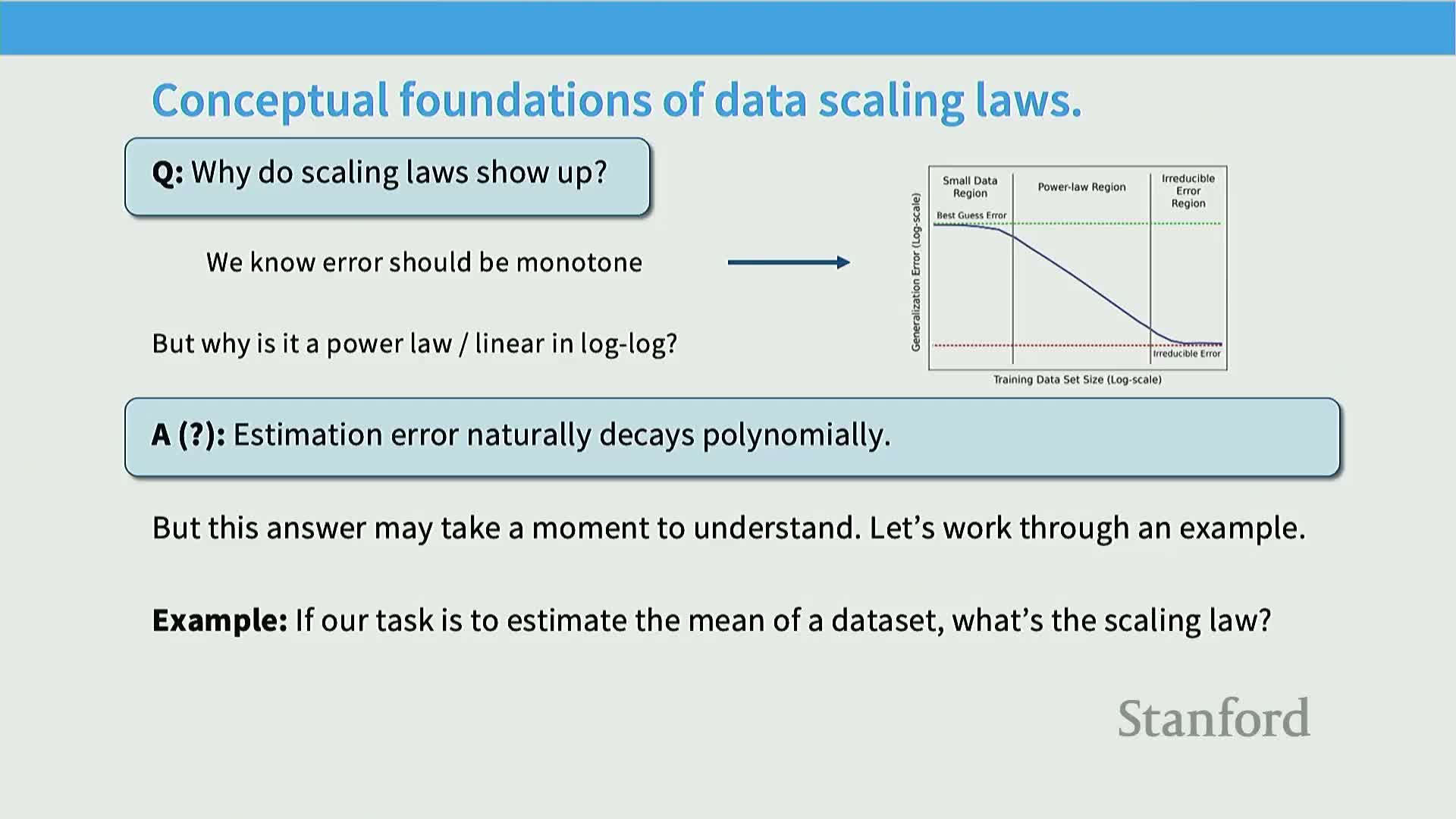
Elementary tasks explain why polynomial decay in n is natural:
-
Gaussian mean estimation: mean‑squared error ∝ σ^2/n, so log‑error is linear in log n with slope −1.
-
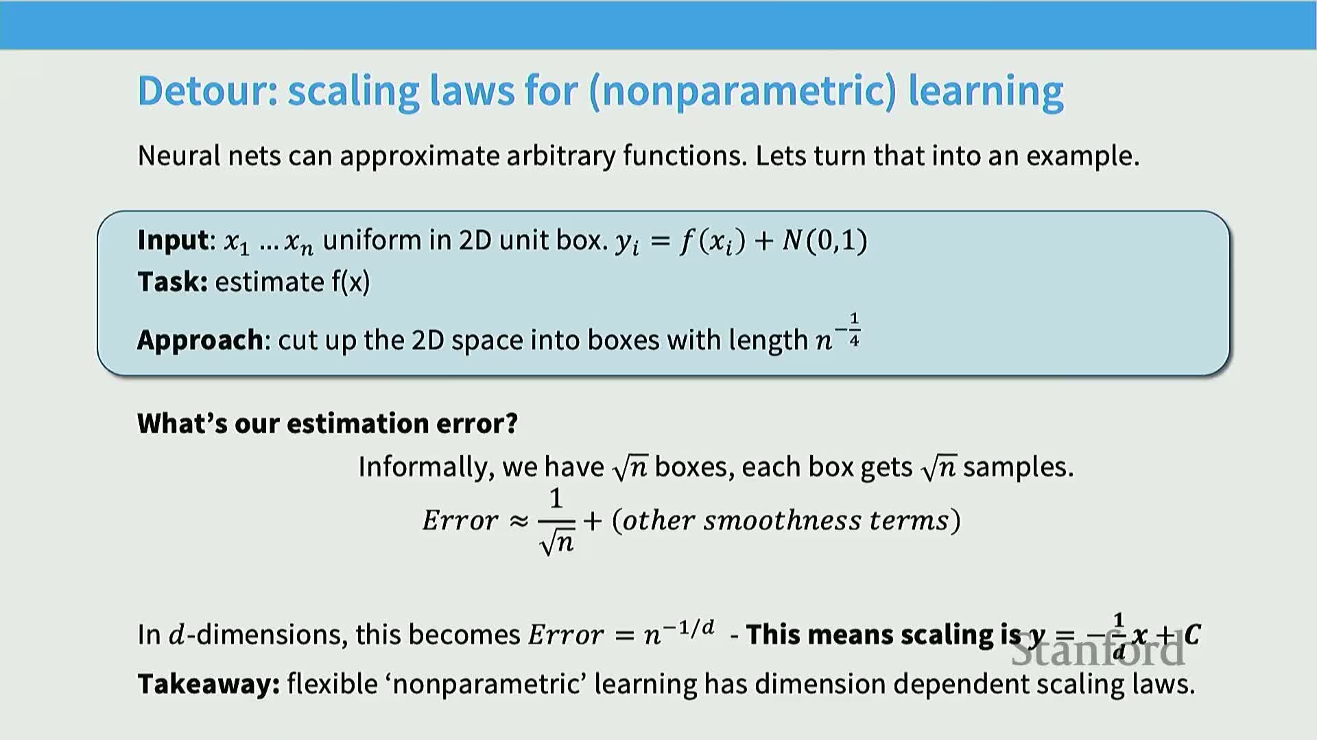
Nonparametric regression: covering input domain with bins yields error scaling like n^{-1/d} for data uniformly distributed in d dimensions; effective learning rate decays more slowly as intrinsic dimension increases.
-
Mechanistic takeaway: flexible function classes require exponentially more samples to resolve fine structure in higher intrinsic dimensions, reflected as smaller exponents on log‑log error plots.
-
Rationale: shallow exponents in language modeling can be understood as consequences of high intrinsic dimensionality; inducing strong inductive biases or estimating intrinsic dimension can change the empirical exponent.
-
Implementation caveat: intrinsic dimension is hard to estimate robustly, so interpret exponents cautiously and validate across datasets and architectures.
Observed empirical exponents for language-related tasks are often much smaller than simple parametric rates, reflecting high intrinsic complexity
Empirical studies report exponents substantially below classical parametric expectations (examples: ~0.13 for MT, ~0.3 for speech, and ≈0.95 in some LM settings), meaning errors decline much more slowly with dataset size than naive 1/n or 1/√n rates.
-
Mechanism: modern language and speech tasks involve highly nonparametric target functions with large effective dimensionality and complex structure, increasing sample complexity.
-
Rationale: shallow empirical exponents imply enormous increases in tokens are needed for modest loss gains, motivating strategies that optimize model architecture and data mixtures rather than naive data accumulation.
-
Implementation note: estimate empirical exponents using a broad range of dataset sizes and carefully control confounders such as model capacity and evaluation protocol.
Generating synthetic data with controlled intrinsic dimensionality is straightforward, but estimating real data intrinsic dimension is challenging
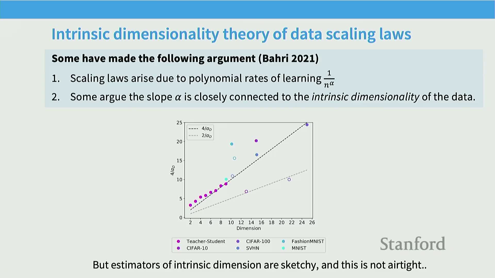
To create data with a chosen intrinsic dimension for experiments, specify a function of k latent variables plus noise to produce manifolds of known dimension.
-
Mechanism: synthetic manifolds validate predicted n^{-1/d} behavior in nonparametric estimation.
-
Practical implication: synthetic experiments are useful for theory validation, but translating results to complex real data (code, natural text) requires caution because true generative factors and interactions are unknown and noisy.
-
Implementation note: use additional empirical diagnostics when moving from synthetic to real‑world corpora.
Data-scaling laws enable practical engineering decisions such as dataset composition, optimal mixing, and assessing diminishing returns from repetitions
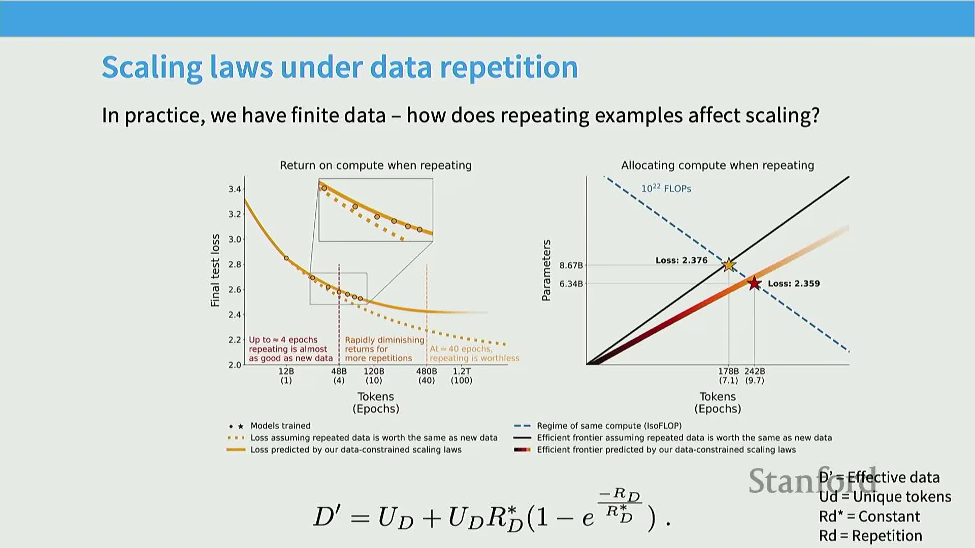
Scaling‑law fits can quantify how dataset composition shifts the loss offset without substantially changing the exponent, enabling evaluation of relative data‑quality decisions on smaller models and extrapolation to large regimes.
-
Mechanism: fit scaling laws per data source and estimate their contributions to mixed‑data performance, enabling regression‑based optimal mixing strategies for trillion‑token regimes.
-
Extension: scaling laws extend to multi‑epoch training by defining an effective unique‑token count that diminishes with repetition, helping decide whether to repeat high‑quality data or add lower‑quality new data.
-
Implementation caveats: data‑selection research is empirically difficult; validate that per‑mixture power‑law assumptions hold in the target regime.
When analyzing data-scaling behavior, the model size used for evaluation must be large enough to avoid parameter-limited saturation
Data‑scaling experiments assume the model is not the bottleneck; therefore experimenters select model sizes sufficiently larger than the task’s effective complexity so loss is dominated by data scarcity rather than model capacity.
-
Mechanic: keep model parameters high and vary only dataset size when fitting data‑scaling exponents.
-
Rationale: if the model is saturated, fitted data‑scaling laws will reflect model limitations rather than true data‑driven gains, invalidating extrapolations.
-
Implementation note: when presenting data‑scaling plots, document the fixed model size and verify that increasing the model further does not substantially change the fitted exponent in the regime of interest.
Model-scaling analysis addresses trade-offs among architectures, optimizers, hyperparameters, and resource allocation for deployment
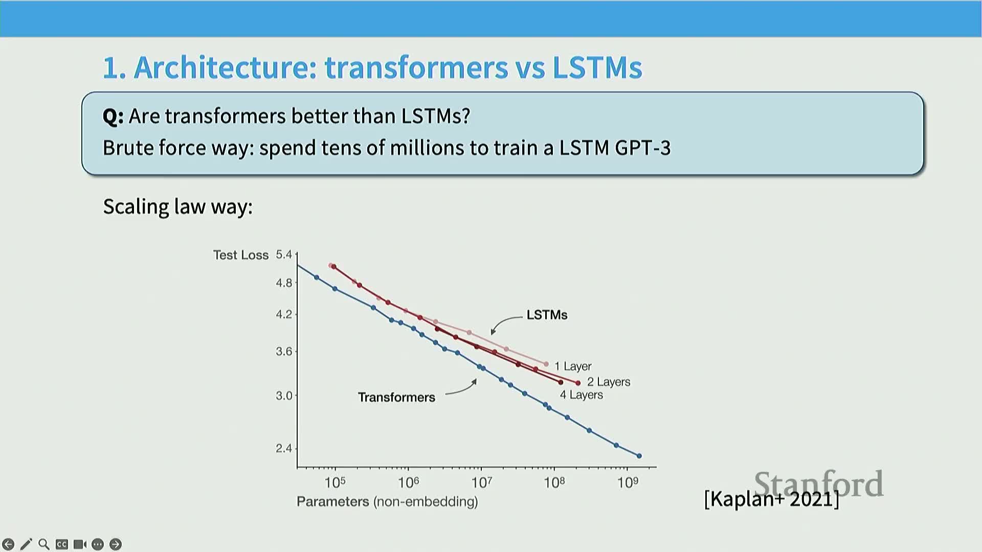
Model‑scaling law methodology evaluates architectures (transformers, LSTMs, state‑space models, gated units, MoE), optimizers (SGD, Adam), and hyperparameters by training families of models across compute budgets and comparing their loss‑versus‑compute trajectories.
-
Mechanistic pattern: curves for different architectures often appear as non‑crossing, parallel‑like lines on log‑log plots, indicating constant‑factor compute efficiency differences and enabling extrapolation that lower‑offset architectures perform better across scales.
-
Rationale: reveals which innovations are worth scaling (e.g., gated linear units, mixture‑of‑experts) and which provide limited benefit when compute is abundant.
-
Implementation considerations: account for parameter types (embeddings vs. non‑embedding parameters) and normalize sparse/conditional parameterizations into equivalent dense‑parameter measures for fair comparisons.
Optimizer choice and depth/width/aspect-ratio choices can be evaluated via scaling curves to find scale-robust hyperparameter regimes
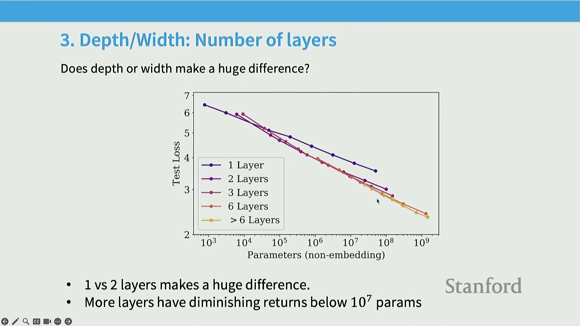
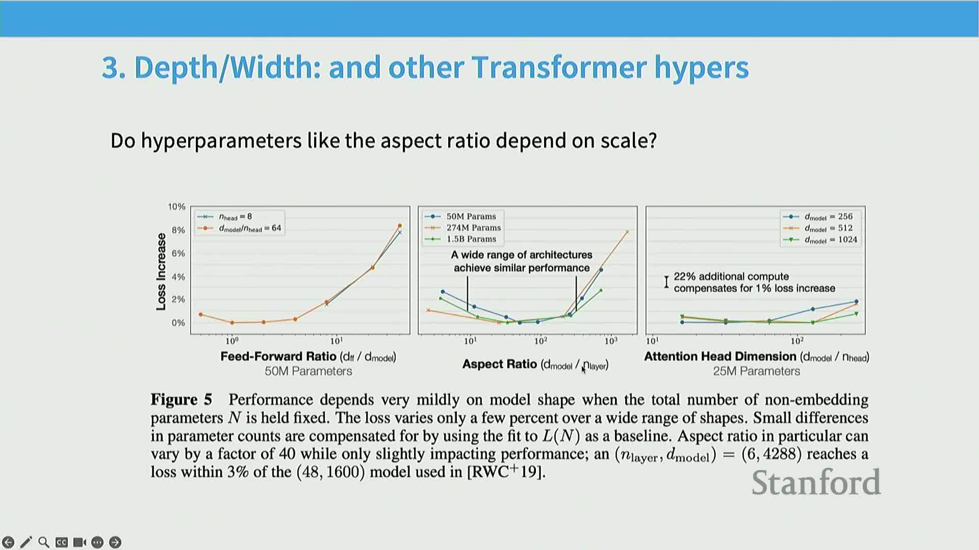
Scaling studies comparing optimizers show approximately constant‑factor differences in compute efficiency across dataset sizes, and depth‑versus‑width sweeps reveal broad basins of near‑optimal aspect ratios rather than sharp optima.
-
Mechanism: train many models at multiple sizes and plot loss versus compute to test whether slopes and offsets of scaling curves vary across hyperparameter choices; conserved slopes with differing offsets imply small‑scale tuning can transfer to large scale.
-
Rationale: scaling‑law sweeps avoid repeated costly retuning at each scale and identify hyperparameter settings robust across sizes.
-
Implementation notes: sweep multiple sizes (e.g., 50M, 270M, 1.5B) and fit surfaces or envelopes to identify consistent minima.
Not all parameters are equivalent; embedding and sparsely activated parameters change scaling-law behavior and require normalization
Certain parameter classes (e.g., embedding tables) do not participate in scaling the same way as non‑embedding transformer parameters, producing bends or deviations in naive parameter‑versus‑loss curves.
-
Mechanism: counting embeddings as ordinary parameters can distort fitted exponents and offsets, so analyses either exclude embeddings or convert sparse/specialized parameters into an equivalent dense‑parameter metric.
-
For conditional/sparse architectures (MoE): derive an equivalent dense‑parameter count to enable fair comparisons and meaningful scaling predictions.
-
Implementation implication: reports should specify which parameter subsets were counted and how sparsity/activation patterns were normalized for cross‑architecture scaling comparisons.
Batch size exhibits a critical threshold beyond which returns diminish, and the critical batch size itself scales with target loss
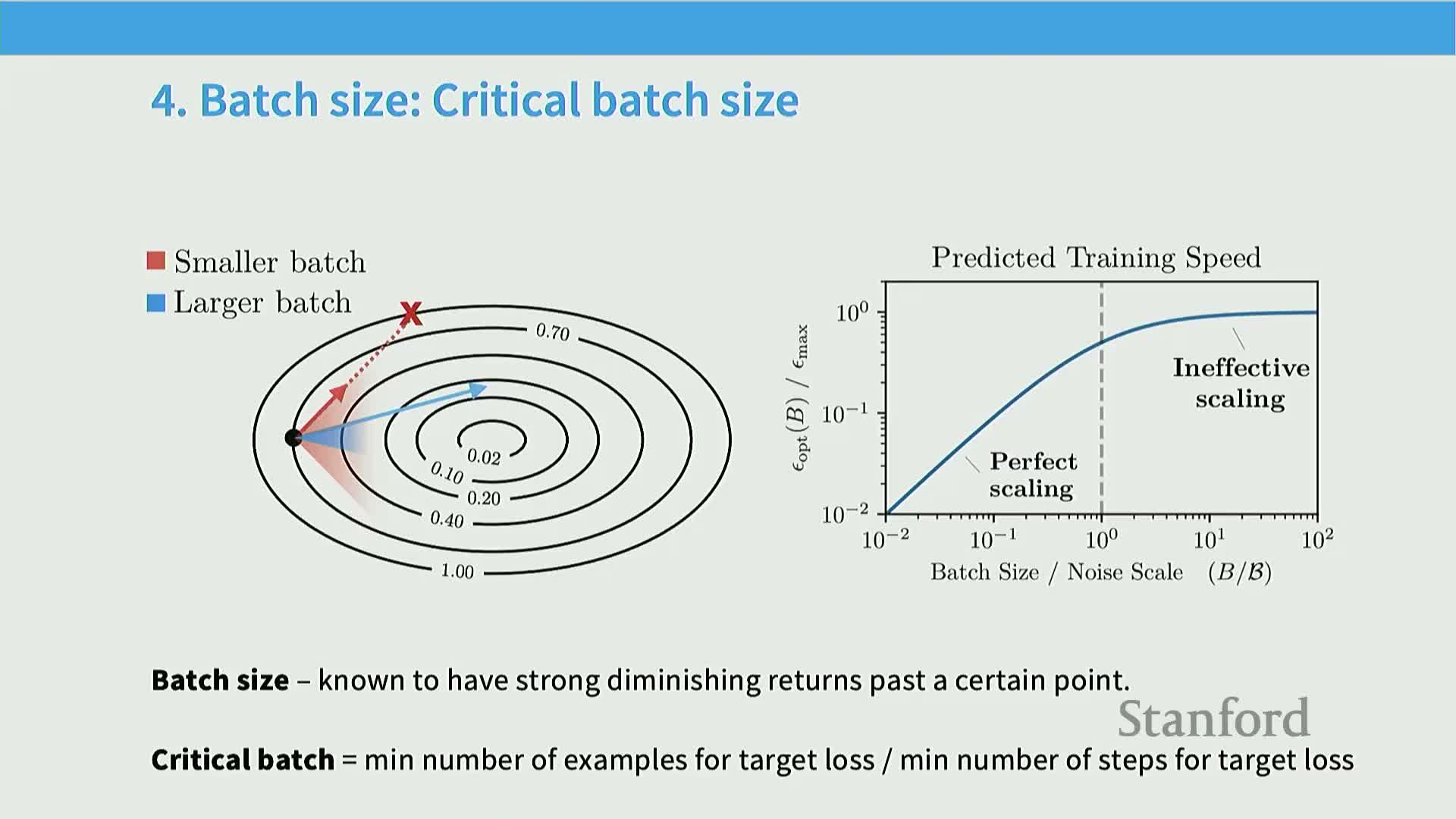
Increasing batch size up to the gradient‑noise scale yields near‑linear wall‑clock/step equivalence (doubling batch size ≈ taking two gradient steps) and is therefore an effective systems optimization; past a critical batch size, additional samples per step stop reducing stochastic gradient noise and yield diminishing returns.
-
Mechanism: the noise scale defines the regime boundary where optimization transitions from noise‑dominated to curvature‑dominated; the critical batch size can be estimated empirically or modeled theoretically.
-
Empirical observation: the critical batch size tends to decrease as the target loss becomes smaller, so schedules and parallelization should adapt during training.
-
Implementation consequences: plan batch‑size schedules and balance data‑parallel throughput with optimization efficiency; many large training reports adjust batch sizes during runs.
Learning-rate optima vary with model width under standard parameterizations, but scale-stable reparameterizations (e.g., μP/new-p) can make the optimal learning rate transfer across widths
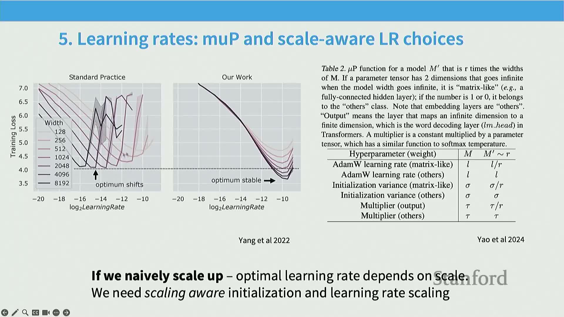
Under conventional transformer parameterizations the optimal learning rate typically decreases as width increases, producing different tuned optima at different scales and complicating hyperparameter transfer from small to large models.
-
Mechanism: reparameterizations that scale initializations and layer‑wise update magnitudes as a function of width (e.g., μP or variants) normalize the optimization landscape so a single learning‑rate choice tuned at small scale remains near‑optimal at larger widths.
-
Rationale: scale‑stable parameterizations reduce the need for repeated learning‑rate sweeps across model sizes and simplify large‑scale training planning.
-
Implementation caveat: μP‑like schemes improve transferability but are not a panacea; multiple variants exist (e.g., Meta’s metap) and require empirical validation in each training stack.
Batch size and learning rate interact via gradient-noise considerations, and their optimal pairing can change with loss targets and modality
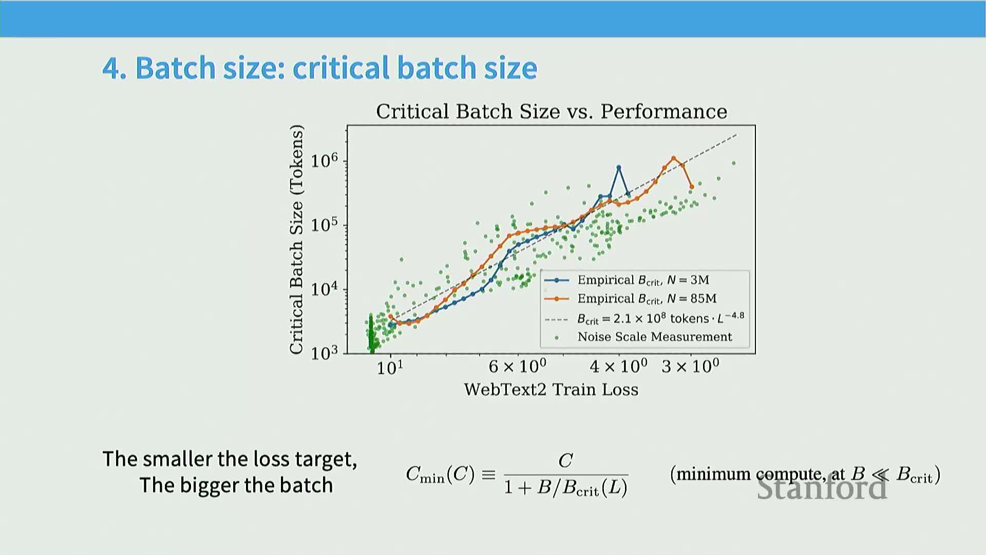
Optimal batch‑size choices are linked to noise scale and learning‑rate schedules; as training progresses toward lower loss targets, practitioners often increase batch size to reduce gradient noise that would otherwise force smaller learning rates or conservative updates.
-
Mechanism: batch size and learning rate affect gradient variance and step size in opposing ways, so their joint tuning is necessary for stable large‑scale training.
-
Practical considerations: modality‑specific behavior (NLP vs. vision) matters and noise‑scale theory gives qualitative guidance rather than a universal prescription.
-
Implementation advice: empirically estimate critical batch sizes and validate learning‑rate transfer or reparameterization choices for the specific model and dataset.
Log-loss (next-token prediction) scaling is robust and predictable, but downstream task scaling and capability emergence can be far less predictable
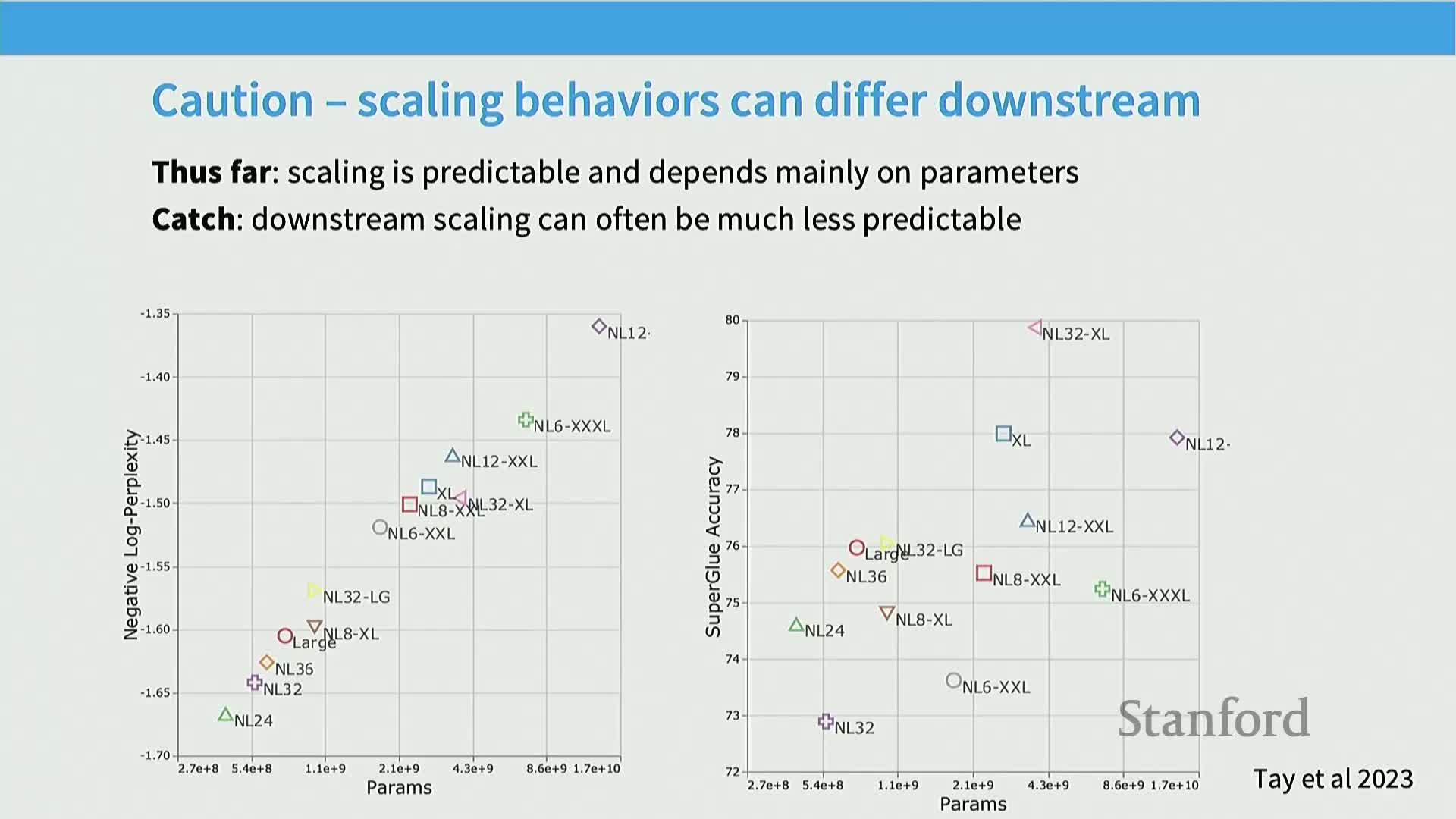
Cross‑entropy or negative log‑likelihood scales smoothly and is highly amenable to log‑log linear modeling across architectures and compute levels, explaining why many scaling‑law results focus on perplexity or test loss.
-
Mechanism for mismatch: mapping log‑loss improvements to downstream benchmarks (accuracy, QA, in‑context learning) is often nonlinear and can vary widely across architectures and hyperparameters because task capabilities depend on subtle behaviors not fully captured by perplexity.
-
Practical implication: use direct empirical evaluation on the downstream task of interest rather than assuming that perplexity scaling automatically translates to better task performance.
Scaling-law-based design prescribes training small models across orders of magnitude, fitting scaling relationships, and extrapolating optimal hyperparameters and architectures to full scale
Practical recipe for using scaling laws:
- Run small‑to‑medium scale experiments spanning multiple orders of magnitude in compute.
- Verify loss versus resource relationships show stable log‑log linearity (or another valid functional form).
- Fit relationships to extract slopes and offsets.
- Use fits to choose model size, data budget, batch size, and hyperparameters for a single large‑scale run.
-
Mechanism: relies on conserved slopes (non‑crossing curves) so small‑scale minima and offsets transfer to larger scales.
-
Rationale: reduces risk and cost compared to brute‑force large‑scale hyperparameter searches.
-
Caveats: some parameters (e.g., learning rate) may not transfer without reparameterization.
-
Best practices: span a broad compute range, report fit uncertainty, and validate extrapolations with a limited number of larger intermediate runs when feasible.
Joint data–model scaling laws (iso-flop trade-offs) describe how loss decomposes into data-dependent and model-dependent components and enable optimal compute allocation
Joint scaling models posit additive or multiplicative decompositions of error into terms that decay polynomially with data (n) and model size (m), plus irreducible error, often written as Loss(n,m) ≈ c_n n^{-α_n} + c_m m^{-α_m} + c_0.
-
Mechanism: fit such a two‑variable surface across grids of (n,m) to compute iso‑flop curves that show optimal parameter/token trade‑offs for a fixed compute budget.
-
Rationale: answer whether to allocate compute to more parameters or more data and derive prescriptions (e.g., tokens‑per‑parameter ratios) that minimize loss for fixed flops.
-
Implementation notes: perform careful surface fitting, account for learning‑rate and schedule interactions, and validate extrapolations with held‑out larger‑scale runs.
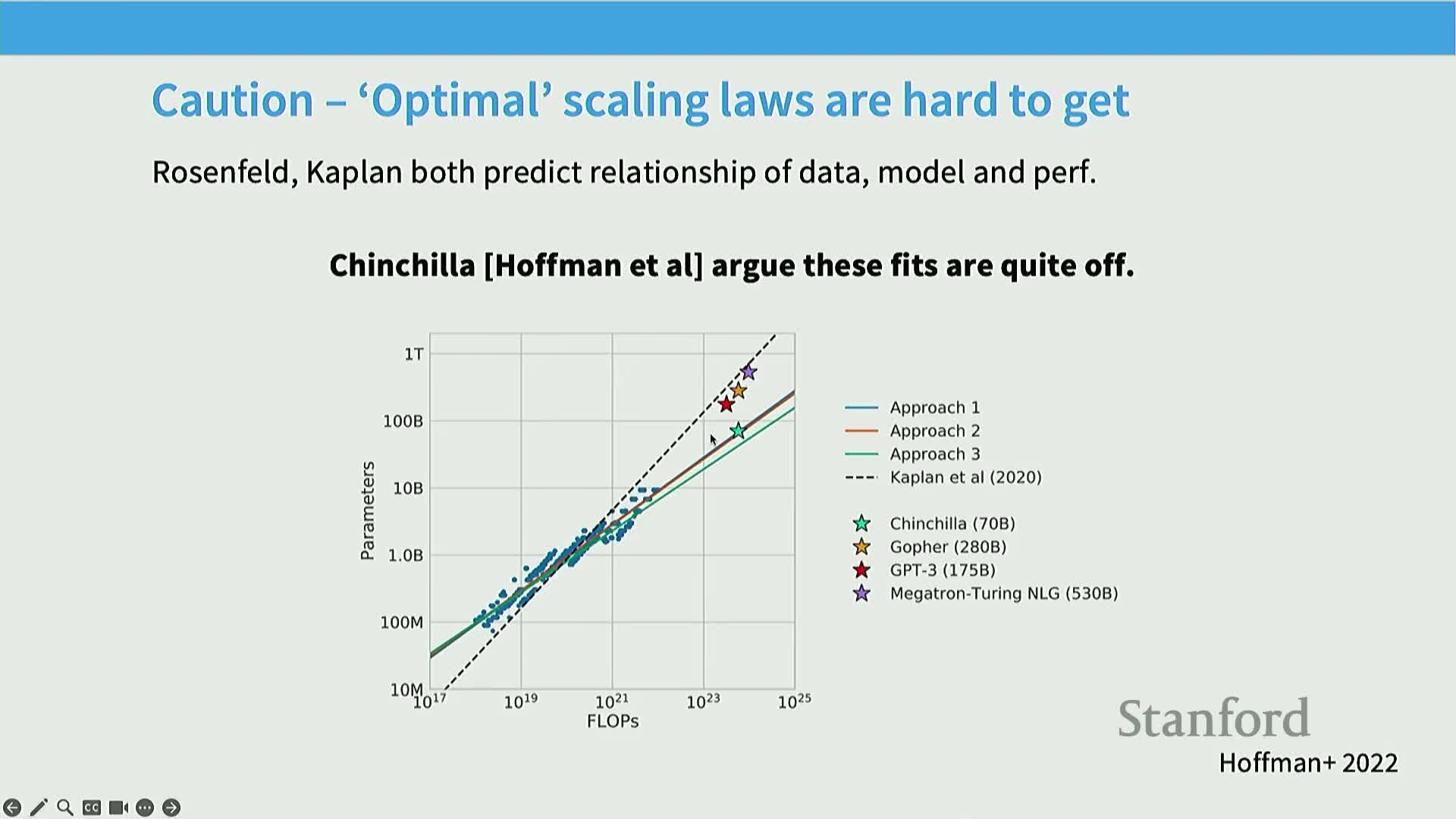
The Chinchilla analysis operationalized iso-flop optimization and indicated an approximately 20 tokens-per-parameter budget under its assumptions
Chinchilla used three empirical methods to infer the optimal token‑to‑parameter ratio for minimizing loss at fixed training flops and found a consistent recommendation near ~20 tokens per parameter under their training protocol and schedules.
-
Mechanisms used: lower envelope of performance across models, isoflop minima extraction via quadratic fits per compute slice, and direct joint functional form fitting; the first two produced similar coefficients while the third required careful regression handling.
-
Rationale: the tokens‑per‑parameter guideline provided a practical balance between parameter count and dataset size for a given compute budget and guided many subsequent training budgets.
-
Implementation caveat: the precise optimal ratio depends on learning‑rate schedule, optimization details, and evaluation protocol, so reproducing the exact number requires matching training recipes.
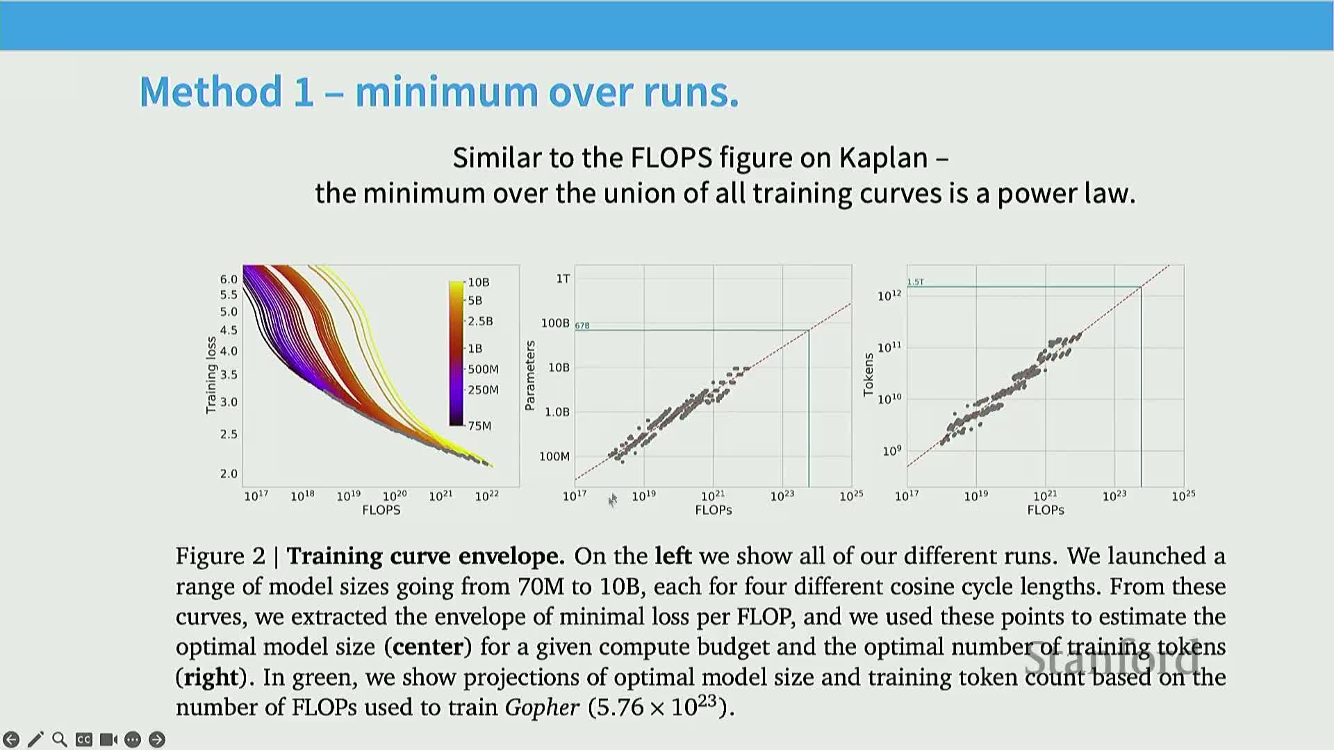
Method 1 (minimum-envelope) finds the optimal model-size and data allocation by taking the lower envelope across many training curves
The minimum‑envelope method overlays training curves for models of different parameter counts across compute budgets and selects the lower envelope of achievable loss for each compute level.
-
Mechanism: read off the parameter count and token count at the envelope to get an empirical optimal token‑to‑parameter ratio; the approach is nonparametric and leverages the smooth curve formed by observed optima.
-
Rationale: makes minimal modeling assumptions and directly uses observed optima, making it robust when grid coverage is sufficient.
-
Implementation requirements: train a dense grid of model sizes and checkpoints across compute so the envelope is well‑resolved; use interpolation or local quadratic fits to reduce noise when identifying minima.
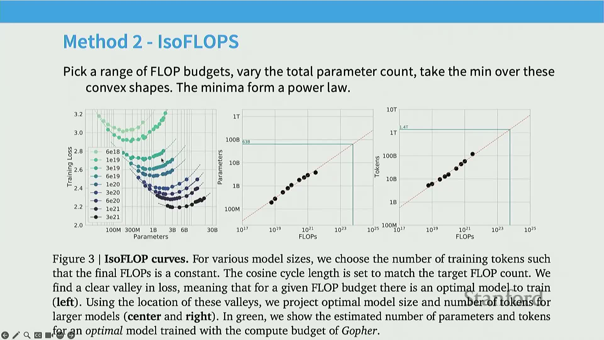
Method 2 (isoflop analysis) finds the optimal parameter/data trade-off by minimizing loss along fixed-flop slices and reading out the minima
Isoflop analysis fixes total compute (flops) and, for each compute level, sweeps model sizes and corresponding token counts to find the configuration that minimizes loss within that budget.
-
Mechanism: implement by fitting local quadratics to loss‑versus‑parameter curves at each isoflop and extracting minima to reduce measurement noise.
-
Rationale: directly answers how to allocate a given compute budget between model size and dataset size.
-
Implementation notes: require careful curve smoothing and validation across multiple compute levels to ensure minima form a stable power‑law curve amenable to extrapolation.
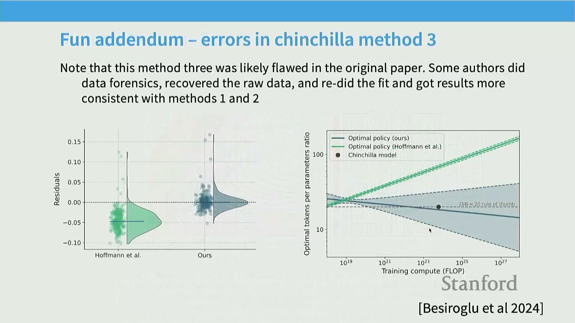
Method 3 (direct joint functional fitting) fits a parametric two-variable surface to observed runs but requires careful regression to avoid biased coefficients
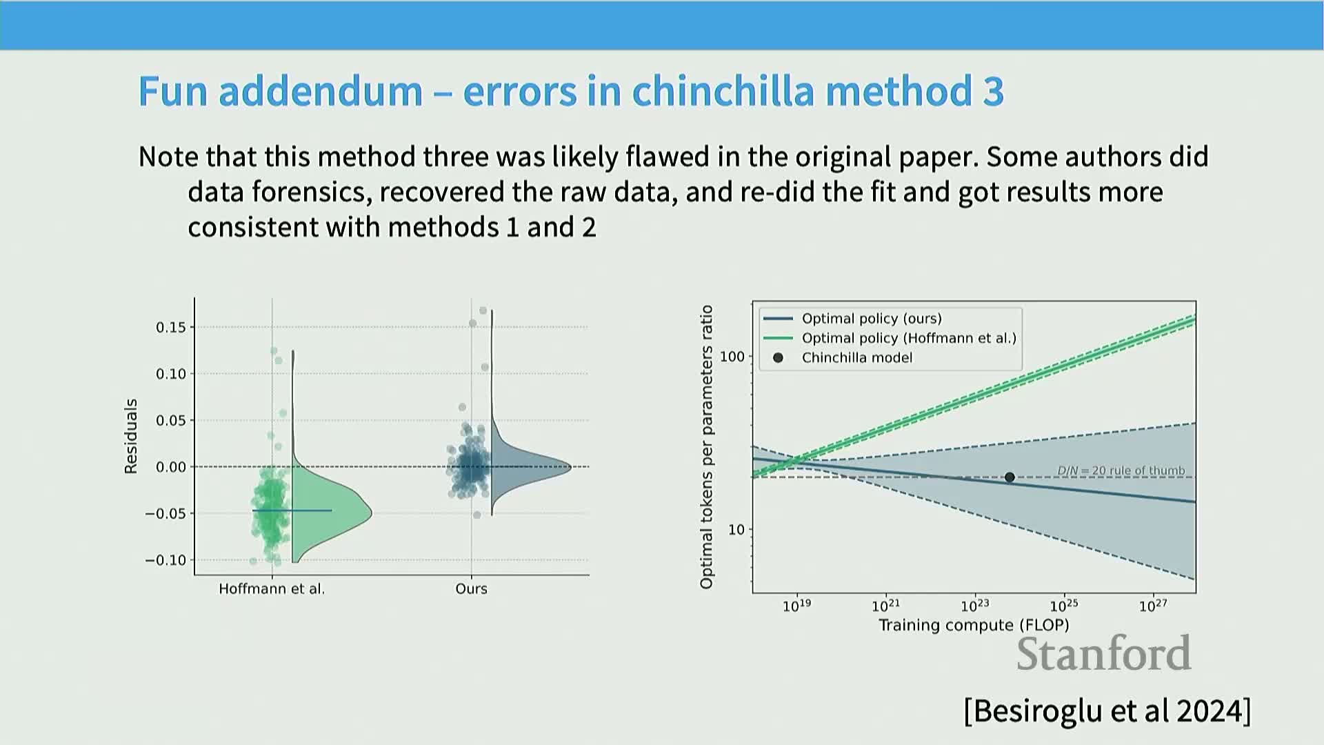
An alternative approach fits a global parametric form Loss(n,m)=c_n n^{-α_n}+c_m m^{-α_m}+c_0 to all observed runs and extracts optimal trade‑offs from the fitted surface.
-
Mechanistic risk: sensitive to regression setup and residual structure; non‑zero‑mean residuals or heteroscedasticity can bias estimated exponents and conflict with envelope or isoflop methods.
-
Empirical lesson: documented replication found that correcting residual issues reconciled the global fit with envelope/isoflop methods, highlighting the importance of statistically careful fitting.
-
Implementation takeaway: inspect residuals, consider weighted regression, and validate global fits against lower‑envelope or isoflop minima to ensure consistent conclusions.
Inference cost and deployment considerations have shifted preferred training regimes toward much higher tokens-per-parameter ratios
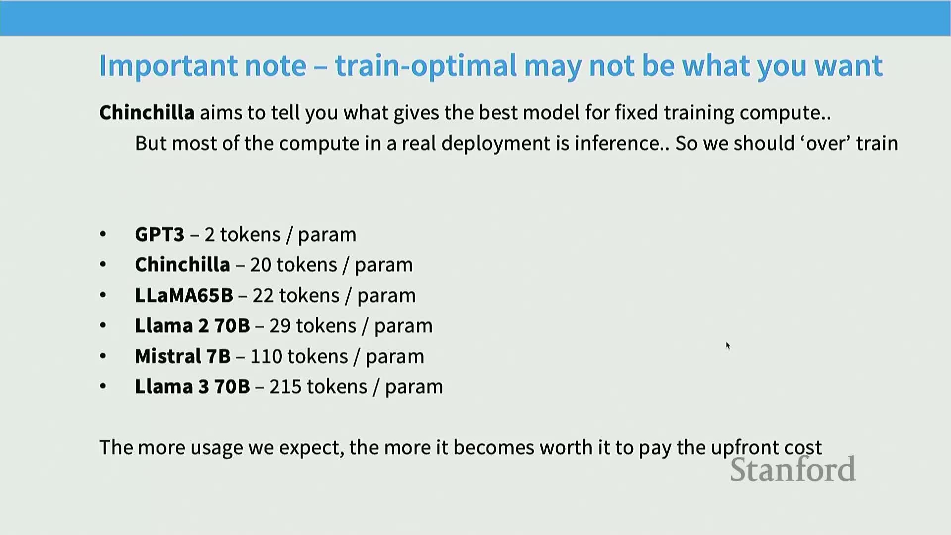
As models became deployed products with recurring inference costs, the operational trade‑off shifted: pay more one‑time training cost (increased tokens per parameter) to produce smaller models that are cheaper to serve at inference time.
-
Mechanism: increasing tokens per parameter while reducing parameter counts lowers steady‑state inference FLOPs and monetary serving cost even if training cost stays similar or increases modestly.
-
Historical trend: GPT‑3 used smaller token/parameter ratios while Chinchilla and later models pushed toward ~20 tokens/parameter; recent models experiment with even larger token budgets to prioritize compact inference.
-
Implementation implication: product teams should treat tokens‑per‑parameter as a tunable hyperparameter driven by the relative costs of training versus inference and by service‑level targets.
Scaling-law methodologies generalize to different generative architectures (e.g., diffusion text models) and often reproduce similar iso-flop minima separated by constant offsets
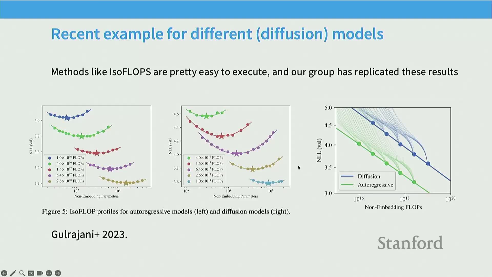
When applied to novel modeling paradigms (e.g., text diffusion models), the same empirical playbook (isoslop/isoflop analyses) often produces predictable scaling behavior with curves that mirror autoregressive results up to constant offsets.
-
Mechanism: training grids for alternative architectures and plotting minimum loss envelopes often reveals parallel power‑law behavior, indicating scaling phenomena are not idiosyncratic to one objective or decoder.
-
Rationale: cross‑model reproducibility supports using scaling‑law analysis as a general engineering tool when exploring new model families, subject to careful experimental control.
-
Implementation note: confirm offset magnitudes and that the productive regime exists for the new architecture before extrapolating to extreme scales.
Log-linear scaling across data, parameters, and compute provides a unifying empirical foundation for many practical model-design and resource-allocation decisions
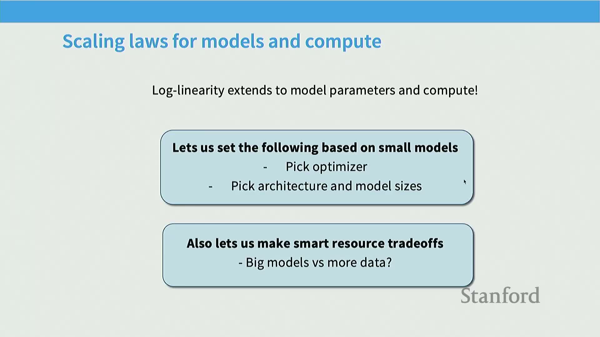
Power‑law (log‑log linear) relationships often hold across multiple axes — dataset size, parameter count, compute — enabling unified analyses for architecture selection, hyperparameter transfer, iso‑flop optimization, and batch/learning‑rate scheduling.
-
Mechanism: these empirical regularities permit dimensionality reduction of design choices into simple curves or surfaces that teams can fit on small‑to‑moderate experiments and extrapolate to production scales.
-
Practical impact: guidance on tokens‑per‑parameter ratios, when to prefer more data versus more parameters, and how to design scale‑stable parameterizations for optimizer transfer.
-
Caveats: validate scaling assumptions for downstream tasks, account for training‑schedule interactions, and quantify fit uncertainty.
-
Summary implication: when properly validated, scaling laws materially reduce the risk and cost of building large‑scale generative models by turning extensive empirical sweeps into concise, actionable extrapolations.
Enjoy Reading This Article?
Here are some more articles you might like to read next: