CS336 Lecture 10 - Inference
- Lecture introduction and scope of inference
- Inference importance and primary metrics (TTFT, latency, throughput)
- Training parallelism versus sequential nature of autoregressive inference
- Transformer notation and computational graph review
- Arithmetic intensity analysis for matrix multiplication and accelerator limits
- Implication of low arithmetic intensity (B=1) for generation
- KV caching to eliminate prefix recomputation during autoregressive generation
- Transformer MLP and attention IO/flop accounting and resulting intensities
- Prefill is compute-limited while generation is memory-limited
- Latency and throughput modeling with a concrete Llama 2 13B H100 example
- Scaling via replicated model instances and model sharding
- Group Query Attention (GQA) reduces KV cache size by sharing key/value heads
- Multi-Head Latent (MLA) projection for compact KV representations
- Cross-Layer Attention (CLA) shares KV projections across layers to reduce cache
- Local attention and hybrid architectures to cap KV growth
- Alternative architectures: state-space models, Hyena/Mamba and linear attention at scale
- Diffusion-based and parallel-generation approaches for faster sampling
- Quantization techniques for inference memory and bandwidth reduction
- Model pruning and structured sparsity with distillation to recover accuracy
- Speculative decoding using a cheap draft model to accelerate exact sampling
- Serving dynamics, batching heterogeneity, and memory allocation strategies (page attention)
Lecture introduction and scope of inference
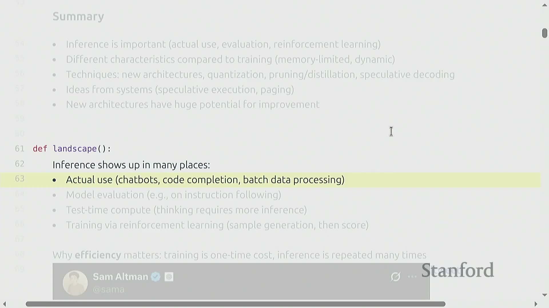
Inference denotes the process of generating model outputs from a fixed, pre-trained model given prompts and appears across multiple use cases including chat, code completion, batch processing, evaluation, and reinforcement-learning-based training.
Inference is distinct from training because it is executed repeatedly at runtime and therefore often dominates operational cost and the user experience for deployed systems.
This lecture positions inference as a broad topic that spans:
-
Workload characterization — understanding request shapes, sequence lengths, and batching patterns
-
System-level optimizations — kernels, memory layout, and scheduling
-
Architectural changes — model modifications that trade compute, memory, and accuracy for improved latency and throughput
Inference importance and primary metrics (TTFT, latency, throughput)
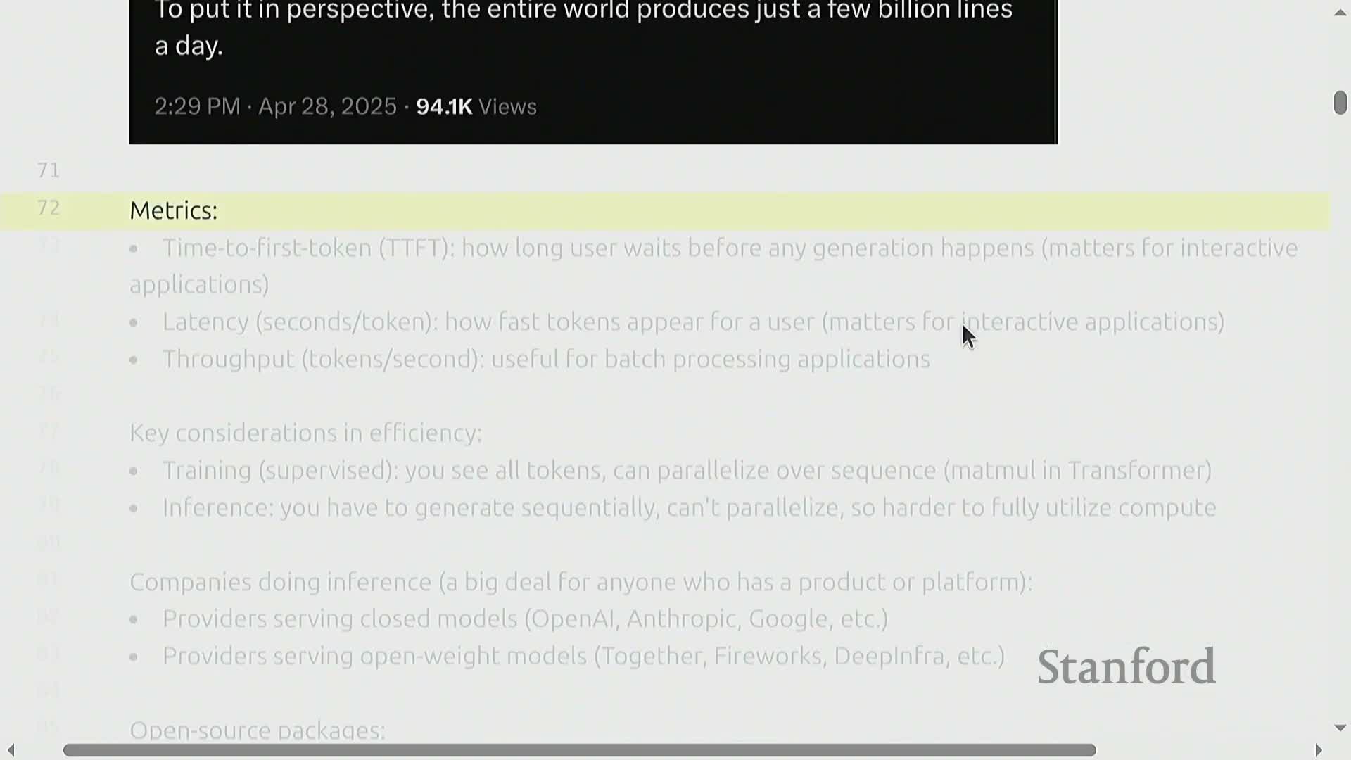
Practical evaluation of inference hinges on three primary metrics:
-
Time-to-first-token (TTFT) — the elapsed time until any token is produced; a key determinant of interactivity.
-
Latency — the per-request token arrival speed that affects perceived responsiveness for an individual request.
-
Throughput — the aggregate tokens produced per unit time, which matters for batch and high-volume workloads.
These metrics trade off with one another:
- Optimizing throughput (e.g., via large batching) can worsen per-request latency and TTFT.
- Minimizing TTFT typically reduces achievable throughput.
Quantifying and balancing these metrics guides architecture and system decisions for production deployments.
Training parallelism versus sequential nature of autoregressive inference
-
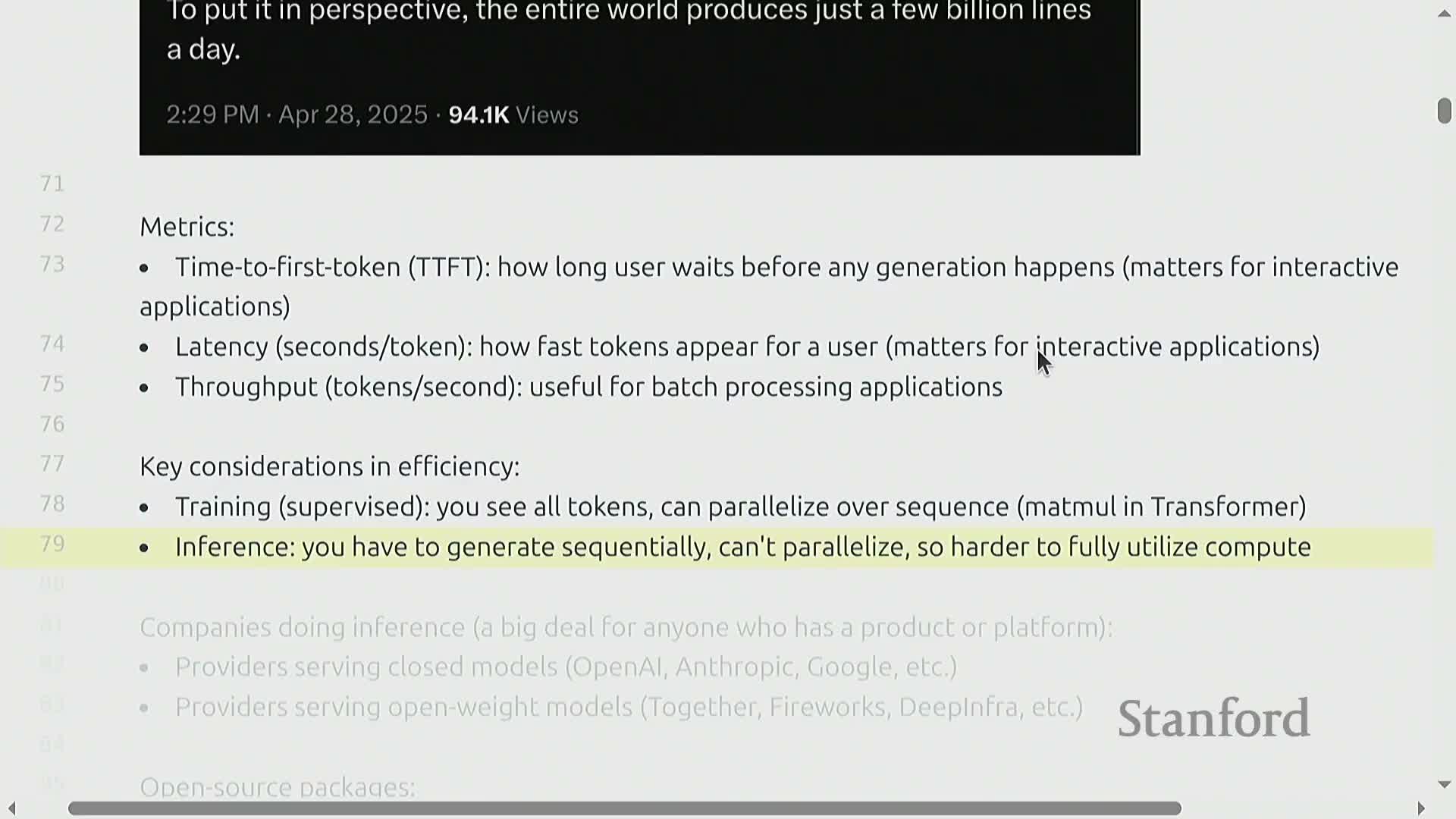
Training typically exploits full-sequence parallelism because all tokens are available at once, enabling efficient tensorized operations across sequence length.
-
Autoregressive inference, by contrast, requires sequential token generation: each output token conditions on prior outputs, preventing simple parallelization over the output sequence.
That sequential dependence creates two fundamental challenges:
-
Utilization problems — accelerators cannot be kept fully busy when generation is stepwise.
-
Memory pressure — per-step state (e.g., KV caches) must be stored and moved frequently.
As a result, inference is often more resource-constrained and operationally different from training.
Transformer notation and computational graph review
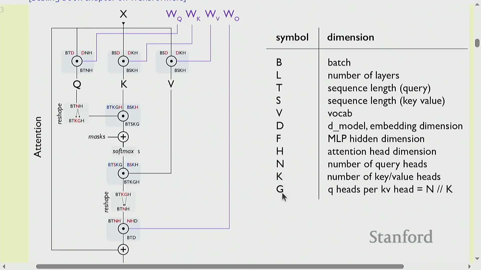
Transformer inference computation is organized by the key symbols:
-
B — batch size
-
L — number of layers
-
S — conditioning (prompt) sequence length
-
T — generated sequence length
-
D — model dimension
-
F — MLP hidden dimension
-
H — head dimension
-
N, K — query and key/value head counts respectively
Typical transformer computation alternates attention and MLP blocks, each expressed via large matrix multiplications and tensor contractions.
-
Attention introduces an O(S*T) term because queries interact with keys/values across conditioning and generated tokens.
-
MLPs contribute roughly O(BTD*F) floating-point operations per layer.
Expressing compute and memory in these symbols enables precise flop and byte-transfer accounting for later arithmetic intensity and performance analysis.
Arithmetic intensity analysis for matrix multiplication and accelerator limits
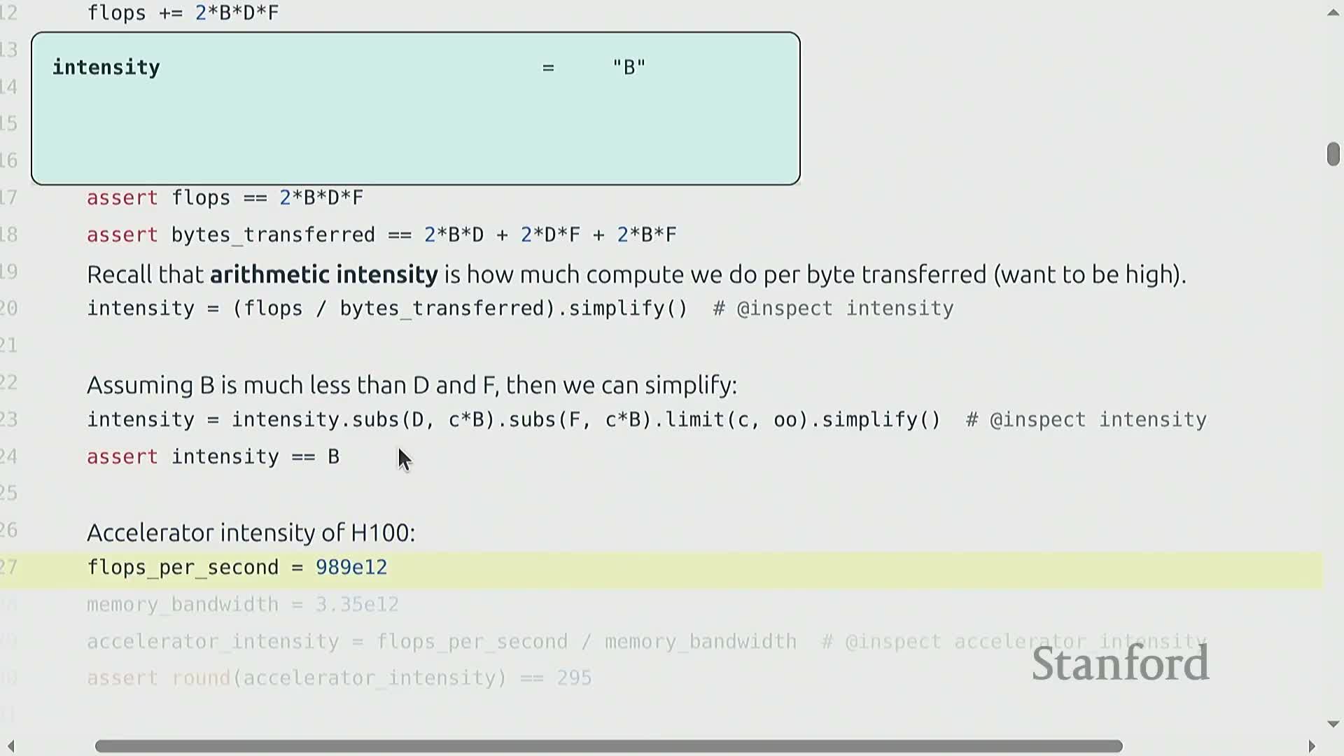
Arithmetic intensity is the ratio of floating-point operations to bytes transferred and determines whether a kernel is compute-bound or memory-bound on a given accelerator.
For a B×D times D×F matrix multiply:
- Flops scale as approximately 2·B·D·F.
- Bytes transferred include reads/writes of the input X, weights W, and the output, so the intensity simplifies to a quantity that is roughly proportional to the batch size B under common scalings.
Comparing this intensity to an accelerator’s peak flop-to-bandwidth ratio identifies thresholds (for example, an H100 requires B on the order of hundreds) below which the operation is memory-bound and cannot saturate compute.
Implication of low arithmetic intensity (B=1) for generation
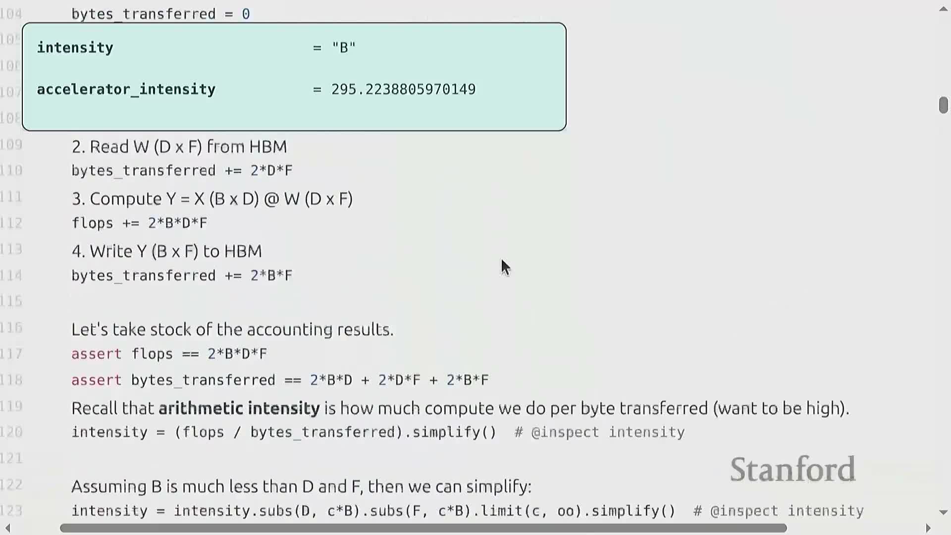
When B = 1 (matrix-vector products) or when sequence parallelism is absent, arithmetic intensity collapses toward one, implying severe memory-boundedness.
Consequences:
- Memory-bound kernels perform few flops per byte moved, so data transfers dominate runtime.
- Autoregressive generation often operates with small effective B and with T = 1 per generation step, making it inherently memory-limited and inefficient on modern accelerators unless mitigated.
KV caching to eliminate prefix recomputation during autoregressive generation
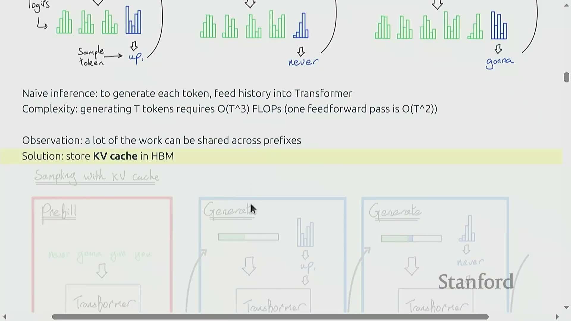
Autoregressive generation repeats much of the same prefix computation for each new token; KV caching avoids recomputing those prefix contributions by storing per-layer key and value projections in high-bandwidth device memory.
Two phases:
-
Prefill — compute and store the KV cache for the prompt in parallel across tokens.
-
Generation — append new KV vectors per generated token and reuse the cached values to avoid recomputing prefix contributions.
Proper KV caching reduces computational complexity per generated token in naive analysis from O(T^2) to O(T) and is essential for practical transformer inference.
Transformer MLP and attention IO/flop accounting and resulting intensities
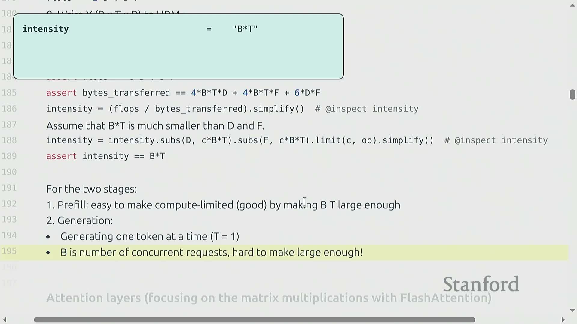
Per-layer accounting separates MLP and attention contributions:
-
MLP layers
- Perform large matrix multiplies with arithmetic intensity roughly proportional to B·T under typical parameter scalings.
- Batching and longer sequence lengths increase intensity, helping reach compute-bound regimes.
- Perform large matrix multiplies with arithmetic intensity roughly proportional to B·T under typical parameter scalings.
-
Attention layers
- Require Q×K matrix multiplies that scale as B·S·T·D and have memory reads proportional to the per-sequence KV cache size.
- A simplified attention intensity evaluates to approximately S·T / (S + T):
- During prefill this is O(S) (good — high intensity).
- During generation (T≈1) this collapses to O(1) (bad — low intensity).
- During prefill this is O(S) (good — high intensity).
- Require Q×K matrix multiplies that scale as B·S·T·D and have memory reads proportional to the per-sequence KV cache size.
Thus, attention inherently imposes a low, often-unimprovable arithmetic intensity during token-by-token generation because KV caches are sequence-specific and scale with batch.
Prefill is compute-limited while generation is memory-limited
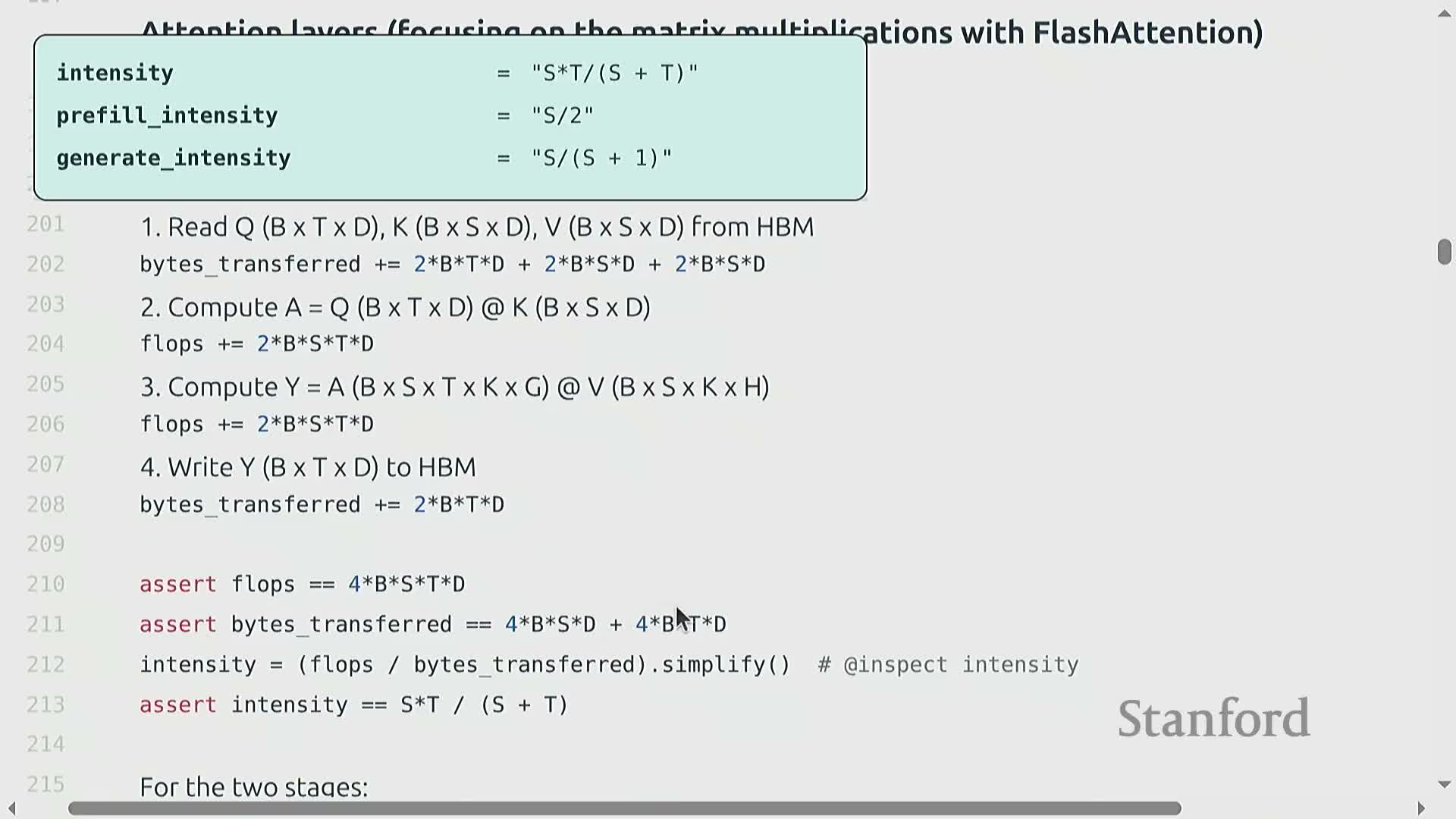
When encoding the prompt (prefill), computation can be parallelized across sequence and batches, so arithmetic intensity can be made large enough to be compute-bound, allowing near-saturated accelerators.
By contrast, the generation stage produces tokens sequentially (T≈1), which:
- Reduces effective arithmetic intensity.
- Renders inference memory-bound due to frequent KV cache transfers.
Consequently, optimization strategies differ:
-
Prefill benefits from heavyweight compute kernels and large batch/sequence parallelism.
-
Generation must minimize memory transfers and the KV footprint to improve latency and throughput.
Latency and throughput modeling with a concrete Llama 2 13B H100 example
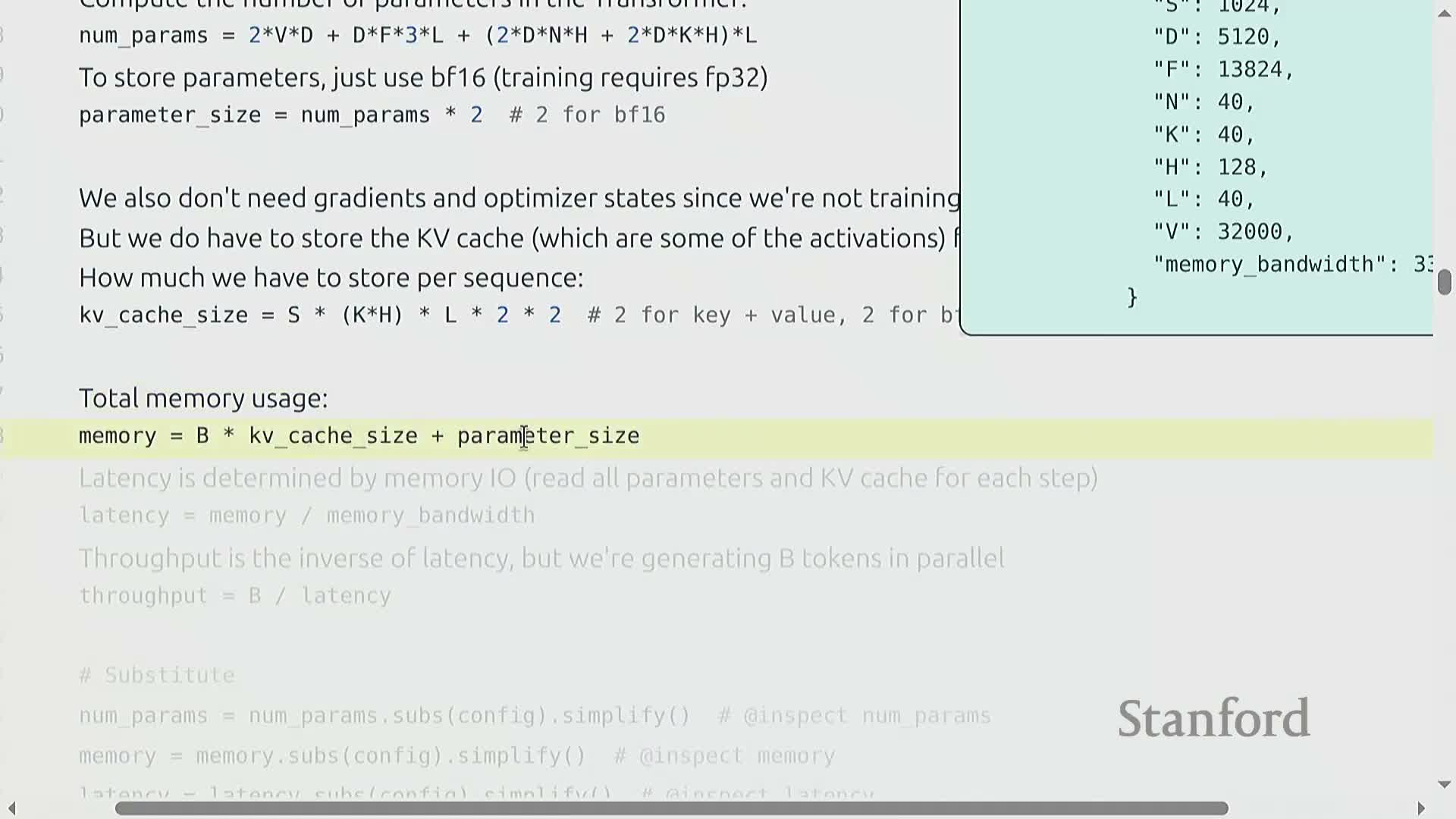
A stylized model that assumes perfect overlap of compute and communication provides tractable latency and throughput estimates by dividing required byte transfers by device memory bandwidth to estimate per-token latency and scaling throughput by batch size B.
Example instantiation (qualitative takeaways):
- For a Llama-2-like 13B model on an H100, single-request (B = 1) generation can yield millisecond-range per-token latencies and modest tokens/sec throughput.
- Increasing B raises throughput but also increases memory and per-request latency, exhibiting diminishing returns and hard caps set by on-device memory capacity.
This quantitative instantiation demonstrates the latency/throughput trade-offs and memory ceilings that govern practical inference.
Scaling via replicated model instances and model sharding
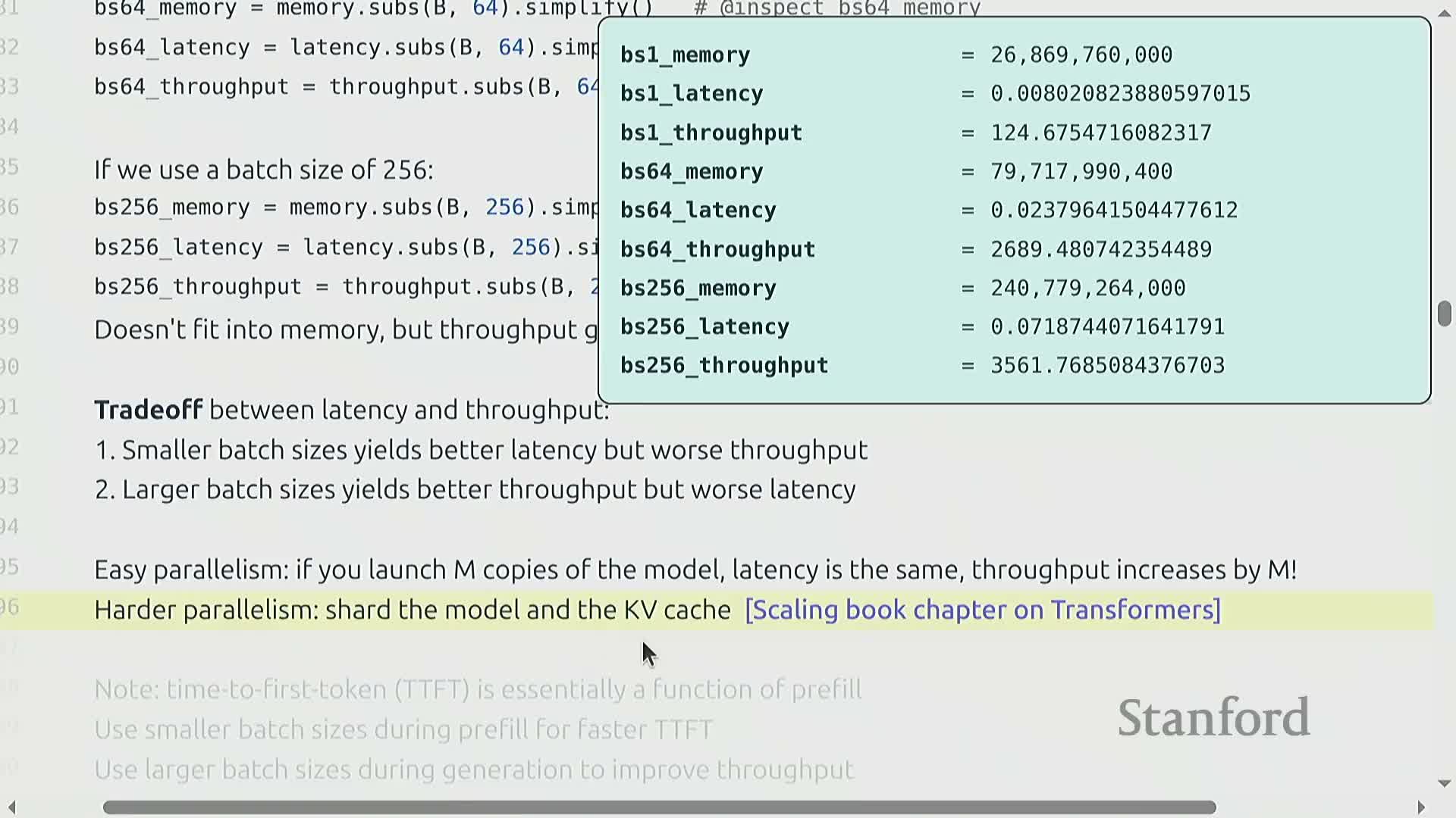
A simple parallelism strategy for serving is model replication:
- Run M independent copies of the model to increase overall throughput by M without inter-model communication.
- Replication preserves per-request latency but multiplies memory requirements.
When a single model replica cannot fit on-device, parameter and KV cache sharding across accelerators becomes necessary:
- Sharding introduces communication and coordination overheads.
- KV cache layout and sharding strategy materially affect memory transfers and performance.
Both replication and sharding are viable levers to tune throughput subject to memory and communication constraints.
Group Query Attention (GQA) reduces KV cache size by sharing key/value heads
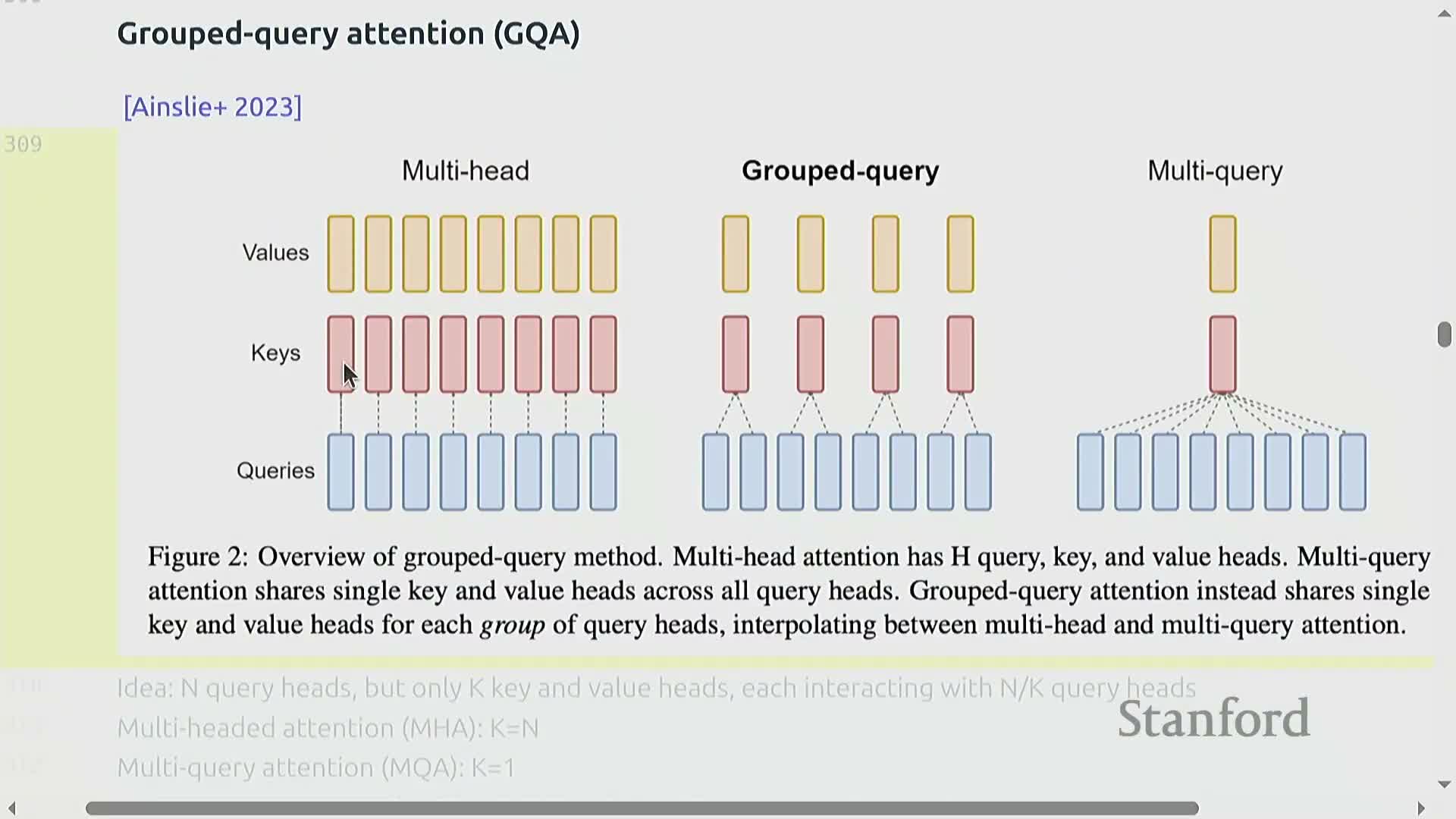
Group Query Attention (GQA) reduces KV cache memory by using fewer key/value (K/V) heads than query heads.
Key ideas and effects:
- Multiple query heads share the same K/V representations, shrinking per-token KV storage proportional to the reduction in K/V head count.
- This preserves query expressivity while reducing KV memory, enabling larger batch sizes and higher throughput on the same device memory budget.
- Empirical results show substantial latency and throughput gains with negligible accuracy loss up to moderate grouping ratios, making GQA an effective low-loss inference optimization.
Multi-Head Latent (MLA) projection for compact KV representations
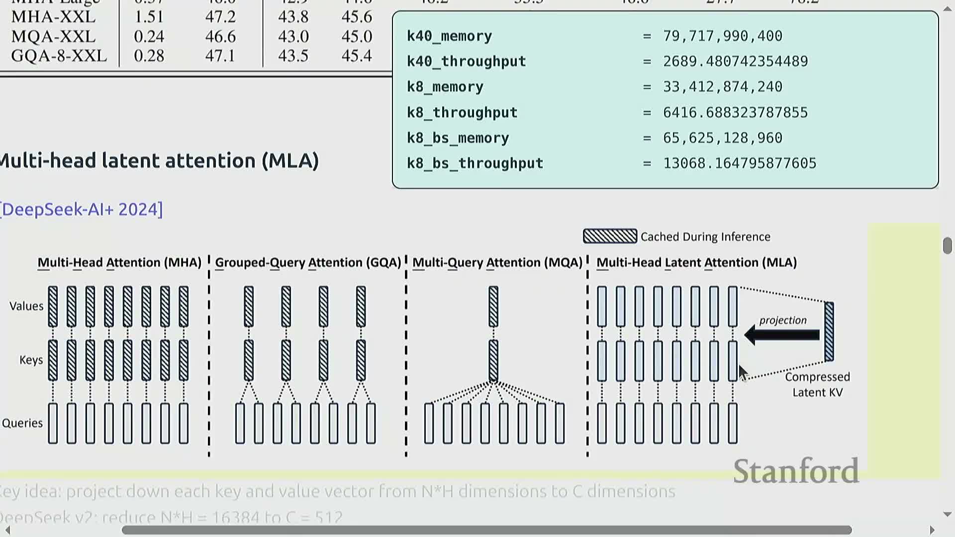
Multi-Head Latent (MLA) methods compress KV storage by projecting per-token KV vectors into a lower-dimensional latent space rather than reducing head count.
Characteristics:
- MLA dramatically shrinks the KV footprint (e.g., tens of thousands → a few hundred dimensions) while retaining useful representational capacity.
- Practical implementations must reconcile positional encodings (such as RoPE) with dimensionality reduction to preserve sequence information.
- When properly implemented, MLA delivers latency and throughput benefits comparable to head-count reduction techniques while maintaining accuracy with modest architectural adjustments.
Cross-Layer Attention (CLA) shares KV projections across layers to reduce cache
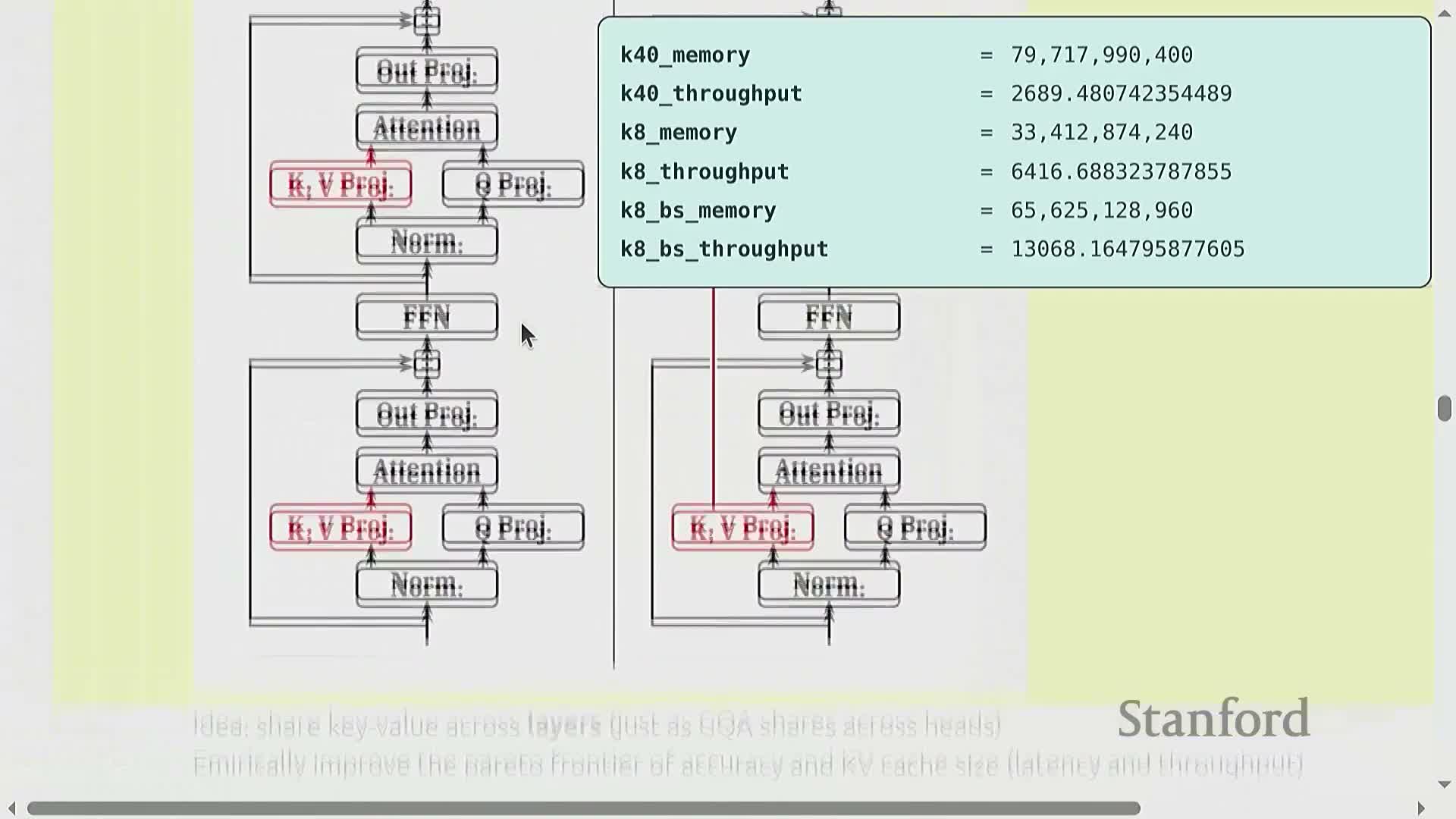
Cross-Layer Attention (CLA) collapses per-layer KV projections into shared projections that are reused across multiple consecutive layers, reducing KV cache storage across the stack.
Trade-offs and effects:
- By amortizing KV storage across layers, CLA lowers on-device memory pressure and can improve the latency/throughput frontier.
- It trades off some representational flexibility and can slightly affect perplexity.
- Empirical evidence indicates favorable trade-offs in many settings, especially when combined with other KV-reduction techniques.
Local attention and hybrid architectures to cap KV growth
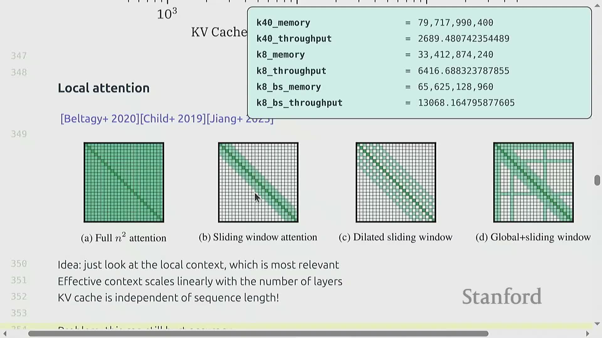
Local attention restricts attention to a fixed window of the past K tokens so KV cache size remains bounded and does not grow with sequence length, turning per-sequence KV cost into a constant rather than O(S).
To recover long-range modeling capacity, hybrid designs:
- Interleave local attention layers with occasional global attention layers.
- Combine local patterns with KV-sharing techniques.
Such local-and-global hybridization is a pragmatic balance between memory-efficient inference and long-range dependency modeling and is used in production systems to preserve much of transformer expressivity while greatly reducing KV memory and quadratic cost.
Alternative architectures: state-space models, Hyena/Mamba and linear attention at scale
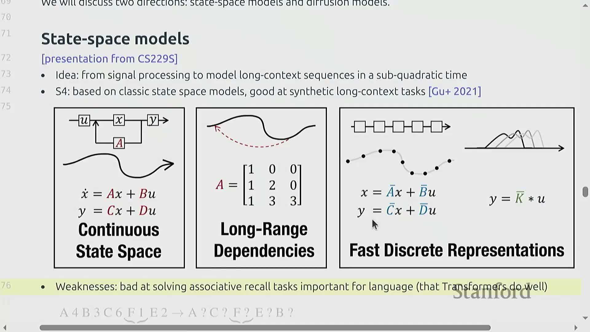
State-space models (SSMs) and recent variants such as Hyena and Mamba reinterpret sequence modeling through linear dynamical systems or convolutional kernels to avoid full O(S^2) attention and to enable RNN-like or convolutional implementations.
Key points:
- These architectures were motivated by long-context efficiency and have been adapted with transformer components or occasional full-attention layers to handle associative recall tasks needed for language.
- Linear-attention variants and hybrid stacks have been scaled to very large parameter counts (hundreds of billions), showing that much of the transformer can be replaced with lower-KV, linear-or-local components while preserving competitive performance.
Diffusion-based and parallel-generation approaches for faster sampling
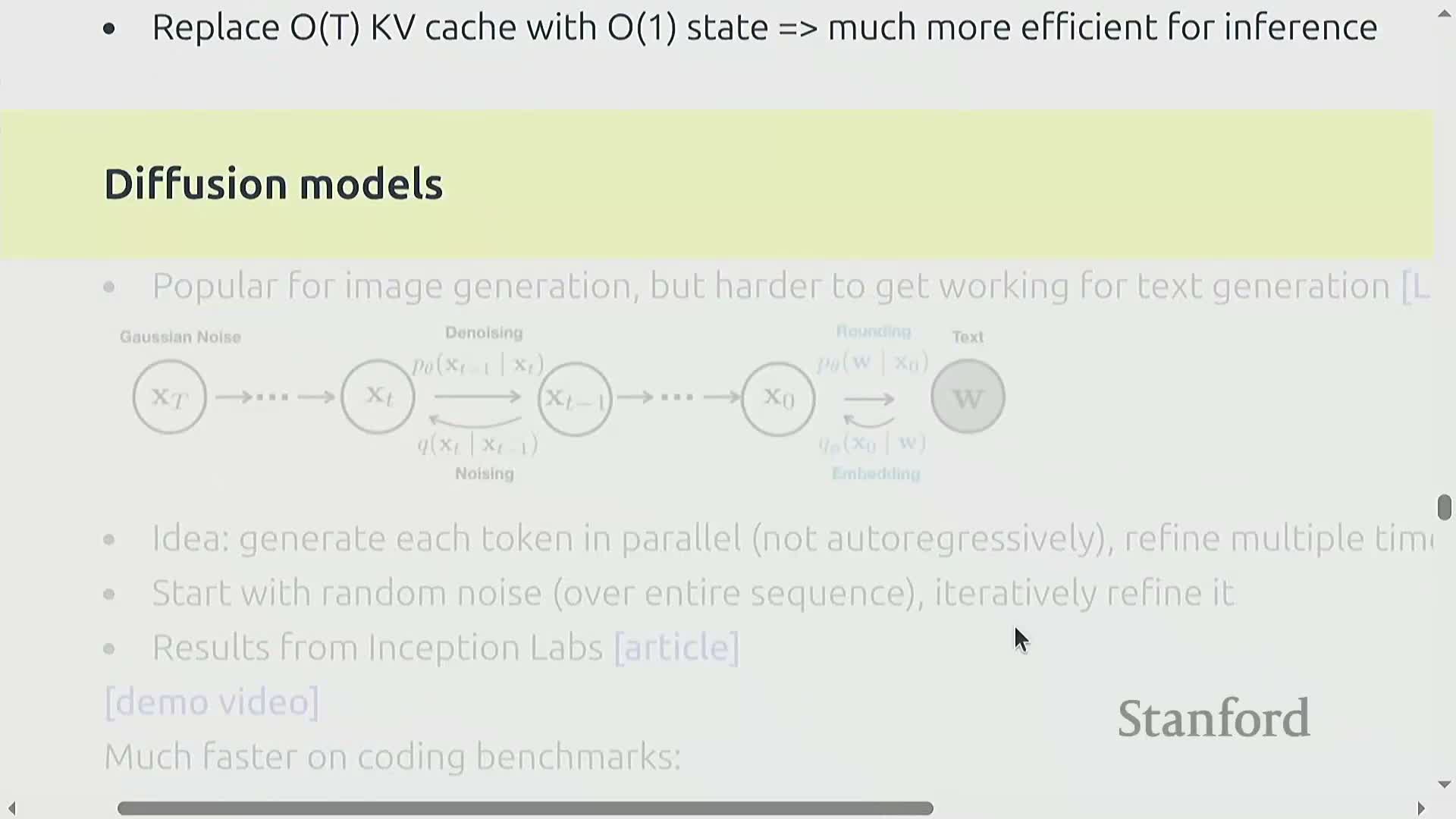
Diffusion-style text generation iteratively refines full-sequence drafts in parallel rather than generating tokens autoregressively, enabling strong parallelism and very high tokens-per-second throughput.
How it works and trade-offs:
- The approach produces initially noisy outputs that are progressively denoised or refined over multiple iterations; each iteration operates on the whole sequence and can be executed in parallel across devices, eliminating per-token sequential KV transfers.
- Early results, particularly on coding tasks, show dramatic speed advantages versus autoregressive transformers.
- Achieving parity in general language accuracy remains an active research challenge.
Quantization techniques for inference memory and bandwidth reduction
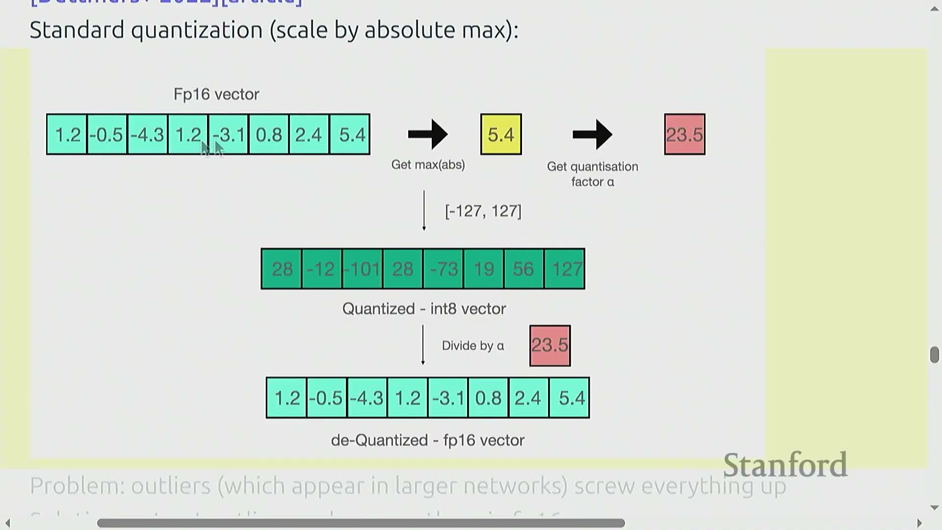
Quantization reduces numeric precision of weights and activations (e.g., BF16 → FP8/INT8/INT4) to lower memory footprint and bandwidth requirements, directly reducing the dominant memory transfer cost of generation.
Practical strategies include:
-
Post-training quantization and dynamic schemes that isolate and preserve outlier parameters or activations in higher precision (for example, keeping a small set of large-magnitude columns in FP16 while quantizing the rest to INT8).
-
Activation-aware and mixed-precision pipelines that enable aggressive compression with modest accuracy loss.
When implemented with hardware-aware kernels, quantization yields substantial runtime and memory benefits.
Model pruning and structured sparsity with distillation to recover accuracy
Structured pruning removes entire layers, attention heads, or hidden dimensions judged unimportant by calibration, producing smaller, faster variants of a trained model.
To mitigate accuracy degradation, the pruned architecture is typically:
-
Reinitialized, and then
-
Distilled from the full model to transfer behavior and calibrate the reduced parameterization.
This combination of selection and distillation has enabled meaningful parameter reductions (for example, from 15B → 8B) with small accuracy losses on common benchmarks, offering a practical path for cost-effective inference.
Speculative decoding using a cheap draft model to accelerate exact sampling
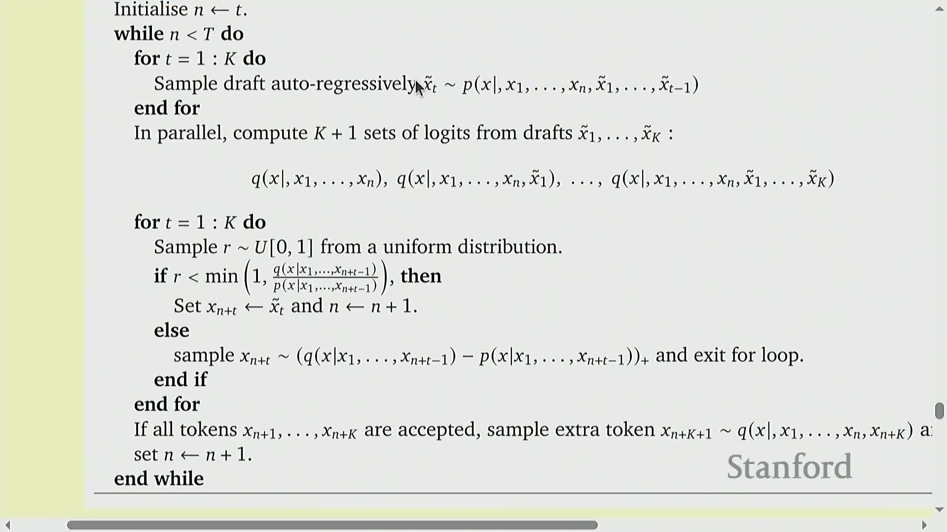
Speculative decoding uses a small, fast draft model P to generate multiple look-ahead tokens and then verifies those tokens under the target model Q via scoring (a prefill-like parallel evaluation) to accept or reject proposals.
Procedure and guarantees:
- Accepted tokens are returned immediately; rejected proposals are corrected by sampling from Q.
- The overall procedure is constructed so that accepted outputs are exact samples from Q, preserving model correctness.
- Because verification uses parallel prefill-like operations and drafting is cheap, speculative decoding can yield significant wall-clock speedups while producing mathematically exact samples from the expensive target distribution.
Serving dynamics, batching heterogeneity, and memory allocation strategies (page attention)
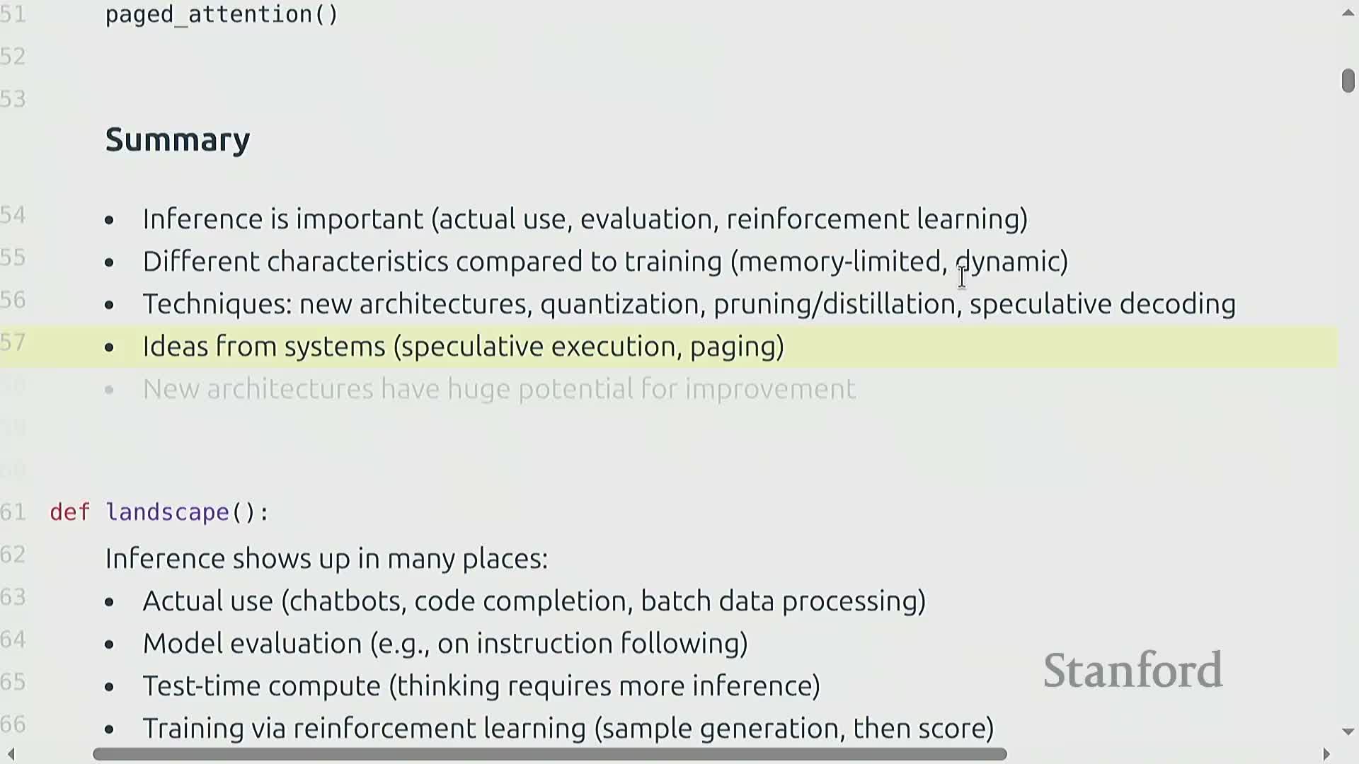
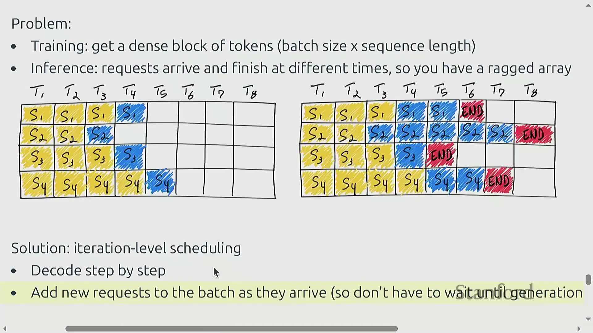
Real-world serving traffic is heterogeneous with varying arrival times, request lengths, and shared prefixes, creating fragmentation and scheduling challenges that differ from dense training workloads.
Systems strategies to address these issues include:
-
Selective batching — flatten independent MLP computations while handling attention per-request.
-
Copy-on-write prefix sharing — avoid duplicating KV blocks for requests that share prefixes.
-
Page-based KV allocation — break the KV cache into contiguous blocks for flexible reuse and compaction.
Applying operating-system-inspired memory management and dynamic scheduling reduces fragmentation, improves memory utilization, and increases effective throughput under live traffic loads.
Enjoy Reading This Article?
Here are some more articles you might like to read next: