CS336 Lecture 17 - Alignment - RL - Part 2
- Course orientation and lecture goals
- Reinforcement learning formulation for language models: states, actions, rewards, and dynamics
- Policy and objective in outcome-reward LM reinforcement learning
- Policy gradient derivation: gradient of expected reward via log-derivative trick
- Naive policy gradient as reward-weighted supervised fine-tuning and implications of binary rewards
- Dataset non-stationarity and contrast with continuous reward RLHF
- Baselines for variance reduction in policy gradient
- Toy two-state example illustrating variance pitfalls and baseline benefits
- Optimal baseline expression and practical heuristic choice
- Advantage function and unified delta notation for algorithms
- GRPO lineage and group-structured variance reduction in LM settings
- Toy sorting task and reward design alternatives
- Simplified model architecture and sampling strategy for the sorting task
- Computing deltas: centering, normalization, and optional max-only selection
- Log-probability extraction and naive policy-gradient loss computation
- Freezing reference quantities (no-grad) and importance-ratio pitfalls
- Credit assignment and discounting considerations for outcome rewards
- GRPO clipped objective and KL regularization
- Algorithm components, inner/outer loop structure, and computational workflow
- Why a separate KL reference vs. old policy and initialization considerations
- Empirical sorting-task experiments and learning curve interpretation
- Conclusions: promise of RL for LMs and scaling challenges
mindmap
Policy-gradient RL for LMs outcome rewards
LM formulation
state = prompt + tokens
action = next token / whole response
transition = append
reward = outcome sparse, delayed
Gradient & deltas
score-function estimator
advantage = return − Vs
delta = reward/centered/normalized
Variance reduction
state-dependent baselines
centering & normalization
no-grad cached pi_old
GRPO & grouped updates
multiple responses per prompt
per-prompt baselines group mean
clipping + KL reference
Reward design
binary vs shaped rewards
partial credit position/adjacency
max-only vs smooth shaping
Implementation & workflow
outer rollouts, inner optimization
cache logits, freeze references
tradeoff: inference cost vs samples
Challenges & scaling
sparse rewards & credit assignment
high Monte Carlo variance
engineering: multi-model orchestration
Course orientation and lecture goals
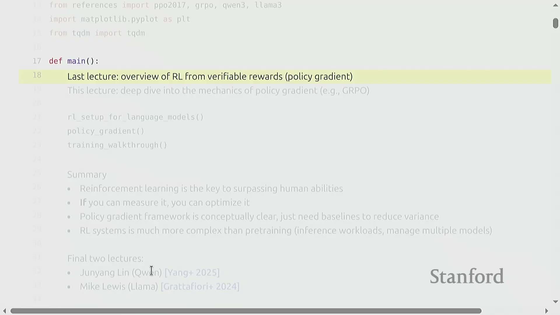
This session is positioned at the end of the quarter and will deep-dive into policy gradient methods for reinforcement learning (RL) applied to language models (LMs).
- Goals:
- Expand on prior coverage of RL with verifiable rewards rather than introduce fundamentally new theory.
- Provide mathematical detail and code-oriented examples that connect theory to practice.
- Focus on algorithm mechanics (e.g., policy gradients, GRPO) and on practical implementation concerns.
- Expand on prior coverage of RL with verifiable rewards rather than introduce fundamentally new theory.
- Framing:
- Treats the lecture as a continuation and an application-focused elaboration of earlier material.
- Treats the lecture as a continuation and an application-focused elaboration of earlier material.
Reinforcement learning formulation for language models: states, actions, rewards, and dynamics
-
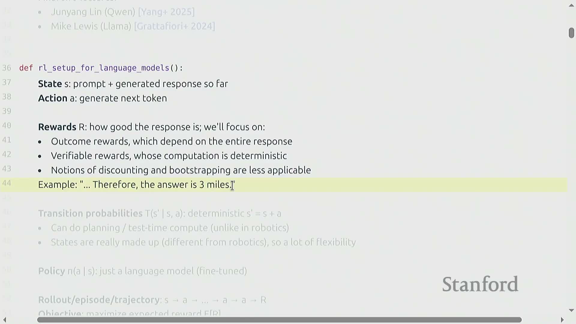
State (LM setting): the prompt concatenated with the tokens generated so far.
-
Action: generating the next token.
- Reward characteristics:
-
Outcome-based and deterministic: rewards depend on the entire generated response (verifiable).
- This makes signals sparse and delayed, but conceptually simpler than interactive environments.
-
Outcome-based and deterministic: rewards depend on the entire generated response (verifiable).
- Transition dynamics:
- Trivial string concatenation: state’ = state + action.
- This simplicity enables planning or test-time computation that physical robotics typically cannot use.
- Trivial string concatenation: state’ = state + action.
- State representation challenges:
- The LM synthesizes arbitrary internal tokens, so states are ungrounded text and can include internal scratchpad behavior.
- Main challenge: ensure those token sequences produce verifiable, correct outcomes rather than merely reaching reachable but meaningless states.
- The LM synthesizes arbitrary internal tokens, so states are ungrounded text and can include internal scratchpad behavior.
Policy and objective in outcome-reward LM reinforcement learning
-
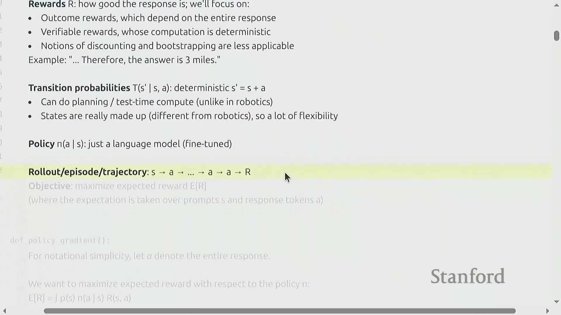
Policy: an LM conditioned on the current token sequence (prompt + generated tokens).
-
Training objective: maximize expected reward over the distribution of prompts and the policy’s token outputs.
- Outcome-reward simplification:
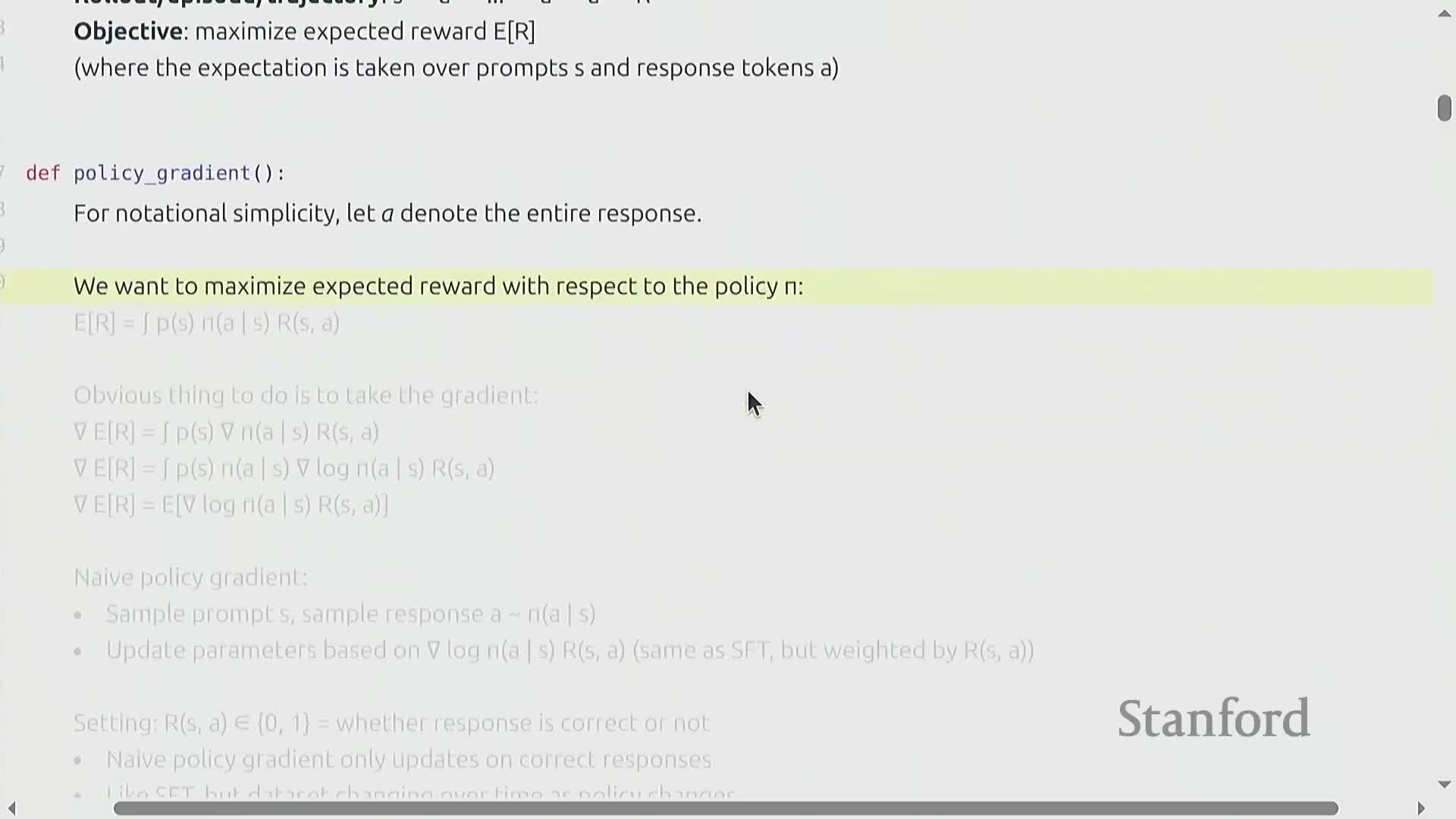
- When rewards are outcome-based, treat the entire response as a single action a with a single reward R.
- This yields a simpler expected-reward expression and implementation.
- When rewards are outcome-based, treat the entire response as a single action a with a single reward R.
- Practical setup:
- Policies often initialize from pretrained LMs and are then fine-tuned via policy optimization.
-
Rollouts produce trajectories that yield a scalar reward at episode end.
- The objective integrates over environment-provided prompts and the stochastic policy’s responses to compute the expected return, which is the target for gradient-based optimization.
- Policies often initialize from pretrained LMs and are then fine-tuned via policy optimization.
Policy gradient derivation: gradient of expected reward via log-derivative trick
- Derivation sketch:
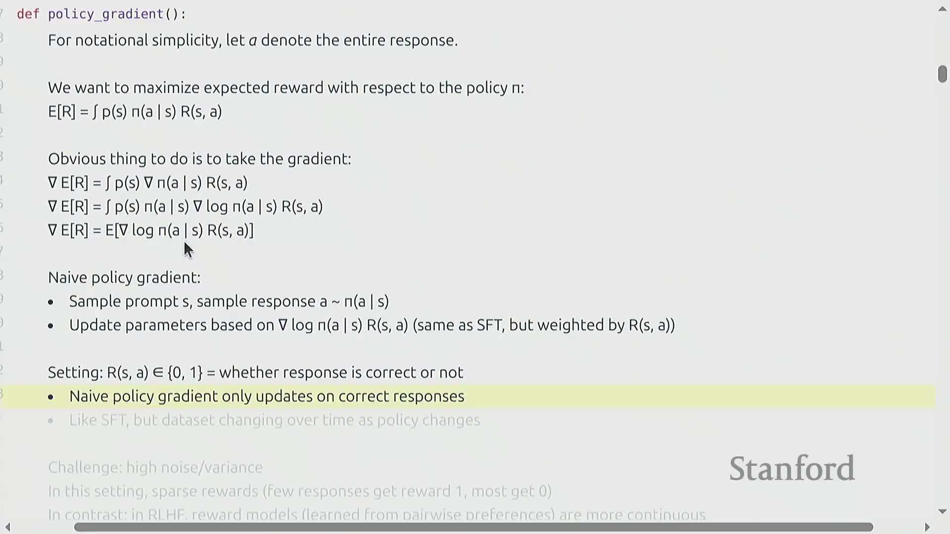
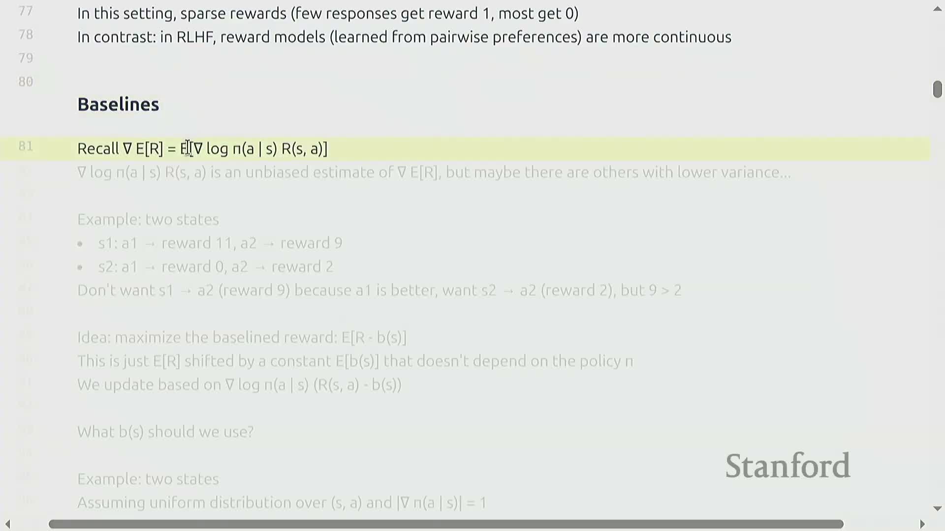
- Differentiate expected reward w.r.t. policy parameters and apply the log-derivative (score function) identity to move the gradient inside the expectation.
-
Result: an expectation of **∇ log π(a s)** weighted by the return (reward).
- Differentiate expected reward w.r.t. policy parameters and apply the log-derivative (score function) identity to move the gradient inside the expectation.
- Properties:
- This gives an unbiased Monte Carlo estimator when sampling prompts and actions.
- In the outcome-reward setting, treating the entire response as a single action further simplifies notation and implementation.
- This score-function estimator is the basis for sampling-based updates that seek to increase expected reward.
- This gives an unbiased Monte Carlo estimator when sampling prompts and actions.
Naive policy gradient as reward-weighted supervised fine-tuning and implications of binary rewards
-
Naive policy gradient update:
- Sample prompts and model responses, then apply gradient steps proportional to the sampled reward.
- Analogy: similar to supervised fine-tuning (SFT), but responses are weighted by reward rather than matched to fixed human targets.
- Sample prompts and model responses, then apply gradient steps proportional to the sampled reward.
- Special cases and failure modes:
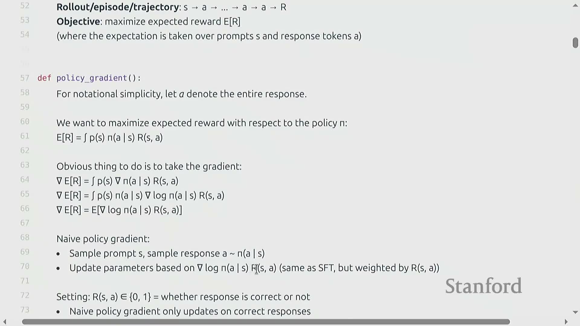
- With binary rewards (0/1), updates occur only for rewarded responses: effectively SFT on the subset of model outputs deemed correct.
- In sparse-reward regimes, if the policy rarely produces positive responses, gradients are near zero and learning can stall.
- Conclusion: naive sampling without variance reduction or reward shaping can leave the model stuck when initial performance is poor.
- With binary rewards (0/1), updates occur only for rewarded responses: effectively SFT on the subset of model outputs deemed correct.
Dataset non-stationarity and contrast with continuous reward RLHF
- Non-stationarity:
- Policy optimization changes the policy that generates training examples, so the empirical dataset evolves across iterations.
- This can be beneficial if the policy discovers easy positives and generalizes to harder prompts, but it complicates analysis and monitoring because the data distribution shifts.
- Policy optimization changes the policy that generates training examples, so the empirical dataset evolves across iterations.
- Reward-model contrast:
-
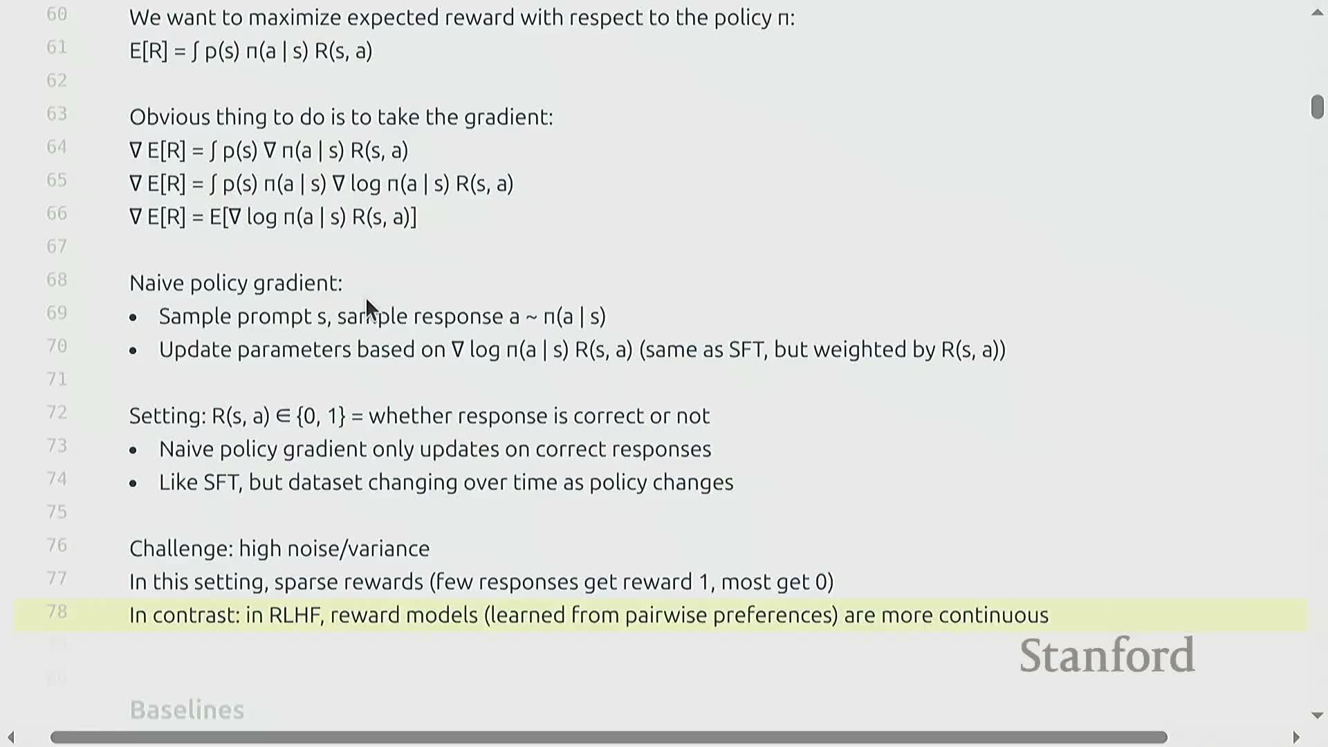
RL with human feedback typically uses a learned, continuous reward model, which provides graded values and reduces sparsity relative to binary verifiable rewards.
- The choice between verifiable outcome rewards and learned reward models affects algorithm design, hyperparameter choices, and intuitions about training dynamics.
-
RL with human feedback typically uses a learned, continuous reward model, which provides graded values and reduces sparsity relative to binary verifiable rewards.
Baselines for variance reduction in policy gradient
-
Baseline b(s):
- Any function of state (but not of action) that is subtracted from returns in the policy gradient estimator to reduce variance without biasing the gradient.
- Any function of state (but not of action) that is subtracted from returns in the policy gradient estimator to reduce variance without biasing the gradient.
- Why it’s unbiased:
- Subtracting b(s) leaves the expected gradient unchanged because the baseline term factors out of the expectation over actions for a given state and contributes zero in expectation.
- Subtracting b(s) leaves the expected gradient unchanged because the baseline term factors out of the expectation over actions for a given state and contributes zero in expectation.
- Practical notes:
- Baselines are fundamental to stabilize and accelerate convergence by centering the reward signal.
- Valid baselines include fixed constants or learned value estimators, provided they do not depend on the action.
- The design of b(s) substantially affects gradient variance and empirical learning speed.
- Baselines are fundamental to stabilize and accelerate convergence by centering the reward signal.
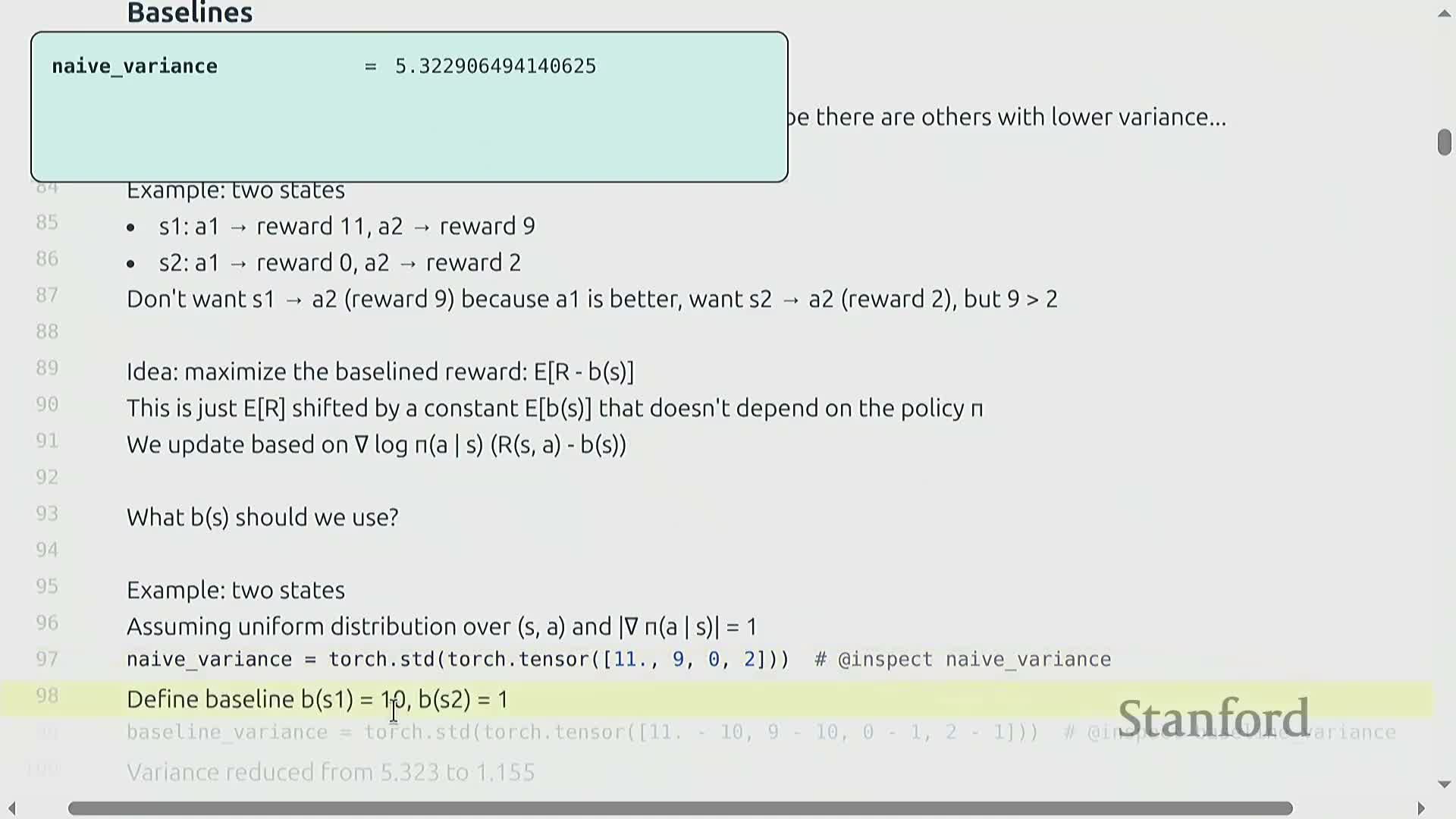
Toy two-state example illustrating variance pitfalls and baseline benefits
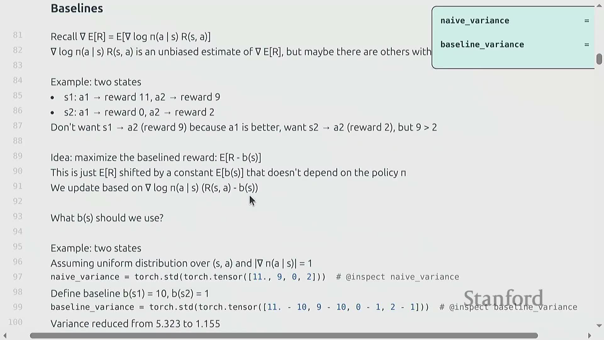
- Two-state toy example (intended insight):
- Two prompts (states) with different per-action rewards show how naive updates can favor misleadingly high absolute rewards in certain states and produce suboptimal policies.
- If the policy randomly selects an action that yields high reward in an easy state, repeated updates can amplify that action and eliminate the true global optimum—an instance of high-variance, myopic updates.
- Two prompts (states) with different per-action rewards show how naive updates can favor misleadingly high absolute rewards in certain states and produce suboptimal policies.
- Remedy:
- Introduce a state-dependent baseline (e.g., subtract per-state expected reward) to center rewards, dramatically reducing variance and preventing harmful relative gradients.
- The example quantifies how appropriate baselines can shrink variance by multiple factors and improve convergence behavior.
- Introduce a state-dependent baseline (e.g., subtract per-state expected reward) to center rewards, dramatically reducing variance and preventing harmful relative gradients.
Optimal baseline expression and practical heuristic choice
- Optimal baseline properties:
- For scalar-parameter models, the variance-optimal baseline has a closed-form involving expectations of squared score-function terms weighted by returns.
- In higher dimensions, the optimal solution requires covariance matrices and becomes impractical to compute exactly.
- For scalar-parameter models, the variance-optimal baseline has a closed-form involving expectations of squared score-function terms weighted by returns.
- Practical heuristic:
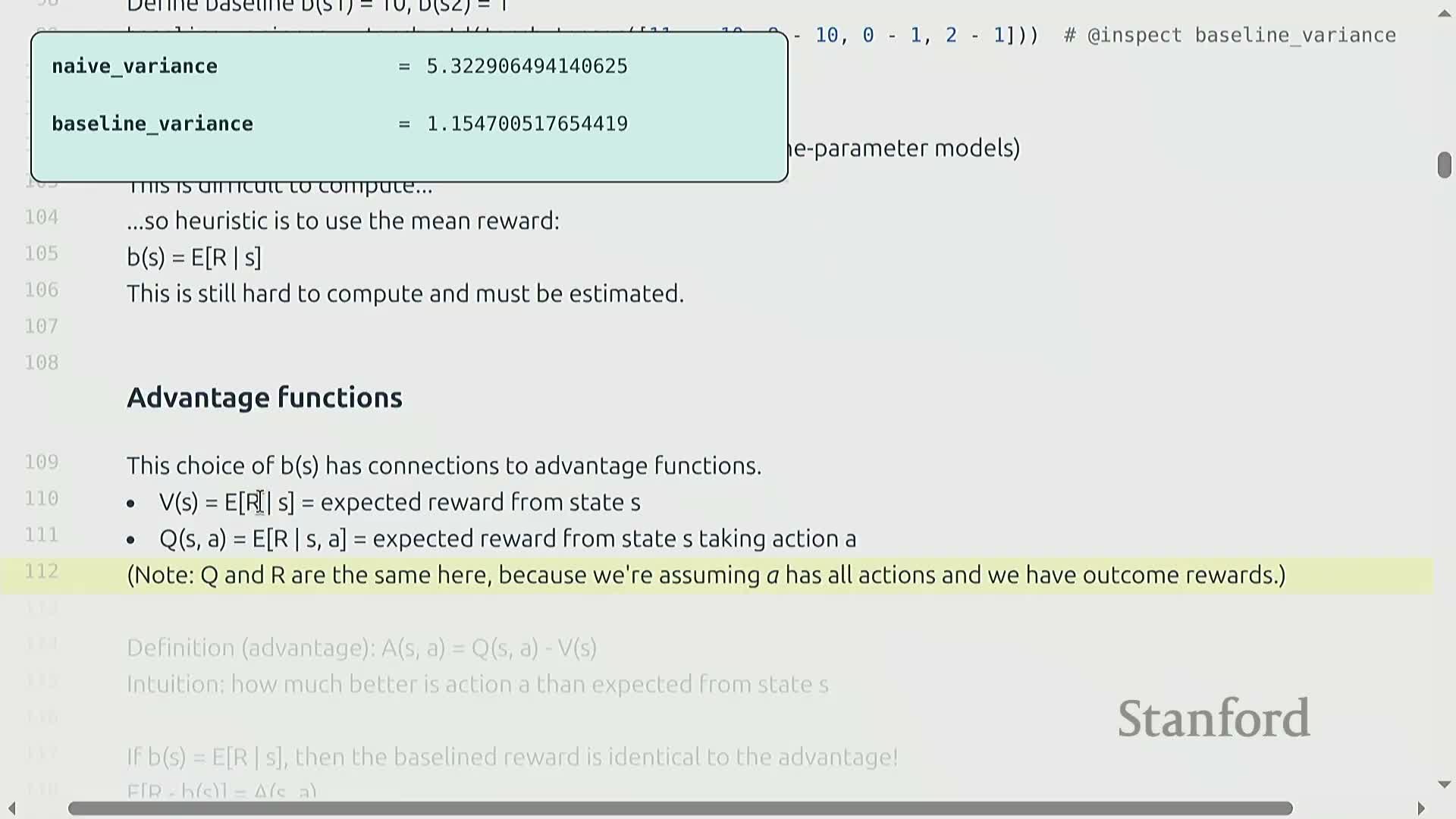
- Use the estimated expected reward given state (value estimate) as the baseline—this approximates the advantage function and typically yields substantial variance reduction.
- Value estimates are tractable to obtain via sampling or simple learned value functions, so implementations favor these computable approximations balancing cost and variance reduction.
- Use the estimated expected reward given state (value estimate) as the baseline—this approximates the advantage function and typically yields substantial variance reduction.
Advantage function and unified delta notation for algorithms
-
Advantage function A(s,a):
- Defined as Q(s,a) − V(s): how much better action a is relative to average behavior at state s.
- Provides a principled baseline choice when available.
- Defined as Q(s,a) − V(s): how much better action a is relative to average behavior at state s.
- Outcome-reward simplification:
- In the outcome-reward LM setting, Q and the return R coincide when treating the entire response as the return, so A = return − expected return given state.
- In the outcome-reward LM setting, Q and the return R coincide when treating the entire response as the return, so A = return − expected return given state.
- Implementation abstraction:
- Many algorithms adopt a unified scalar delta to represent whatever multiplier (reward, centered reward, normalized advantage, etc.) is used with the log-probability gradient.
- Variants differ primarily in how delta is computed, clarifying that modern policy-gradient techniques scale the score-function gradient by a carefully chosen delta to control variance and bias.
- Many algorithms adopt a unified scalar delta to represent whatever multiplier (reward, centered reward, normalized advantage, etc.) is used with the log-probability gradient.
GRPO lineage and group-structured variance reduction in LM settings
- Lineage and structure exploitation:
-
GRPO and related algorithms evolved from the PPO/DPO lineage but exploit structure specific to language modeling.
- Key LM structure: you can sample multiple responses per prompt, forming natural groups for per-prompt baselines (group means).
-
GRPO and related algorithms evolved from the PPO/DPO lineage but exploit structure specific to language modeling.
- Benefits of grouped sampling:
- Compute an empirical baseline across responses from the same prompt, which reduces variance without requiring a global learned value function.
- When rollouts are naturally grouped (many responses per prompt), GRPO-style relative updates are practical and effective.
- In environments without grouping, alternative value-estimation methods are required.
- Compute an empirical baseline across responses from the same prompt, which reduces variance without requiring a global learned value function.
- Algorithmic consequences:
- Group structure motivates clipping and normalization strategies that compare responses relative to their prompt-specific cohort.
- Group structure motivates clipping and normalization strategies that compare responses relative to their prompt-specific cohort.
Toy sorting task and reward design alternatives
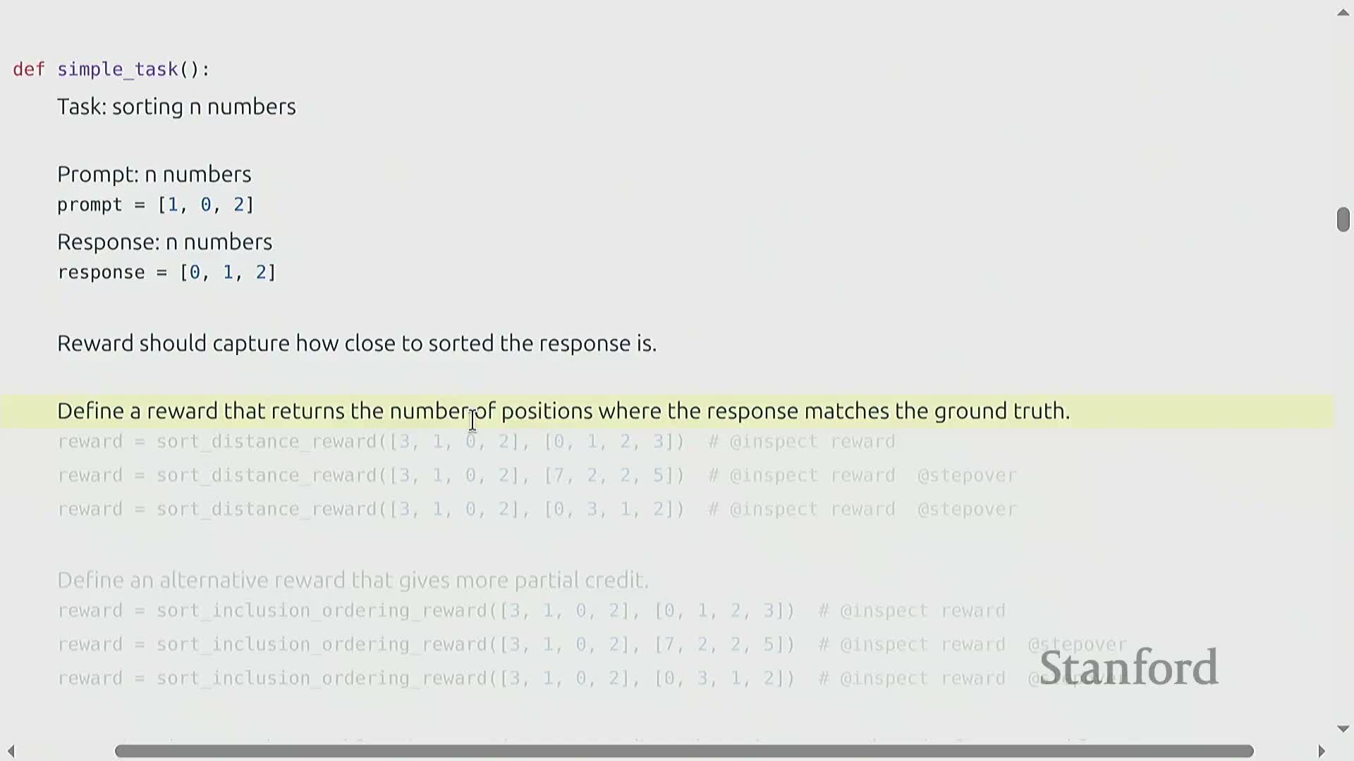
- Toy environment: sorting n numbers.
- Prompt: a sequence of numbers.
- Desired response: the sorted sequence.
- Reward must quantify closeness to ground truth.
- Prompt: a sequence of numbers.
- Possible reward formulations:
-
Binary correct/incorrect: severe sparsity.
-
Position-match counts: partial credit by summing positions that match the sorted result.
-
Inclusion-plus-adjacency: points for presence of prompt tokens and for correctly sorted adjacent pairs—richer shaping signals.
-
Binary correct/incorrect: severe sparsity.
- Reward-engineering trade-offs:
-
Too sparse: prevents learning.
-
Too permissive: can be exploited or mislead optimization.
- Designing a reward that balances informativeness and robustness is a critical practical decision.
-
Too sparse: prevents learning.
Simplified model architecture and sampling strategy for the sorting task
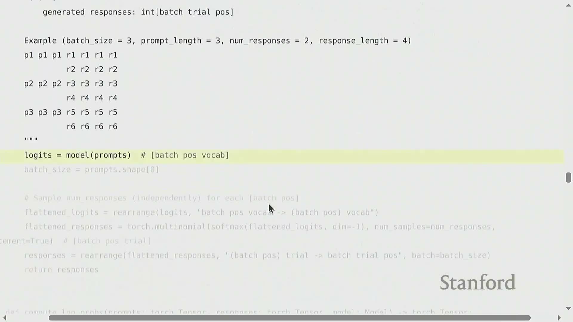
- Minimal parametric model for on-laptop experiments:
- Fixed, equal prompt and response lengths to simplify indexing.
-
Positional information captured via per-position parameter matrices.
-
Encoding collapses position embeddings into a prompt summary.
-
Decoding produces logits per response position independently (non-autoregressive) to simplify implementation.
- Fixed, equal prompt and response lengths to simplify indexing.
- Forward pass:
- Map batch-by-position inputs through embeddings and per-position linear transforms to produce logits over the vocabulary for each output position.
- Use logits to sample multiple response trials per prompt.
- Map batch-by-position inputs through embeddings and per-position linear transforms to produce logits over the vocabulary for each output position.
- Rationale:
- Trades realism for tractability but preserves core elements needed to illustrate policy-gradient training, grouped sampling, and reward-driven updates.
- Trades realism for tractability but preserves core elements needed to illustrate policy-gradient training, grouped sampling, and reward-driven updates.
Computing deltas: centering, normalization, and optional max-only selection
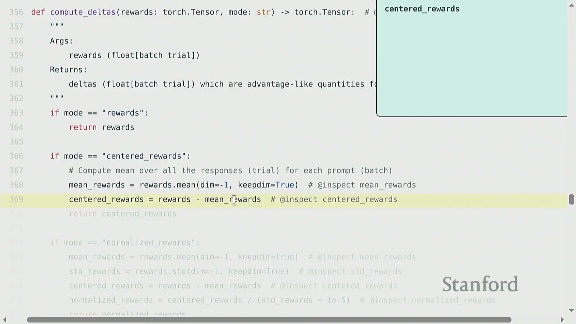
- compute_deltas: converts raw rewards into scalar multipliers for gradient updates. Common choices include:
-
Raw rewards (no transformation).
-
Centering by subtracting per-prompt means.
-
Normalization by dividing by standard deviation (with epsilon for numerical stability).
-
Max-only: zero out any response that is not the batch maximum.
-
Raw rewards (no transformation).
- Practical effects:
-
Centering turns sparse 0/1 rewards into both positive and negative signals, so incorrect responses produce negative updates and correct ones positive—helps learning when positives are rare.
-
Normalization yields scale invariance to multiplicative reward changes.
-
Max-only selection enforces an all-or-nothing strategy to avoid rewarding trivial partial-credit solutions.
-
Centering turns sparse 0/1 rewards into both positive and negative signals, so incorrect responses produce negative updates and correct ones positive—helps learning when positives are rare.
- Takeaway:
- The chosen delta transformation profoundly affects update direction, stability, and sensitivity to reward scaling.
- The chosen delta transformation profoundly affects update direction, stability, and sensitivity to reward scaling.
Log-probability extraction and naive policy-gradient loss computation
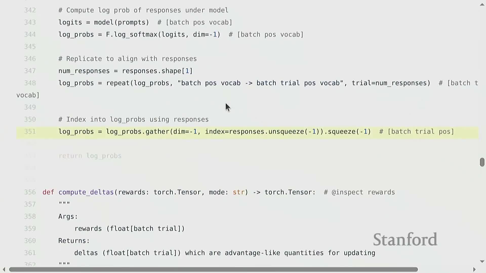
- Computing log-probabilities and loss:
- After sampling and scoring responses, compute the log-probability of each sampled token sequence by indexing model logits at the chosen token indices and summing or averaging across positions.
- After sampling and scoring responses, compute the log-probability of each sampled token sequence by indexing model logits at the chosen token indices and summing or averaging across positions.
- Naive policy-gradient loss (outcome reward regime):
- Broadcast the per-response delta to all positions for that response.
- Multiply the delta by the corresponding per-position log-probabilities and form the (negative) expected delta-weighted log-probability averaged across batch and trials.
- Broadcast the per-response delta to all positions for that response.
- Notes:
- This direct score-function estimator implements the Monte Carlo policy gradient for both non-autoregressive and autoregressive decodings.
-
Position broadcasting reflects the single-return-per-response assumption.
- The loss is modular: different delta computations (centered, normalized, clipped) can plug into the same gradient pipeline.
- This direct score-function estimator implements the Monte Carlo policy gradient for both non-autoregressive and autoregressive decodings.
Freezing reference quantities (no-grad) and importance-ratio pitfalls
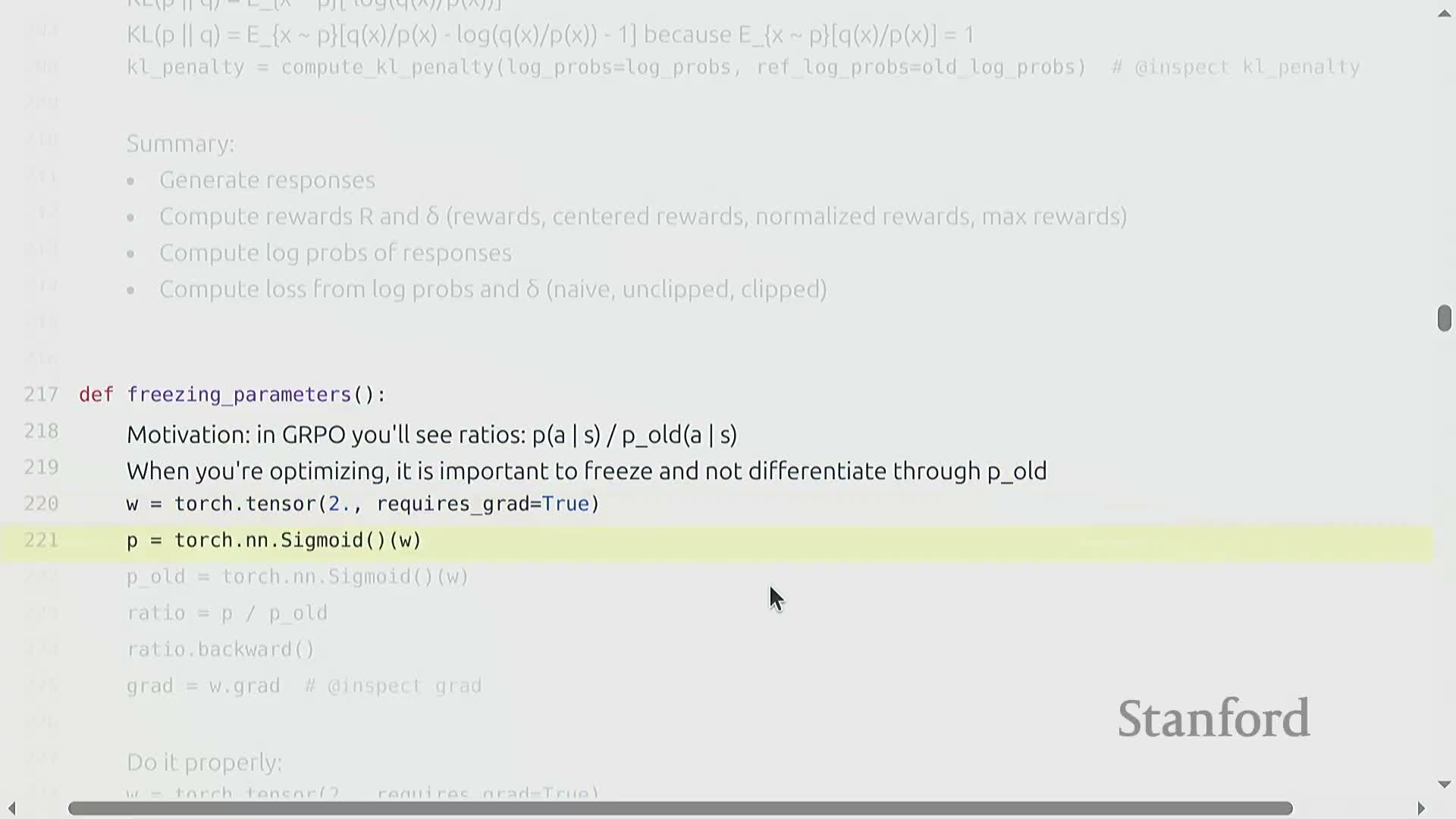
- Importance-weighted ratios (pi_theta / pi_old):
- Treat the denominator as a constant by disabling gradient flow through the old-policy computation.
- If you differentiate through both numerator and denominator, you can nullify gradients (e.g., ratio of identical parameterizations yields 1 and zero gradient), defeating learning.
- Treat the denominator as a constant by disabling gradient flow through the old-policy computation.
- Implementation guidance:
- Wrap old-policy log-probabilities or probabilities in no-grad contexts or cache scalar log-probabilities from a frozen checkpoint so the backward pass only propagates through the current policy.
- This engineering detail is critical for correctness when using PPO-style clipping or importance-weighted gradient estimators.
- Wrap old-policy log-probabilities or probabilities in no-grad contexts or cache scalar log-probabilities from a frozen checkpoint so the backward pass only propagates through the current policy.
Credit assignment and discounting considerations for outcome rewards
- Credit assignment challenges:
- Classical RL tools like discounting and bootstrapping are ambiguous when the reward is only available at episode end and many intermediate token decisions can matter.
- Discounting earlier tokens is not obviously beneficial because early strategic choices may determine later correctness more than later tokens themselves.
- Classical RL tools like discounting and bootstrapping are ambiguous when the reward is only available at episode end and many intermediate token decisions can matter.
- Practical approaches:
- Often smear credit across the entire response (broadcast final reward to all token positions).
- Or design process-level rewards if reliable intermediate signals exist.
- Often smear credit across the entire response (broadcast final reward to all token positions).
- Ongoing challenge:
- Designing effective credit-assignment mechanisms remains a core difficulty in sparse-reward LM tasks.
- Designing effective credit-assignment mechanisms remains a core difficulty in sparse-reward LM tasks.
GRPO clipped objective and KL regularization
-
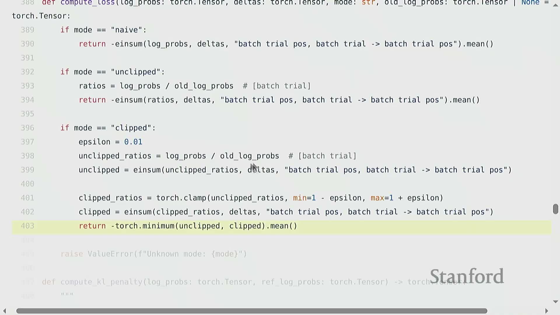
GRPO loss (group-relative, PPO-style):
- Compute importance-weighted ratios between current and old policies for sampled responses.
- Multiply ratios by deltas (reward/advantage variants).
-
Clip ratios to [1 − ε, 1 + ε] to bound update magnitudes and prevent destructive policy shifts.
- Take the minimum of the unclipped and clipped ratio-weighted deltas (with sign change to convert reward maximization into loss minimization).
- Compute importance-weighted ratios between current and old policies for sampled responses.
- Regularization:
- An auxiliary KL penalty between the current policy and a slowly updated reference policy provides additional stabilization.
- Unbiased but lower-variance estimators of KL are possible via algebraic rearrangement (e.g., q/p − log(q/p) − 1 forms).
- An auxiliary KL penalty between the current policy and a slowly updated reference policy provides additional stabilization.
- Purpose:
-
Clipping and KL regularization are practical mechanisms to stabilize policy updates in LM fine-tuning contexts.
-
Clipping and KL regularization are practical mechanisms to stabilize policy updates in LM fine-tuning contexts.
Algorithm components, inner/outer loop structure, and computational workflow
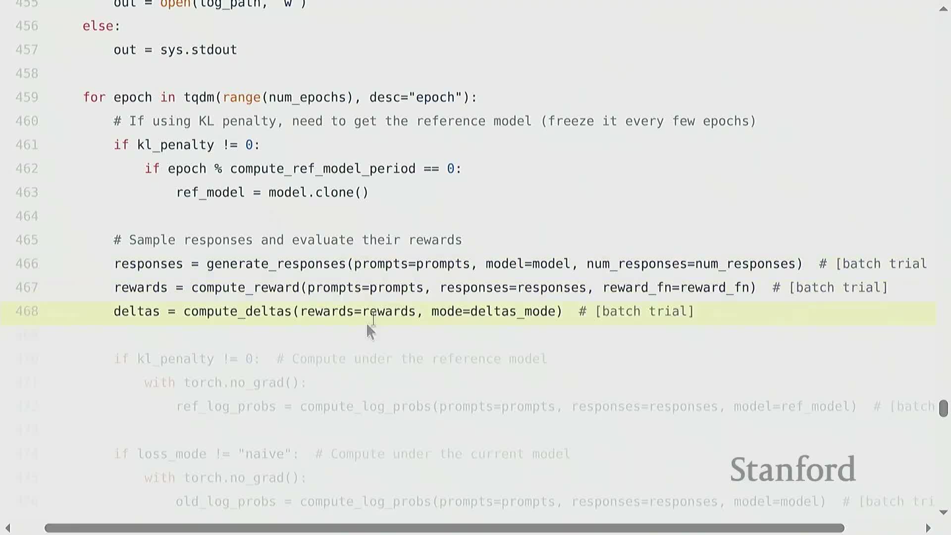
- Typical training loop structure:
- Outer loop: generate a fresh batch of responses (inference rollouts).
- Inner loop: perform multiple gradient steps on that static set of rollouts to amortize expensive sampling costs.
- Outer loop: generate a fresh batch of responses (inference rollouts).
- Key components:
-
Current policy being trained.
-
Frozen old policy used to compute importance ratios for clipping.
-
Slower-moving reference policy for KL regularization (updated less frequently).
-
Current policy being trained.
- Practical considerations:
- Cache log-probabilities from the rollout stage to avoid recomputing frozen-model outputs and reduce compute/memory needs.
- Architecting inference workers, checkpointing, and distributed pipelines is a major engineering concern beyond the scalar algorithmic choices.
- The inner/outer loop design reflects a trade-off between sample efficiency and inference cost at scale.
- Cache log-probabilities from the rollout stage to avoid recomputing frozen-model outputs and reduce compute/memory needs.
Why a separate KL reference vs. old policy and initialization considerations
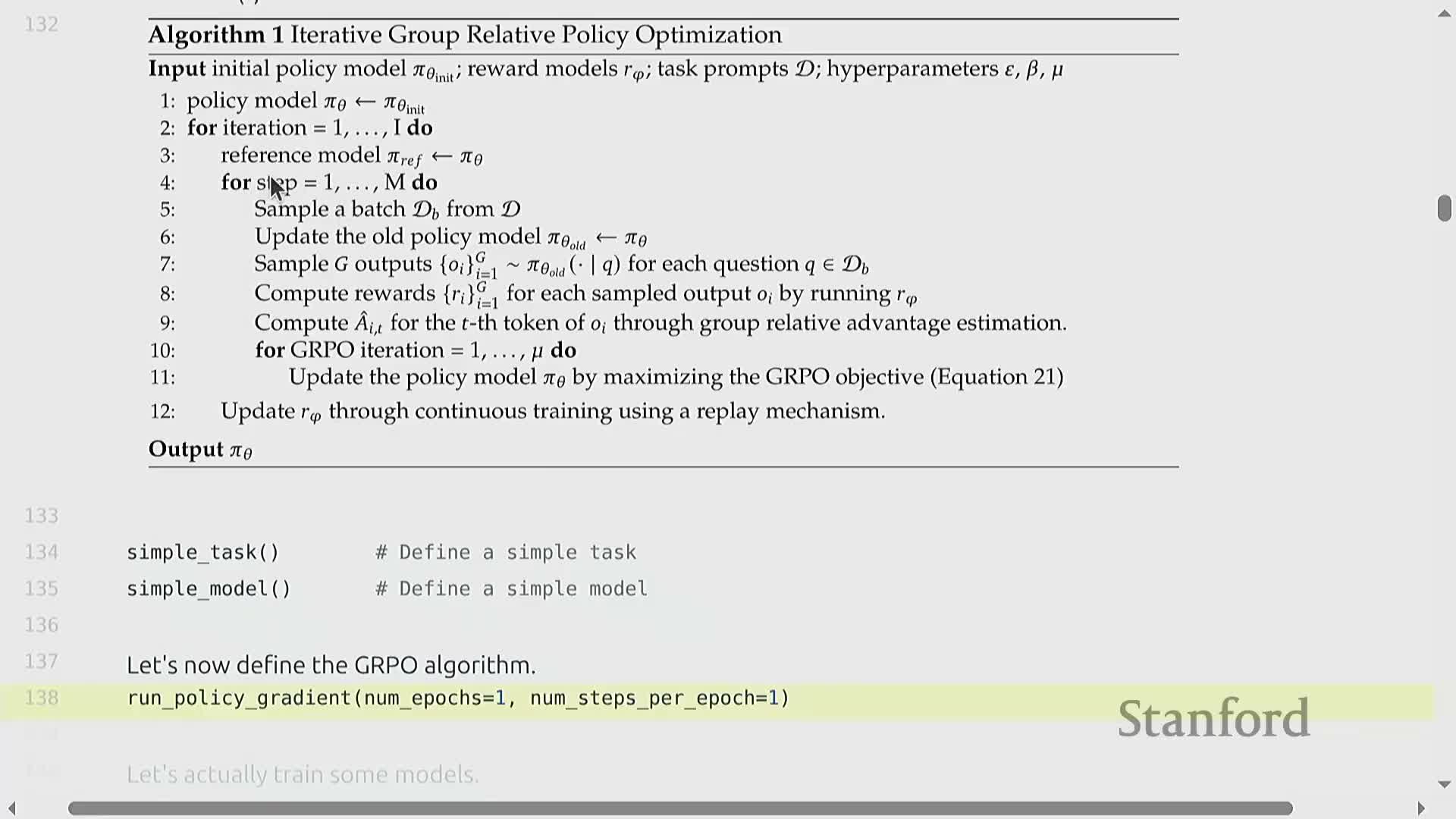
- Role of a slowly updated reference model for KL regularization:
-
Decouples the long-term regularization target from the short-term importance-ratio stabilization provided by the old policy.
- Helps define a stable optimization objective over inner-loop updates.
-
Decouples the long-term regularization target from the short-term importance-ratio stabilization provided by the old policy.
- Practical notes:
- If the KL target were the immediately previous policy (changing on the same timescale), regularization would shift too rapidly and could undermine convergence.
- Common practices: use a frozen checkpoint or periodic parameter copies as a constant regularization anchor; compute pi_old quantities from cached log-probabilities.
- Even when pi_old equals the current policy in initial iterations, valid updates occur because pi_old is treated as a constant in gradient computations.
- If the KL target were the immediately previous policy (changing on the same timescale), regularization would shift too rapidly and could undermine convergence.
Empirical sorting-task experiments and learning curve interpretation
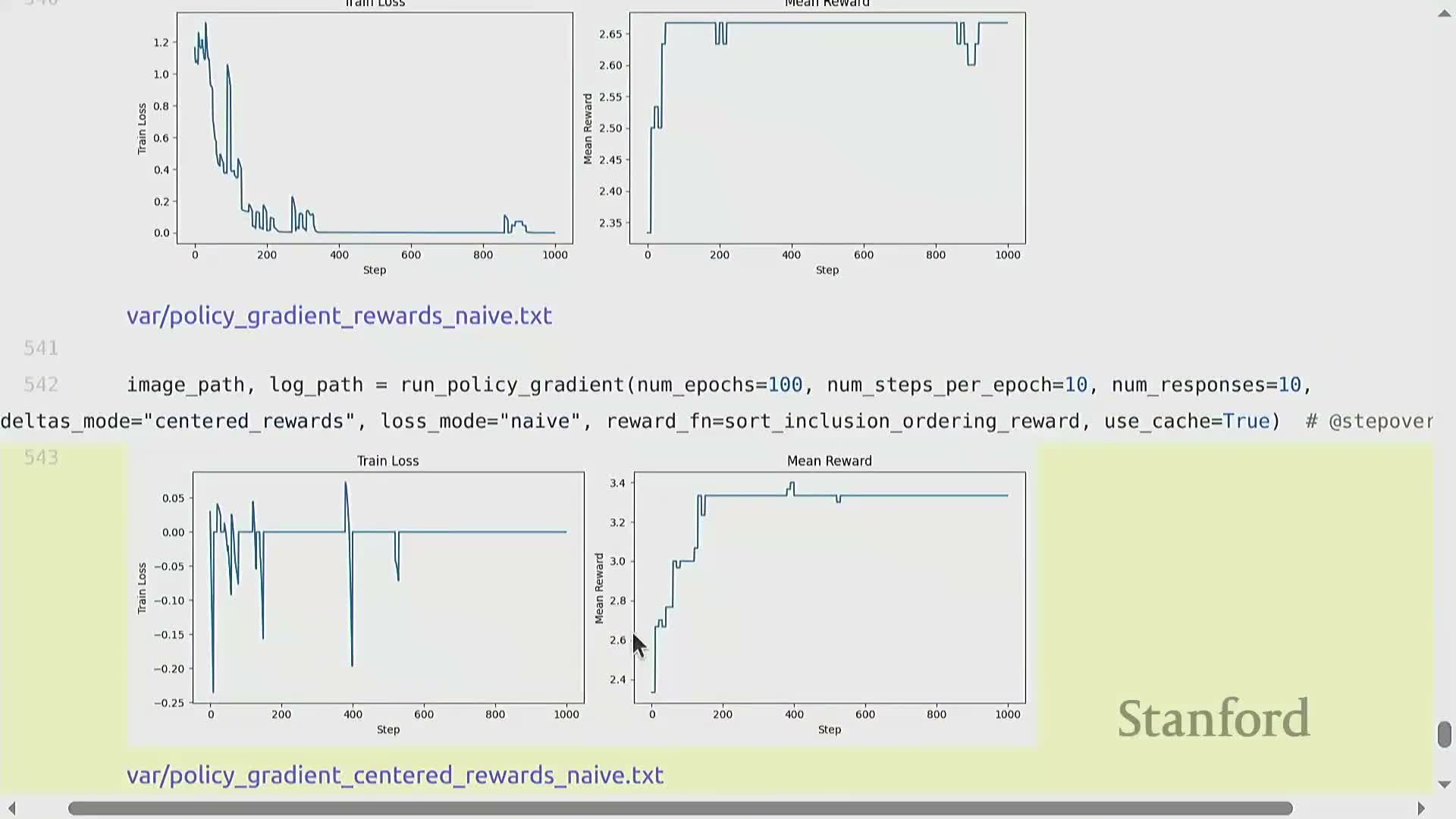
- Empirical observations on the toy sorting task:
-
Centered-reward updates often yield modest mean-reward improvements, pushing the policy away from lower-reward responses within a prompt cohort.
- Limitations:
- If all sampled responses for a prompt have identical rewards, centered deltas become zero and produce no update for that batch.
-
Loss curves can be misleading because the data distribution changes as the policy evolves.
- If all sampled responses for a prompt have identical rewards, centered deltas become zero and produce no update for that batch.
-
Centered-reward updates often yield modest mean-reward improvements, pushing the policy away from lower-reward responses within a prompt cohort.
- Monitoring recommendations:
- Track reward metrics on held-out prompts or regenerate rollouts to assess true progress.
- Experiments illustrate sensitivity to reward design, delta transformations, sampling variance, and the need for careful hyperparameter tuning.
- Track reward metrics on held-out prompts or regenerate rollouts to assess true progress.
Conclusions: promise of RL for LMs and scaling challenges
- Why use RL for LMs:
-
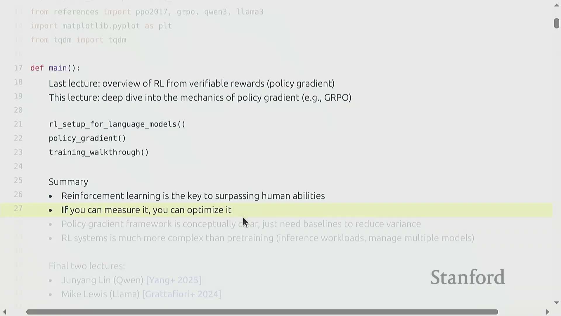
Optimizes behaviors that exceed imitation-limited supervised data by directly optimizing measurable objectives when verifiable rewards exist.
- Powerful for improving LM performance on tasks with quantifiable outcomes.
-
Optimizes behaviors that exceed imitation-limited supervised data by directly optimizing measurable objectives when verifiable rewards exist.
- Persistent challenges:
-
Sparse and delayed rewards.
- High variance in Monte Carlo estimators.
-
Reward-design vulnerabilities (hackability/exploitation).
- Complex credit assignment across long token sequences.
-
Sparse and delayed rewards.
- Systems-level complexity:
- Building scalable RL for LMs adds engineering burden beyond pretraining: inference cost, multi-model orchestration (policy, old policy, reference, reward models), and distributed execution must be managed.
- Building scalable RL for LMs adds engineering burden beyond pretraining: inference cost, multi-model orchestration (policy, old policy, reference, reward models), and distributed execution must be managed.
- Outlook:
- Continued research on reward specification, variance reduction, and system-level infrastructure is necessary to realize RL’s potential for large-scale language-model improvement.
- Continued research on reward specification, variance reduction, and system-level infrastructure is necessary to realize RL’s potential for large-scale language-model improvement.
Enjoy Reading This Article?
Here are some more articles you might like to read next: