The Foundations and Frontiers of Diffusion Models
(Work in progress I will gradually add more content when having more time:D Please stay tuned :D)
What are Diffusion Models?
Diffusion models are a class of generative models that generate data by progressively denoising a sample from pure noise. They are inspired by non-equilibrium thermodynamics and are based on a forward and reverse diffusion process:
- Forward Process (Diffusion Process): A data sample (e.g., an image) is gradually corrupted by adding Gaussian noise over multiple timesteps until it becomes nearly pure noise.
- Reverse Process (Denoising Process): A neural network learns to reverse this corruption by gradually removing noise step by step, reconstructing the original data distribution.
Analogy: Ink Dissolving in Water Imagine dropping a blob of ink into a glass of water:
- Forward process (Diffusion Process): Initially, the ink is concentrated in one place (structured data). Over time, it spreads out randomly, blending with the water (adding noise). Eventually, the entire glass becomes a uniformly colored mixture, losing its original structure (complete noise).
- Reverse process (Denoising Process): If we had a way to perfectly reverse time, we could watch the ink particles retrace their paths, reassembling into the original drop (generating the original data from noise). Diffusion models learn to perform this “reverse process” step by step using machine learning.
Non-Equilibrium Thermodynamics
Thermodynamics studies how energy moves and changes in a system. In equilibrium thermodynamics, systems are in balance—nothing is changing. Non-equilibrium thermodynamics, on the other hand, deals with systems that are constantly evolving, moving between states of disorder and order.
In diffusion models, the forward process (adding noise to data) and the reverse process (removing noise) resemble a non-equilibrium thermodynamic system because they describe an evolving state that moves from order (structured data) to disorder (pure noise) and back to order (reconstructed data).
Brownian Motion
Brownian motion describes the random movement of tiny particles (like pollen grains in water) due to collisions with molecules. This randomness is similar to how noise is added in diffusion models.
Advantages of Diffusion Models and the Trade-offs
Diffusion models offer several key advantages over traditional generative models like GANs and VAEs:
-
High-Fidelity Samples: Unlike VAEs and GANs which generate samples in one step, diffusion models create samples gradually by denoising. This step-by-step process allows the model to first establish coarse image structure before refining fine details, resulting in higher quality outputs.
-
Training Stability: Diffusion models are easier to train compared to GANs as they use a single tractable likelihood loss. They don’t suffer from training instabilities like mode collapse that often plague GANs.
-
Sample Diversity: Similar to VAEs, diffusion models maximize likelihood which ensures coverage of all modes in the training dataset. This leads to more diverse outputs compared to GANs which can suffer from mode collapse.
-
Guidance Ability: The generation process of Diffusion models can be guided by external conditions, such as text prompts, images, or other modalities. While the conditional generation can also be possible with VAEs or GANs, the guidance ability of Diffusion models is more flexible, thanks to (1) the multi-step nature of the generation process, that can generate samples in a coarse-to-fine manner, and (2) the separable between the control signal (through the cross-attention layers) and the data diversity (through prior Gaussian distribution), making the concept space more detachable from the data manifold. You can unlearn (machine unlearning) a specific concept or inject a new concept (personalization) without hurting too much the other concepts or changing model architecture.
However, diffusion models still have some trade-offs, but have been greatly mitigated by the massive research efforts in the community.
The main trade-off is generation speed - diffusion models require multiple neural network passes to generate samples, making them slower than single-pass models like GANs and VAEs. However, various sampling optimization techniques have been developed to significantly reduce this computational overhead, such as Diffusion Distillation or Consistency Models, that can generate samples even in a single step.
Another trade-off is the training complexity, as it requires to cover all diffusion steps to train the model, which is multiple times expensive than training a single-step model.
A Brief History of Diffusion Models and Their Variants
Before diffusion models took over, the field of generative modeling was dominated by two major families: VAEs and GANs, where their glory era spans from 2014 until 2020.
Variational Autoencoders (VAEs), introduced by Kingma and Welling (2013), were the first deep generative models with a solid probabilistic foundation. They use variational inference and the reparameterization trick to learn a latent space that allows smooth interpolation and sampling:
\[z \sim q_\phi(z|x), \quad x \sim p_\theta(x|z)\]VAEs are elegant and interpretable, but their samples often appeared blurry due to the Gaussian decoder assumption.
Generative Adversarial Networks (GANs), proposed by Goodfellow et al. (2014), took a completely different path — framing generation as a two-player game between a generator \(G\) and discriminator \(D\):
\[\min_G \max_D \; \mathbb{E}_{x \sim p_{\text{data}}}[\log D(x)] + \mathbb{E}_{z \sim p(z)}[\log (1 - D(G(z)))]\]GANs quickly dominated image generation, producing strikingly sharp and realistic results. Yann LeCun famously called GANs “the most interesting idea in the last 10 years in machine learning.”
However, GANs were notoriously hard to train (mode collapse, instability), and VAEs struggled with sample quality.
The Roots: Score-Based Generative Modeling
The foundation of diffusion models lies in score-based generative modeling, which began with Hyvärinen, Aapo, and Peter Dayan. “Estimation of non-normalized statistical models by score matching.” in 2005, where the first time proposed the score matching loss to estimate the score function \(\nabla_x \log p(x)\) of the data distribution rather than modeling the data distribution \(p(x)\) directly.
\[\mathcal{L}_{ScoreMatching}(\theta) = \mathbb{E}_{x} \left[ \| s_\theta(x) - \nabla_x \log p(x) \|^2 \right]\]This idea shifted focus from learning explicit probabilities to learning how to move data toward higher density regions.
Denoising Score Matching (DSM)
Building on this, Vincent (2011) proposed Denoising Score Matching (DSM), observing that learning from noisy data is more stable.
By perturbing the data with a known noise distribution, and then learning how to reverse the noise to get the clean data, the goal now is to estimate the score function \(\nabla_x \log p(x)\) from the noisy data.
where \(q(x_t \mid x_0)\) is the noise distribution, and \(x_0\) is the clean data. This denoising process later becomes the core mechanism of modern diffusion models.
Diffusion Probabilistic Models (Sohl-Dickstein et al., 2015)
Sohl-Dickstein et al., 2015 – “Deep Unsupervised Learning using Nonequilibrium Thermodynamics” introduced Diffusion Probabilistic Models (DPM), inspired by nonequilibrium thermodynamics, with forward diffusion process gradually adding Gaussian noise to the data, and reverse diffusion process learns to denoise step by step. This was the first formalization of iterative denoising as generation. However, at the time, these models did not work well on large-scale datasets and did not get much attention from the community.
The Modern Rebirth: DDPM (Ho, Jain, Abbeel, 2020)
Diffusion Models rebirth in 2020 with the introduction of DDPM (Denoising Diffusion Probabilistic Models) (Ho, Ajay, Abbeel) at NeurIPS 2020, reintroducing and refining Sohl-Dickstein’s idea with modern deep learning tools. Crucial improvements include simplified training objective equivalent to denoising score matching, reparameterization trick to predict the noise using a neural network, and demonstration on large-scale datasets with high-quality image comparable to GANs.
One year earlier, at NeurIPS 2019, Song and Ermon also reintroduced the idea of Hyvärinen et al., 2005 and Vincent 2011, with a novel sampling algorithm called Langevin Dynamics that allows to sample from the data distribution using the score function.
\[x_{t-1} = x_t + \epsilon \nabla_x \log p_{t}(x_t) + \sqrt{2\epsilon} z\]where \(\epsilon\) is a small positive constant and \(z \sim \mathcal{N}(0, I)\) is a standard Gaussian noise.
The Unified View: Score-Based SDEs (Song et al., 2021)
At ICLR 2021, Song et al. introduced
“Score-Based Generative Modeling through Stochastic Differential Equations”,
which unified all previous methods — score matching, DDPM, and DDIM — under one continuous-time framework.
They showed that diffusion models correspond to solving an SDE:
\[dx_t = f(x_t, t)\,dt + g(t)\,dw_t\]and its reverse-time counterpart uses the learned score ( \nabla_x \log p_t(x) ).
This framework established that:
- DDPM is a discrete stochastic version.
- DDIM is a deterministic ODE version.
- Score-based models are equivalent up to reparameterization.
Diffusion models succeeded where VAEs were blurry and GANs were unstable. They combined the best of both worlds - the training stability of VAEs and the sample quality of GANs. Together, these advances reshaped the landscape of generative modeling — leading to today’s foundation models like Stable Diffusion and DALL·E 3, which trace their roots back to score matching in 2005.
Mathematical Foundation
Diffusion models are built on a deep interplay between differential equations, probability theory, and variational inference. To understand why the model works, we need to trace how these ideas connect: from describing how systems evolve over time, to modeling probability densities, to designing trainable objectives. While it seems complicated at first glance, the more I dive into it, the more I realize the beauty and elegance of Diffusion Models.
Differential Equations: ODEs and SDEs
We start with ordinary differential equations (ODEs), which describe how a system changes deterministically over time based on its current state.
\[\frac{dx}{dt} = f(x, t)\]where \(x(t)\) is the state of the system - the function we want to solve -and \(t\) is time. \(f(x, t)\) defines how \(x\) changes over time.
This is a useful starting point, but in real-world data generation, we must account for randomness. That brings us to stochastic differential equations (SDEs), which incorporate random fluctuations into the system.
\[dx = f(x, t) dt + g(x, t) dW_t\]where the drift term \(f(x, t) dt\) captures the deterministic trends, while the diffusion term \(g(x, t) dW_t\) captures the random fluctuations via a Wiener process \(W_t\).
👉 Motivation: Diffusion models inject noise step by step, so SDEs provide the natural language to describe this stochastic corruption process. More specifically, the drift term \(f(x, t)\) is the shift of the mean of the distribution, and the diffusion term \(g(x, t)\) is the spread of the distribution - injecting Gaussian noise.
Forward and Reverse Diffusion Processes
Forward Process (Adding Noise)
The forward diffusion process transform a data sample \(x_0\) into pure noise \(x_T\) over time:
\[dx = f(x, t)dt + g(t) dW_t\]Intuitively, the drift term \(f(x, t) dt\) shifts the mean of the distribution by a deterministic amount \(f(x,t)\) (i.e., is a function of \(x\) and current time \(t\)) to a zero mean distribution. The diffusion term \(g(t) dW_t\) spreads the distribution by injecting Gaussian noise, increasing the variance of the distribution.
Note that \(g(t)\) is a function of current time \(t\) only, to guarantee that each noised distribution remains Gaussian with a know mean and variance. This make the forward process to be simple and tractable, that we can have exact sampling formula for each specific time step \(t\), i.e., \(q (x_t \mid x_0) = \mathcal{N}(x_t; \sqrt{\bar{\alpha}_t} x_0, (1-\bar{\alpha}_t)I)\).
Reverse Process (Removing Noise) In order to generate data from pure noise \(x_T\), we need to reverse the diffusion process by Reverse-Time SDE (Anderson 1982).
\[dx = \left[ f(x,t) - \frac{1}{2} g^2(t) \nabla_x \log p_t(x) \right] dt + g(t) d\tilde{W}_t\]where \(\nabla_x \log p_t(x)\) is the score function, which estimates the structure of data at time \(t\) - how likely different data points are at each step. \(d\tilde{W}_t\) is another Wiener process but in the reverse direction.
👉 Motivation: Since \(f(x,t)\) and \(g(t))\) are known, to reverse noise, we must know the score function. So we train a neural network to approximate the score function \(\nabla_x \log p_t(x)\). This is the core of the diffusion model.
Euler Method for Numerical Integration
To simulate the reverse process, we need a numerical method to integrate the SDE backward through time. The Euler–Maruyama method (a stochastic generalization of the Euler method) provides a simple, first-order approximation.
For the variance-preserving (VP) SDE used in diffusion models, the deterministic part of the reverse process (ignoring noise sampling) can be expressed as an ODE:
\[\frac{dx}{dt} = f(x,t) - \frac{1}{2} g^2(t) \nabla_x \log p_t(x)\]Now, using the Euler method to integrate this ODE backward in time from \(t_{n+1}\) to \(t_n\):
\[x_{t_n} = x_{t_{n+1}} + (t_{n+1} - t_{n}) \frac{dx}{dt} \bigg|_{x=x_{t_{n+1}}, t=t_{n+1}}\]Substituing the ODE into the Euler method, we get:
\[x_{t_n} = x_{t_{n+1}} + (t_{n+1} - t_{n}) \left[ f(x_{t_{n+1}}, t_{n+1}) - \frac{1}{2} g^2(t_{n+1}) \nabla_x \log p_{t_{n+1}}(x_{t_{n+1}}) \right]\]This stepwise update forms the foundation of diffusion sampling algorithms like DDPM and DDIM, where the score term is replaced by the neural network’s prediction.
Implementation of the Euler method
In the context of consistency models, the update rule is derived from the Probability Flow ODE (PF-ODE):
\[\frac{dx}{dt} = -t s_{\phi}(x,t)\]where \(s_{\phi}(x,t)\) is a learned score function related to the model output \(f_{\theta}(x,t)\). From the definition of the consistency function (please refer to the Consistency Models section), we have:
\[s_{\phi}(x,t) = \frac{x - f_{\theta}(x,t)}{t^2}\]Substituing this into the PF-ODE Euler update:
\[\hat{x}_{t_n} = x_{t_{n+1}} - (t_n - t_{n+1}) t_{n+1} s_{\phi}(x_{t_{n+1}}, t_{n+1})\]We get: \(\hat{x}_{t_n} = x_{t_{n+1}} - (t_n - t_{n+1}) \frac{x - f_{\theta}(x,t)}{t}\)
This formula defines a single-step explicit Euler integration: it can predict the next step \(x_{t_n}\) from the current step \(x_{t_{n+1}}\).
Python implementation:
@th.no_grad()
def euler_solver(samples, t, next_t, x0):
    x = samples
    if teacher_model is None:
        denoiser = x0
    else:
        denoiser = teacher_denoise_fn(x, t) # f_{\theta}(x,t) - consistency model output
    d = (x - denoiser) / append_dims(t, dims)
    samples = x + d * append_dims(next_t - t, dims)

    return samples
👉 Interpretation:
-
dis the difference between the current step and the next step. -
next_t - tis the time step size (negative for reverse time integration). - The Euler method uses only the slope at the start of the interval, making it simple but potentially less accurate for large steps.
Heun Method (Improved Euler / Predictor–Corrector)
The Heun method is a second-order numerical scheme that improves on Euler by estimating the derivative twice — at the beginning and at the end of the time interval — and then averaging them. This yields better stability and smaller integration error, especially for stiff or nonlinear dynamics like those in diffusion models.

The update consists of two stages:
- Predictor (Euler step):
where \(d_{t_{n+1}} = \frac{x_{t_{n+1}} - f_{\theta}(x_{t_{n+1}}, t_{n+1})}{t_{n+1}}\).
- Corrector (Second-order correction): Evaluate a new derivative \(d_{t_n}\) at the predicted point \(\tilde{x}_{t_n}\), then update the final point:
@th.no_grad()
def heun_solver(samples, t, next_t, x0):
    x = samples
    if teacher_model is None:
        denoiser = x0
    else:
        denoiser = teacher_denoise_fn(x, t) # f_{\theta}(x,t) - consistency model output


    # IMPORTANT - Euler method
    d = (x - denoiser) / append_dims(t, dims)
    samples = x + d * append_dims(next_t - t, dims)
    if teacher_model is None:
        denoiser = x0
    else:
        denoiser = teacher_denoise_fn(samples, next_t) # f_{\theta}(x,t) - consistency model output

    next_d = (samples - denoiser) / append_dims(next_t, dims)
    samples = x + (d + next_d) * append_dims((next_t - t) / 2, dims)

    return samples
Fokker-Planck Equation: From Trajectories to Distributions
SDEs describe how the distribution of a system changes over time, but what about the distribution of data as noise accumulates? The Fokker-Planck equation bridges the gap between trajectories and distributions, explaining how noise pushes data distributions \(p_t(x)\) toward isotropic Gaussian distributions.
\[\frac{\partial p_t(x)}{\partial t} = -\nabla_x \cdot (f(x,t) p_t(x)) + \frac{1}{2} \nabla_x \cdot (g(t)^2 \nabla_x p_t(x))\]where \(p_t(x)\) is the distribution of the data at time \(t\).
The first term \(-\nabla_x \cdot (f(x,t) p_t(x))\) describes the change of the probability density \(p_t(x)\) with the drift term \(f(x,t)\) (as the velocity of that mass). The divergence operator \(\nabla_x \cdot\) measures how much the mass is spreading out (positive divergence) or converging/concentrating (negative divergence) at any given point \(x\). The whole term \(- \nabla_x \cdot (f(x,t) p_t(x))\) describes a rate of change of the probability density \(p_t(x)\) at any given point \(x\), where the positive value means the mass is flowing away from \(x\), causing \(p_t(x)\) to decrease (hence the negative sign), and vice versa.
The second term \(\frac{1}{2} \nabla_x \cdot (g(t)^2 \nabla_x p_t(x))\) presents the spreading and smoothing effect of the probability density \(p_t(x)\) over time due to the influence of the random fluctuations. More specifically, \(g(t)\) controls the magnitude of the random noise. The \(\nabla_x p_t(x)\) term describes the steepness or slope of \(p_t(x)\) at any given point \(x\). The whole term \(\frac{1}{2} \nabla_x \cdot (g(t)^2 \nabla_x p_t(x))\) describes a rate of change of the probability density \(p_t(x)\), i.e., the larger the gradient, the more the density rising sharply around \(x\). Similar to the first term, \(\nabla_x \cdot\) measures how much the mass is spreading out (positive divergence) or converging/concentrating (negative divergence) at any given point \(x\) with two differences:
- It contains the random fluctuations term \(g(t)^2\) instead of the drift term \(f(x,t)\), introducing randomness into the system.
- It proportional to the gradient \(\nabla_x p_t(x)\), meaning that the slope/sharp region is more affected/spread out than the flat region (which has smaller gradient \(\nabla_x p_t(x)\)).
Score Matching and Denoising
Since the reverse SDE depends on the score function \(\nabla_x \log p_t(x)\) (which is intractable), we need to design a training objective to approximate this function. Vincent et al. proposed denoising score matching (Vincent 2011) to approximate by training a neural network \(s_{\theta}(x_t, t)\) to approximate the conditional score function \(\nabla_x \log q(x_t \mid x_0, \epsilon)\) (where \(q\) is a tractable forward process, \(dx = f(x, t)dt + g(t)dW_t\)) assuming that \(q(x_t \mid x_0) \approx p_t(x_t)\) at time \(t\) (which is a reasonable assumption).
This objective aims to minimize the difference:
\[\mathbb{E}_{p(x_0), \epsilon \sim \mathcal{N}(0, I)} \left[ \left\| s_{\theta}(x_t, t) - \nabla_x \log p_t(x_t \mid x_0, \epsilon) \right\|^2 \right]\]Variational Perspective and KL Minimization
Another way to frame diffusion models is to consider them as a variational inference problem. The forward process \(q(x_{0:T})\) is a know noising chain of distributions, and the reverse process \(p_{\theta}(x_{0:T})\) is learned. Therefore, we can use the variational lower bound (ELBO) to train the model.
\[\mathbb{E}_{q(x_{0:T})} \left[ D_{KL} \left( q(x_{t-1} \mid x_t, x_0) \parallel p_{\theta}(x_{t-1} \mid x_t) \right) \right]\]ELBO
Evidence lower bound (ELBO) is a key concept in variational inference, which is used in VAEs to approximate the log-likelihood of the data.
Let \(X\) and \(Z\) be random variables, jointly distributed with distribution \(p_\theta\). For example, \(p_\theta(X)\) is the marginal distribution of \(X\), and \(p_\theta(Z \mid X)\) is the conditional distribution of \(Z\) given \(X\). Then, for a sample \(x \sim p_{\text{data}}\), and any distribution \(q_\phi\), the ELBO is defined as
\[L(\phi, \theta; x) := \mathbb{E}_{z\sim q_\phi(\cdot|x)} \left[\ln \frac{p_\theta(x,z)}{q_\phi(z|x)}\right].\]The ELBO can equivalently be written as
\[\begin{aligned} L(\phi, \theta; x) &= \mathbb{E}_{z\sim q_\phi(\cdot|x)}[\ln p_\theta(x,z)] + H[q_\phi(z \mid x)] \\ &= \ln p_\theta(x) - D_{KL}(q_\phi(z \mid x) || p_\theta(z \mid x)). \end{aligned}\]In the first line, \(H[q_\phi(z \mid x)]\) is the entropy of \(q_\phi\), which relates the ELBO to the Helmholtz free energy. In the second line, \(\ln p_\theta(x)\) is called the evidence for \(x\), and \(D_{KL}(q_\phi(z \mid x) \mid\mid p_\theta(z \mid x))\) is the Kullback-Leibler divergence between \(q_\phi\) and \(p_\theta\). Since the Kullback-Leibler divergence is non-negative, \(L(\phi, \theta; x)\) forms a lower bound on the evidence (ELBO inequality)
\[\ln p_\theta(x) \geq \mathbb{E}_{z\sim q_\phi(\cdot|x)}\left[\ln \frac{p_\theta(x,z)}{q_\phi(z|x)}\right].\]Deep-dive topics about VAE might including:
- Reparameterization Trick: How to sample from a distribution in a differentiable way - Wiki
- The problem of KL divergence: mode seeking vs mode covering by Andy Jones
- A nice property of VAEs: Disentanglement Representation Learning
Tweedie’s formula
Finally, Tweedie’s formula gives a neat probabilistic justification for the denoising score matching objective:
\[\mathbb{E} [ x_0 \mid x_t] = x_t + \sigma_t^2 s_{\theta}(x_t, t)\]where \(s_{\theta}(x_t, t)\) is the score function to be learned by the neural network. It shows that the posterior mean of clean data given a noisy data is just the noisy sample plus a correction term proportional to the score function.
In some papers such as ESD (Gandikota et al. 2023), where we need to fine-tune the pretrained model and match the score function of the original and the fine-tuned model, they use Tweedie’s formula to justify the matching term.
Variants of Diffusion Models
The original formulation of diffusion models can be implemented in several ways. Two of the most influential variants are Denoising Diffusion Probabilistic Models (DDPMs) and Denoising Diffusion Implicit Models (DDIMs). Both share the same forward noising process but differ in how they perform the reverse (denoising) process during inference.
DDPM
DDPM (Ho et al. 2020) is the classic diffusion model:
- The Reverse process is defined as a Markov chain, where each step \(x_t \to x_{t-1}\) involves sampling from a Gaussian distribution conditioned on \(x_t\).
- Sampling os stochastic, even with the same starting noise \(x_T\), the generated data \(x_0\) is different.
- While highly effective and stable (compared to GANs), DDPMs require hundreds to thousands of steps to slowly add/remove noise, which makes inference slow.
Read more about DDPM in another blog post here
DDIM
DDIM (Song et al. 2020) builds on DDPM but introduces a non-Markovian reverse process, enabling faster sampling. It also allows us to use the same training process as DDPM, e.g., we can use pretrained DDPM models to generate data.
The sampling process of DDIM is as follows:
\[x_{t-1} = \sqrt{\alpha_{t-1}} \left(\frac{x_t - \sqrt{1-\alpha_t}\epsilon_\theta^{(t)}(x_t)}{\sqrt{\alpha_t}}\right) + \sqrt{1-\alpha_{t-1}-\sigma_t^2} \cdot \epsilon_\theta^{(t)}(x_t) + \sigma_t\epsilon_t\]where the first term represents the “predicted \(x_0\)”, the second term is the “direction pointing to \(x_t\)”, and the last term is random noise.
By setting \(\sigma_t = 0\) for all \(t\), DDIM becomes a deterministic process given \(x_{t-1}\) and \(x_0\), except for \(t=1\). In other words, the intermediate steps \(x_{T-1}, x_{T-2}, \ldots, x_1\) are deterministic given starting noise \(x_T\).
Read more about DDIM in another blog post here
Score Matching
Score-based generative models (Song and Ermon 2019, Song et al. 2021(published in ICLR 2021, are a family of generative models that learn to estimate the score function — the gradient of the log-density of the data distribution \(s_\theta(x, t) \approx \nabla_x \log p_t(x)\). Intuitively, the score function tells us which direction in the input space increases the likelihood of the data. By learning this function at different noise levels (at different time steps \(t\)), the model learns how to denoise a sample toward realistic data.
Training Objective
The ideal objective of score matching is:
\[\min_{\theta} \mathbb{E}_{p_t(x)} \left[ \| s_\theta(x, t) - \nabla_x \log p_t(x) \|^2 \right]\]which can be shown to be equivalent to
\[\min_{\theta} \mathbb{E}_{p_t(x)} \left[ \text{trace}(\nabla_x s_{\theta}(x, t)) + \frac{1}{2} \| s_{\theta}(x, t) \|^2 \right]\]With deep networks and high-dimensional data, it is difficult to obtain the expectation over the data distribution, especially with the \(\text{trace}(\nabla_x s_{\theta}(x, t))\).
One of the popular ways to overcome this is to use Denoising Score Matching (DSM) (Vincent 2011). The idea is first to perturbs the data \(x\) with a known Gaussian noise process \(q(x_t \mid x_0)\), then train the score network \(s_\theta(x_t, t)\) to denoise the perturbed data \(x_t\) back to the original data \(x_0\).
\[\min_{\theta} \mathbb{E}_{q(x_t \mid x), p_t(x)} \left[ \| s_\theta(x_t, t) - \nabla_{x_t} \log q(x_t \mid x) \|^2 \right]\]For Gaussian perturbations:
\[\nabla_{x_t} \log q(x_t \mid x) = -\frac{x_t - \alpha_t x_0}{\sigma_t^2}\]Hence, we can train \(s_\theta(x_t, t)\) to match this target directly.
Sampling
In Song and Ermon 2019, they use Langevin dynamics to samples data with the score function \(s_\theta(x, t)\). Given a fixed step size \(\epsilon\), and an inital value \(x_T \sim \mathcal{N}(0, I)\), the Langevin dynamics recursively update the data as follows:
\[x_{t-1} = x_t + \frac{\epsilon}{2} s_{\theta}(x_t, t) + \sqrt{\epsilon} z_t\]where \(z_t \sim \mathcal{N}(0, I)\).
\(\epsilon\)-prediction
Instead of predicting the score directly, DDPM variants predict the noise \(\epsilon\) added to the data, which is equivalent to predicting the score but more numerically stable.
The data corruption process is:
\[x_t = \sqrt{\bar{\alpha}_t} x_0 + \sqrt{1 - \bar{\alpha}_t} \epsilon\]Then the score function relates to the noise predictor as:
\[s_\theta(x_t, t) = -\frac{\epsilon_{\theta}(x_t, t)}{\sqrt{1 - \bar{\alpha}_t}}\]The training loss becomes:
\[\mathcal{L}_{DDPM}(\theta) = \mathbb{E}_{t, x_0, \epsilon} \left[ \| \epsilon_\theta(x_t, t) - \epsilon \|^2 \right]\]From DDPM to Score Matching
It can be seen that the key idea of both DDPM and SMLD is to perturb the data with a known noise distribution, and then denoise back to the original data. In the following work (Song et al. 2021), the authors unified the two frameworks into a single framework called Score Matching, with an infinite number of noise scales.
First, the diffusion process can be defined as a SDE:
\[dx = f(x, t) dt + g(t) dW_t\]where \(f(x, t)\) is the drift term and \(g(t)\) is the diffusion term and \(W_t\) is the Wiener process.
The reverse diffusion process, which denoises the data from \(x_T \sim \mathcal{N}(0, I)\) to \(x_0 \sim p(x)\), can be defined as a reverse-time SDE:
\[dx = [f(x, t) - g(t)^2 \nabla_x \log p_t(x)] dt + g(t) d\bar{W}_t\]where \(\bar{W}_t\) is the reverse-time Wiener process.
Different diffusion model families have different choices of \(f(x, t)\) and \(g(t)\):
- Variance Exploding (VE) SDE: \(f(x, t) = 0, g(t) = \sqrt{\frac{d\sigma_t^2}{dt}}\) as in SMLD
- Variance Preserving (VP) SDE: \(f(x, t) = -\frac{1}{2}\beta_t x, g(t) = \sqrt{\beta_t}\) as in DDPM
Sampling with the Euler-Maruyama method
Once trained, the score network defines the reverse-time dynamics that transform Gaussian noise \(x_T \sim \mathcal{N}(0, I)\) to the data sample \(x_0 \sim p(x)\). We can simulate the reverse SDE numerically using the Euler-Maruyama method:
\[x_{t-1} = x_t + (t_n - t_{n+1}) \frac{dx}{dt} \big| _{x=x_t, t = t_n}\] \[x_{t-1} = x_t + (t_n - t_{n+1}) \left[ f(x_t, t_n) - g(t_n)^2 \nabla_x \log p_{t_n}(x_t) \right] + g(t_n) \sqrt{t_n - t_{n+1}} z_t\]where \(z_t \sim \mathcal{N}(0, I)\).
This adds both a deterministic drift (using the learned score function) and a stochastic noise term to preserve the sample diversity.
If we remove the noise term (set \(z_t = 0\)), we obtain the Probability Flow ODE, a deterministic trajectory equivalent in distribution to the reverse-time SDE, which is the foundation of DDIM deterministic sampling.
Implementation of Score Matching
The official implementation of Score Matching is https://github.com/yang-song/score_sde_pytorch.
In Diffusers lib, the Score SDV VP and VE schedulers can be found here and here.
Notable functions/methods in the official implementation (PyTorch version):
  def discretize(self, x, t):
    """Discretize the SDE in the form: x_{i+1} = x_i + f_i(x_i) + G_i z_i.

    Useful for reverse diffusion sampling and probabiliy flow sampling.
    Defaults to Euler-Maruyama discretization.

    Args:
      x: a torch tensor
      t: a torch float representing the time step (from 0 to `self.T`)

    Returns:
      f, G
    """
    dt = 1 / self.N
    drift, diffusion = self.sde(x, t)
    f = drift * dt
    G = diffusion * torch.sqrt(torch.tensor(dt, device=t.device))
    return f, G
  def reverse(self, score_fn, probability_flow=False):
    """Create the reverse-time SDE/ODE.

    Args:
      score_fn: A time-dependent score-based model that takes x and t and returns the score.
      probability_flow: If `True`, create the reverse-time ODE used for probability flow sampling.
    """
    N = self.N
    T = self.T
    sde_fn = self.sde
    discretize_fn = self.discretize

    # Build the class for reverse-time SDE.
    class RSDE(self.__class__):
      def __init__(self):
        self.N = N
        self.probability_flow = probability_flow

      @property
      def T(self):
        return T

      def sde(self, x, t):
        """Create the drift and diffusion functions for the reverse SDE/ODE."""
        drift, diffusion = sde_fn(x, t)
        score = score_fn(x, t)
        drift = drift - diffusion[:, None, None, None] ** 2 * score * (0.5 if self.probability_flow else 1.)
        # Set the diffusion function to zero for ODEs.
        diffusion = 0. if self.probability_flow else diffusion
        return drift, diffusion

      def discretize(self, x, t):
        """Create discretized iteration rules for the reverse diffusion sampler."""
        f, G = discretize_fn(x, t)
        rev_f = f - G[:, None, None, None] ** 2 * score_fn(x, t) * (0.5 if self.probability_flow else 1.)
        rev_G = torch.zeros_like(G) if self.probability_flow else G
        return rev_f, rev_G

    return RSDE()
IMPORTANT NOTE: For models trained with VP SDE, the marginal distribution of \(x_t\) given clean data \(x_0\) is Gaussian: \(x_t \sim \mathcal{N}(\sqrt{\bar{\alpha}_t} x_0, \sigma_t^2 I)\) or in general SDE notation: \(x_t = \text{mean}(x_0, t) + \text{std}(t) \dot z\) where \(z \sim \mathcal{N}(0, I)\).
Therefore, when training, we sample
mean, std = sde.marginal_prob(batch, t)
perturbed_data = mean + std * z
class VPSDE(SDE):
  def __init__(self, beta_min=0.1, beta_max=20, N=1000):
    """Construct a Variance Preserving SDE.

    Args:
      beta_min: value of beta(0)
      beta_max: value of beta(1)
      N: number of discretization steps
    """
    super().__init__(N)
    self.beta_0 = beta_min
    self.beta_1 = beta_max
    self.N = N
    self.discrete_betas = torch.linspace(beta_min / N, beta_max / N, N)
    self.alphas = 1. - self.discrete_betas
    self.alphas_cumprod = torch.cumprod(self.alphas, dim=0)
    self.sqrt_alphas_cumprod = torch.sqrt(self.alphas_cumprod)
    self.sqrt_1m_alphas_cumprod = torch.sqrt(1. - self.alphas_cumprod)

  @property
  def T(self):
    return 1

  def sde(self, x, t):
    beta_t = self.beta_0 + t * (self.beta_1 - self.beta_0)
    drift = -0.5 * beta_t[:, None, None, None] * x
    diffusion = torch.sqrt(beta_t)
    return drift, diffusion

  def marginal_prob(self, x, t):
    log_mean_coeff = -0.25 * t ** 2 * (self.beta_1 - self.beta_0) - 0.5 * t * self.beta_0
    mean = torch.exp(log_mean_coeff[:, None, None, None]) * x
    std = torch.sqrt(1. - torch.exp(2. * log_mean_coeff))
    return mean, std

  def prior_sampling(self, shape):
    return torch.randn(*shape)

  def prior_logp(self, z):
    shape = z.shape
    N = np.prod(shape[1:])
    logps = -N / 2. * np.log(2 * np.pi) - torch.sum(z ** 2, dim=(1, 2, 3)) / 2.
    return logps

  def discretize(self, x, t):
    """DDPM discretization."""
    timestep = (t * (self.N - 1) / self.T).long()
    beta = self.discrete_betas.to(x.device)[timestep]
    alpha = self.alphas.to(x.device)[timestep]
    sqrt_beta = torch.sqrt(beta)
    f = torch.sqrt(alpha)[:, None, None, None] * x - x
    G = sqrt_beta
    return f, G
The SDE loss function. IMPORTANT, in the implementation, losses = (score x std + z)**2 is used. Why is that?
It is because of the Gaussian property where \(p(x_t \mid x_0) = \mathcal{N}(\mu_t, \sigma_t^2 I)\).
\[\nabla_x \log p(x_t \mid x_0) = -\frac{1}{\sigma_t^2} (x_t - \mu_t) = - \frac{z}{\sigma_t}\]Therefore, the final loss function is:
\[\mathcal{L}_{SDE}(\theta) = \mathbb{E}_{t, x_0, z} \left[ \| s_\theta(x_t, t) + \frac{z}{\sigma_t} \|^2 \right]\]
def get_sde_loss_fn(sde, train, reduce_mean=True, continuous=True, likelihood_weighting=True, eps=1e-5):
  """Create a loss function for training with arbirary SDEs.

  Args:
    sde: An `sde_lib.SDE` object that represents the forward SDE.
    train: `True` for training loss and `False` for evaluation loss.
    reduce_mean: If `True`, average the loss across data dimensions. Otherwise sum the loss across data dimensions.
    continuous: `True` indicates that the model is defined to take continuous time steps. Otherwise it requires
      ad-hoc interpolation to take continuous time steps.
    likelihood_weighting: If `True`, weight the mixture of score matching losses
      according to https://arxiv.org/abs/2101.09258; otherwise use the weighting recommended in our paper.
    eps: A `float` number. The smallest time step to sample from.

  Returns:
    A loss function.
  """
  reduce_op = torch.mean if reduce_mean else lambda *args, **kwargs: 0.5 * torch.sum(*args, **kwargs)

  def loss_fn(model, batch):
    """Compute the loss function.

    Args:
      model: A score model.
      batch: A mini-batch of training data.

    Returns:
      loss: A scalar that represents the average loss value across the mini-batch.
    """
    score_fn = mutils.get_score_fn(sde, model, train=train, continuous=continuous)
    t = torch.rand(batch.shape[0], device=batch.device) * (sde.T - eps) + eps
    z = torch.randn_like(batch)
    mean, std = sde.marginal_prob(batch, t)
    perturbed_data = mean + std[:, None, None, None] * z
    score = score_fn(perturbed_data, t)

    if not likelihood_weighting:
      losses = torch.square(score * std[:, None, None, None] + z)
      losses = reduce_op(losses.reshape(losses.shape[0], -1), dim=-1)
    else:
      g2 = sde.sde(torch.zeros_like(batch), t)[1] ** 2
      losses = torch.square(score + z / std[:, None, None, None])
      losses = reduce_op(losses.reshape(losses.shape[0], -1), dim=-1) * g2

    loss = torch.mean(losses)
    return loss

  return loss_fn
The score function
def get_score_fn(sde, model, train=False, continuous=False):
  """Wraps `score_fn` so that the model output corresponds to a real time-dependent score function.

  Args:
    sde: An `sde_lib.SDE` object that represents the forward SDE.
    model: A score model.
    train: `True` for training and `False` for evaluation.
    continuous: If `True`, the score-based model is expected to directly take continuous time steps.

  Returns:
    A score function.
  """
  model_fn = get_model_fn(model, train=train)

  if isinstance(sde, sde_lib.VPSDE) or isinstance(sde, sde_lib.subVPSDE):
    def score_fn(x, t):
      # Scale neural network output by standard deviation and flip sign
      if continuous or isinstance(sde, sde_lib.subVPSDE):
        # For VP-trained models, t=0 corresponds to the lowest noise level
        # The maximum value of time embedding is assumed to 999 for
        # continuously-trained models.
        labels = t * 999
        score = model_fn(x, labels)
        std = sde.marginal_prob(torch.zeros_like(x), t)[1]
      else:
        # For VP-trained models, t=0 corresponds to the lowest noise level
        labels = t * (sde.N - 1)
        score = model_fn(x, labels)
        std = sde.sqrt_1m_alphas_cumprod.to(labels.device)[labels.long()]

      score = -score / std[:, None, None, None]
      return score

  elif isinstance(sde, sde_lib.VESDE):
    def score_fn(x, t):
      if continuous:
        labels = sde.marginal_prob(torch.zeros_like(x), t)[1]
      else:
        # For VE-trained models, t=0 corresponds to the highest noise level
        labels = sde.T - t
        labels *= sde.N - 1
        labels = torch.round(labels).long()

      score = model_fn(x, labels)
      return score

  else:
    raise NotImplementedError(f"SDE class {sde.__class__.__name__} not yet supported.")

  return score_fn
Implementation of SMLD
From the same repository of SDE Pytorch
def get_smld_loss_fn(vesde, train, reduce_mean=False):
  """Legacy code to reproduce previous results on SMLD(NCSN). Not recommended for new work."""
  assert isinstance(vesde, VESDE), "SMLD training only works for VESDEs."

  # Previous SMLD models assume descending sigmas
  smld_sigma_array = torch.flip(vesde.discrete_sigmas, dims=(0,))
  reduce_op = torch.mean if reduce_mean else lambda *args, **kwargs: 0.5 * torch.sum(*args, **kwargs)

  def loss_fn(model, batch):
    model_fn = mutils.get_model_fn(model, train=train)
    labels = torch.randint(0, vesde.N, (batch.shape[0],), device=batch.device)
    sigmas = smld_sigma_array.to(batch.device)[labels]
    noise = torch.randn_like(batch) * sigmas[:, None, None, None]
    perturbed_data = noise + batch
    score = model_fn(perturbed_data, labels)
    target = -noise / (sigmas ** 2)[:, None, None, None]
    losses = torch.square(score - target)
    losses = reduce_op(losses.reshape(losses.shape[0], -1), dim=-1) * sigmas ** 2
    loss = torch.mean(losses)
    return loss

  return loss_fn
Implementation of DDPM
def get_ddpm_loss_fn(vpsde, train, reduce_mean=True):
  """Legacy code to reproduce previous results on DDPM. Not recommended for new work."""
  assert isinstance(vpsde, VPSDE), "DDPM training only works for VPSDEs."

  reduce_op = torch.mean if reduce_mean else lambda *args, **kwargs: 0.5 * torch.sum(*args, **kwargs)

  def loss_fn(model, batch):
    model_fn = mutils.get_model_fn(model, train=train)
    labels = torch.randint(0, vpsde.N, (batch.shape[0],), device=batch.device)
    sqrt_alphas_cumprod = vpsde.sqrt_alphas_cumprod.to(batch.device)
    sqrt_1m_alphas_cumprod = vpsde.sqrt_1m_alphas_cumprod.to(batch.device)
    noise = torch.randn_like(batch)
    perturbed_data = sqrt_alphas_cumprod[labels, None, None, None] * batch + \
                     sqrt_1m_alphas_cumprod[labels, None, None, None] * noise
    score = model_fn(perturbed_data, labels)
    losses = torch.square(score - noise)
    losses = reduce_op(losses.reshape(losses.shape[0], -1), dim=-1)
    loss = torch.mean(losses)
    return loss

  return loss_fn
Flow Matching
Fundammentals Concepts in Flow Matching
Normalizing Flow: A class of generative models that learns a transformation (or “flow”) to map a know prior distribution \(p_0\) to a target distribution \(p_1\) through a family of intermediate marginal distributions \(p_t\), where \(t \in [0, 1]\). A key requirement is that the transformation must be invertible (bijective).
Continuous Normalizing Flow: Uses ordinary differential equation (ODE) to define continuous-time transformations between distributions.
Flow and Velocity Field:
- The flow \(\psi_t(x)\) describes the trajectory of a point \(x\) over time.
- The velocity field \(u_t(x)\) specifies the instantaneous direction and speed of movement
- These are related by the ODE: \(\frac{d}{dt} \psi_t(x) = u_t (\psi_t (x))\)
- The induced density \(p_t(x)\) evolves according to the continuity equation: \(\frac{\partial p_t(x)}{\partial t} + \nabla_x \cdot \big( u_t(x) \, p_t(x) \big) = 0.\)
This equation shows how a point moves along the flow path: \(x_t \rightarrow x_{t+1} = x_t + dt * u_t(x_t)\) at time \(t\).
Key insight: The velocity field \(u_t(x)\) is the only component neccessary to sample from \(p_t\) by solving the ODE. Therefore, flow matching aims to learn the velocity field \(u_t(x)\).
Derivation of the Flow Matching Objective
Starting Objective: Approximate the velocity field \(u_t(x)\) with the learned velocity field \(v_{\theta}(t, x)\).
\[\mathcal{L}_{FM} (\theta) = \mathbb{E}_{x_t \sim p_t(x)} \left[ \| v_{\theta}(t, x_t) - u_t(x_t) \|^2 \right]\]Step 1: Expand the squared norm:
\[\mathcal{L}_{FM} (\theta) = \mathbb{E}_{x_t \sim p_t(x)} \left[ \| v_{\theta}(t, x_t) - u_t(x_t) \|^2 \right] = \mathbb{E}_{x_t \sim p_t(x)} \left[ \| v_{\theta}(t, x_t) \|^2 - 2 \langle v_{\theta}(t, x_t), u_t(x_t) \rangle + \| u_t(x_t) \|^2 \right]\]Step 2: Express the velocity field as a conditional expectation:
\[u_t(x_t) = \int u_t(x_t \mid x_1) \frac{p_t (x_t \mid x_1) q(x_1)}{p_t(x_t)} dx_1\]Interpretation: The velocity at \(x_t\) is a weighted average of conditional velocities \(u_t(x_t \mid x_1)\) from all possible data points \(x_1\). Point \(x_1\) that are “closer” to \(x_t\) (higher probability \(p_t (x_t \mid x_1)\)) contribute more to the velocity at \(x_t\).
Step 3: Substitute into the cross-term expectation (correlation between \(v_{\theta}(t, x_t)\) and \(u_t(x_t)\))
\[\mathbb{E}_{x_t \sim p_t(x)} \left[ \langle v_{\theta}(t, x_t), u_t(x_t) \rangle \right] = \int p_t(x_t) v_{\theta}(t, x_t) \cdot u_t(x_t) dx_t\]Substitute \(u_t(x_t)\) to the above equation:
\[= \int \int v_{\theta}(t, x_t) \cdot u_t(x_t \mid x_1) \cdot p_t(x_t \mid x_1) \cdot q(x_1) dx_1 dx_t\] \[= \mathbb{E}_{x_t \sim p_t(x_t \mid x_1), x_1 \sim q(x_1)} \left[ v_{\theta}(t, x_t) \cdot u_t(x_t \mid x_1) \right]\]Step 4: Rewrite the full objective using conditional expectation:
\[\mathcal{L}_{FM} (\theta) = \mathbb{E}_{x_1 \sim q(x_1), x_t \sim p_t(x_t \mid x_1)} \left[ \| v_{\theta}(t, x_t) \|^2 - 2 \langle v_{\theta}(t, x_t), u_t(x_t \mid x_1) \rangle + \| u_t(x_t) \|^2 \right]\]Step 5: Add and subtract the term \(\| u_t(x_t \mid x_1) \|^2\)
\[\mathcal{L}_{FM} (\theta) = \mathbb{E}_{x_1 \sim q(x_1), x_t \sim p_t(x_t \mid x_1)} \left[ \| v_{\theta}(t, x_t) - u_t(x_t \mid x_1) \|^2 \right] + \mathbb{E}_{x_1 \sim q(x_1), x_t \sim p_t(x_t \mid x_1)} \left[ \| u_t(x_t) \|^2 - \| u_t(x_t \mid x_1) \|^2\right]\]Step 6: Drop constant terms that are independent of \(\theta\):
\[\mathcal{L}_{FM} (\theta) = \mathbb{E}_{x_1 \sim q(x_1), x_t \sim p_t(x_t \mid x_1)} \left[ \| v_{\theta}(t, x_t) - u_t(x_t \mid x_1) \|^2 \right]\]Practical Implementation:
Simply choose the linear interpolation path \(X_t = (1 - t) X_0 + t X_1\), then the velocity field \(u_t(x_t)\) is:
\[u_t(x_t \mid x_1) = \frac{d}{dt} X_t = X_1 - X_0\]This give us a tractable training objective where we sample:
- A time step \(t \sim \mathcal{U}(0, 1)\)
- A data ppont \(x_1 \sim q(x_1)\)
- A noise sample \(x_0 \sim \mathcal{N}(0, I)\)
- Construct the interpolated sample \(x_t = (1 - t) x_0 + t x_1\)
- Train to predict the velocity field \(v_{\theta}(t, x_t) = x_1 - x_0\)


How to sampling from Flow Matching model
The sampling process of Flow Matching model is similar to the diffusion model, where we start from a noise sample \(x_0 \sim \mathcal{N}(0, I)\) and iteratively sample the next step \(x_{t+dt}\) by Euler method:
\[x_{t+dt} = x_t + dt * v_{\theta}(t+dt/2, x_t+dt/2 * v_{\theta}(t, x_t))\]where \(v_{\theta}(t, x_t)\) is the velocity field predicted by the neural network.
Flow Matching Code Example
A Standalone Flow Matching code - from [4]
import torch
from torch import nn, Tensor

import matplotlib.pyplot as plt
from sklearn.datasets import make_moons

# Define the Flow
class Flow(nn.Module):
    def __init__(self, dim: int = 2, h: int = 64):
        super().__init__()
        self.net = nn.Sequential(
            nn.Linear(dim + 1, h), nn.ELU(),
            nn.Linear(h, h), nn.ELU(),
            nn.Linear(h, h), nn.ELU(),
            nn.Linear(h, dim))

    def forward(self, t: Tensor, x_t: Tensor) -> Tensor:
        return self.net(torch.cat((t, x_t), -1))

    def step(self, x_t: Tensor, t_start: Tensor, t_end: Tensor) -> Tensor:
        t_start = t_start.view(1, 1).expand(x_t.shape[0], 1)

        return x_t + (t_end - t_start) * self(t=t_start + (t_end - t_start) / 2, x_t= x_t + self(x_t=x_t, t=t_start) * (t_end - t_start) / 2)

# Training
flow = Flow()

optimizer = torch.optim.Adam(flow.parameters(), 1e-2)
loss_fn = nn.MSELoss()

for _ in range(10000):
    x_1 = Tensor(make_moons(256, noise=0.15)[0])
    x_0 = torch.randn_like(x_1)
    t = torch.rand(len(x_1), 1)

    x_t = (1 - t) * x_0 + t * x_1
    dx_t = x_1 - x_0

    optimizer.zero_grad()
    loss_fn(flow(t=t, x_t=x_t), dx_t).backward()
    optimizer.step()

# Sampling
x = torch.randn(300, 2)
n_steps = 8
fig, axes = plt.subplots(1, n_steps + 1, figsize=(30, 4), sharex=True, sharey=True)
time_steps = torch.linspace(0, 1.0, n_steps + 1)

axes[0].scatter(x.detach()[:, 0], x.detach()[:, 1], s=10)
axes[0].set_title(f't = {time_steps[0]:.2f}')
axes[0].set_xlim(-3.0, 3.0)
axes[0].set_ylim(-3.0, 3.0)

for i in range(n_steps):
    x = flow.step(x_t=x, t_start=time_steps[i], t_end=time_steps[i + 1])
    axes[i + 1].scatter(x.detach()[:, 0], x.detach()[:, 1], s=10)
    axes[i + 1].set_title(f't = {time_steps[i + 1]:.2f}')

plt.tight_layout()
plt.show()
In the above code, the forward function is for the velocity field \(v_{\theta}(t, x)\), and the step function is to get the next step \(X_{t+dt}\) from the current step \(X_t\) by Euler method
Conditional Flow Matching
(Note that the Conditional in the name of Conditional Flow Matching is meaning the condition \(c\) is given, not the conditional vector field \(u_t(x \mid x_1)\) from previous step)
In conditional flow matching, we incorporate a condition \(c\) into the velocity field \(v_{\theta}(t, x, c)\). In practice, the three inputs \(t, x, c\) are concatenated together as the input to the neural network.
Sampling function:
\[X_{t+dt} = X_t + dt * v_{\theta}(t+dt/2, X_t+dt/2 * v_{\theta}(t, X_t, c), c)\]def forward(self, t: Tensor, c: Tensor, x_t: Tensor ) -> Tensor:
return self.net(torch.cat((t, c, x_t), -1))
import torch
from torch import nn, Tensor
import matplotlib.pyplot as plt
from sklearn.datasets import make_moons
# Define the Flow
class Flow(nn.Module):
def __init__(self, dim: int = 2, h: int = 64):
super().__init__()
self.net = nn.Sequential(
nn.Linear(dim + 2, h), nn.ELU(),
nn.Linear(h, h), nn.ELU(),
nn.Linear(h, h), nn.ELU(),
nn.Linear(h, dim))
def forward(self, t: Tensor, c: Tensor, x_t: Tensor ) -> Tensor:
        return self.net(torch.cat((t, c, x_t), -1))
def step(self, x_t: Tensor, t_start: Tensor, t_end: Tensor, c: Tensor) -> Tensor:
t_start = t_start.view(1, 1).expand(x_t.shape[0], 1)
return x_t + (t_end - t_start) * self(t=t_start + (t_end - t_start) / 2, c = c, x_t= x_t + self(c = c, x_t=x_t, t=t_start) * (t_end - t_start) / 2)
# Training
flow = Flow()
optimizer = torch.optim.Adam(flow.parameters(), 1e-2)
loss_fn = nn.MSELoss()
for _ in range(10000):
x_1, c = make_moons(256, noise=0.15)
x_1 = Tensor(x_1)
c = Tensor(c)
c = c.view(-1, 1)
x_0 = torch.randn_like(x_1)
t = torch.rand(len(x_1), 1)
x_t = (1 - t) * x_0 + t * x_1
dx_t = x_1 - x_0
optimizer.zero_grad()
loss_fn(flow(t=t, x_t=x_t, c=c), dx_t).backward()
# Sampling
# --- evaluation / visualisation section --------------------------
n_samples = 256
sigma = 1.0
x = torch.randn(n_samples, 2) * sigma # (n_samples, 2)
# if you just want random labels –– otherwise load real labels here
c_eval = torch.randint(0, 2, (n_samples, 1), dtype=torch.float32) # (n_samples, 1)
# colours for the scatter (same length as x)
colors = ['blue' if lbl == 0 else 'orange' for lbl in c_eval.squeeze().tolist()]
# -----------------------------------------------------------------
n_steps = 100
plot_every = 20
plot_indices = list(range(0, n_steps + 1, plot_every))
if plot_indices[-1] != n_steps:
plot_indices.append(n_steps)
fig, axes = plt.subplots(1, len(plot_indices), figsize=(4 * len(plot_indices), 4),
sharex=True, sharey=True)
time_steps = torch.linspace(0, 1.0, n_steps + 1)
# initial frame
axes[0].scatter(x[:, 0], x[:, 1], s=10, c=colors)
axes[0].set_title(f't = {time_steps[0]:.2f}')
axes[0].set_xlim(-3.0, 3.0)
axes[0].set_ylim(-3.0, 3.0)
plot_count = 0
with torch.no_grad(): # no gradients while sampling
for i in range(n_steps):
x = flow.step(x_t=x,
t_start=time_steps[i],
t_end=time_steps[i + 1],
c=c_eval) # 2️⃣ use the same‑sized label tensor
if (i + 1) in plot_indices:
plot_count += 1
axes[plot_count].scatter(x[:, 0], x[:, 1], s=10, c=colors)
axes[plot_count].set_title(f't = {time_steps[i + 1]:.2f}')
axes[plot_count].set_xlim(-3.0, 3.0)
axes[plot_count].set_ylim(-3.0, 3.0)
plt.tight_layout()
plt.show()optimizer.step()
References:
- [1]Flow Matching for Generative Modeling paper
- [2]A cool explanation of Flow Matching
- [3]Diffusion Meets Flow Matching: Two Sides of the Same Coin
- [4]A NeurIPS 2024 tutorial on Flow Matching
Differences between Score Matching, Diffusion Models and Flow Matching
Summary of Main Differences
All three methods learn generative models by establishing a connection between a simple noise distribution and a complex data distribution, but they differ fundamentally in their formulation and training approach:
| Aspect | Diffusion Models (DDPM/DDIM) | Score Matching (SDE) | Flow Matching (CFM) |
|---|---|---|---|
| Core Learning Target | Learn to predict noise \(\epsilon_t\) or data \(x_t\) from previous step \(x_{t-1}\) | Learn score function \(\nabla_x \log p_t(x)\) | Learn velocity field \(u_t(x)\) |
| Process Type | Discrete Markov chain | Continuous SDE | Continuous ODE |
| Forward Process | Add Gaussian noise step-by-step | Stochastic diffusion (SDE with drift + noise) | Deterministic interpolation path |
| Backward Process | Reverse Markov chain | Reverse SDE | ODE integration |
| Tractability | Forward process tractable | Forward SDE tractable | Conditional paths tractable |
| Training Paradigm | Denoising autoencoder | Denoising score matching | Conditional flow matching |
| Sampling | Iterative denoising (stochastic or deterministic) | SDE/ODE integration | ODE integration (typically straight paths) |
| Path Geometry | Curved noising trajectory | Stochastic curved paths | Straight/optimal transport paths |
| Key Advantage | Simple, well-understood | Theoretically grounded, flexible | Fast sampling, simple training |
Relationship:
- DDIM can be viewed as a discretization of a probability flow ODE derived from the Score Matching SDE
- Flow Matching with Gaussian probability paths recovers Score Matching formulations
- Flow Matching with linear interpolation paths gives the deterministic version similar to DDIM
- All three can be unified under a common framework of learning to transform distributions
Detailed Differences
1. Time Convention
Understanding time conventions is crucial for comparing these methods:
Flow Matching:
- Continuous time \(t \in [0, 1]\)
- \(t = 0\): noise distribution \(p_0(x) = \mathcal{N}(0, I)\)
- \(t = 1\): data distribution \(p_1(x) = q(x)\)
- Forward in time moves from noise → data
Diffusion Models (DDPM, DDIM):
- Discrete time with steps \(t \in \{0, 1, 2, ..., T\}\)
- \(t = 0\): data distribution \(q(x_0)\)
- \(t = T\): noise distribution \(\mathcal{N}(0, I)\)
- Forward in time moves from data → noise (opposite of Flow Matching!)
- To align with Flow Matching convention, we use \(r = T - t\), so:
- \(r = 0\) corresponds to noise
- \(r = T\) corresponds to data
Score Matching (SDE):
- Continuous time \(t \in [0, T]\) (often \(T = 1\))
- \(t = 0\): data distribution \(p_0(x) = q(x)\)
- \(t = T\): noise distribution \(p_T(x) \approx \mathcal{N}(0, \sigma^2 I)\)
- Forward in time moves from data → noise
- Using \(r = T - t\) for consistency: \(r = 0\) is noise, \(r = T\) is data
2. Forward Process vs. Probability Paths
Diffusion Models (DDPM, DDIM):
The forward process progressively corrupts data by adding Gaussian noise through a Markov chain:
\[q(x_t \mid x_{t-1}) = \mathcal{N}(x_t; \sqrt{1 - \beta_t} x_{t-1}, \beta_t I)\]With reparameterization:
\[x_t = \sqrt{\bar{\alpha}_t} x_0 + \sqrt{1 - \bar{\alpha}_t} \epsilon, \quad \epsilon \sim \mathcal{N}(0, I)\]where \(\bar{\alpha}_t = \prod_{s=1}^t (1 - \beta_s)\).
- Discrete steps: Each transition is a single Gaussian convolution
- Tractable: \(q(x_t \mid x_0)\) has closed form
- Markovian: Each step depends only on the previous state
Score Matching (SDE):
The forward process is a continuous stochastic differential equation (SDE):
\[dx = f(x, t)dt + g(t)dW_t\]where:
- \(f(x, t)\) is the drift coefficient (deterministic component)
- \(g(t)\) is the diffusion coefficient (stochastic component)
- \(W_t\) is the Wiener process (Brownian motion)
Common example (Variance Exploding - VE): \(dx = 0 \cdot dt + \sqrt{\frac{d\sigma_t^2}{dt}} dW_t\)
Common example (Variance Preserving - VP): \(dx = -\frac{1}{2}\beta_t x \, dt + \sqrt{\beta_t} dW_t\)
- Continuous time: Infinitesimal noise additions
- Stochastic: Includes random Brownian motion
- Non-Markovian in discrete time but Markovian in continuous time
Flow Matching:
The forward process defines probability paths that interpolate between distributions:
\[p_t(x) = \int p_t(x \mid x_1) q(x_1) dx_1\]Where the conditional probability path is often chosen as:
\[p_t(x_t \mid x_1) = \mathcal{N}(x_t; \mu_t(x_1), \sigma_t^2(x_1) I)\]For linear interpolation (Optimal Transport path): \(x_t = (1-t)x_0 + t x_1, \quad x_0 \sim \mathcal{N}(0, I)\)
This gives: \(\mu_t(x_1) = t x_1, \quad \sigma_t = 1 - t\)
- Deterministic paths (no stochastic component in the ODE)
- Conditional paths are tractable by design
- Straight trajectories (shortest path in many metrics)
Connections:
- The velocity field \(u_t(x)\) in Flow Matching corresponds to the drift term \(f(x, t)\) in Score Matching
- The conditional probability path \(p_t(x_t \mid x_1)\) in Flow Matching corresponds to the SDE solution initialized at \(x_1\)
- The marginal probability path \(p_t(x)\) in Flow Matching corresponds to the SDE marginal when initialized from data \(x_0 \sim q(x)\)
Special Cases:
- Flow Matching with Gaussian probability paths (with appropriate \(\mu_t, \sigma_t\)) recovers the forward SDE from Score Matching
- Flow Matching with linear interpolation gives the deterministic probability flow ODE, similar to DDIM
3. Training Objective
Diffusion Models (DDPM):
Train a neural network to predict the noise added in the forward process:
\[\mathcal{L}_{DDPM}(\theta) = \mathbb{E}_{t, x_0, \epsilon} \left[ \| \epsilon_\theta(x_t, t) - \epsilon \|^2 \right]\]where \(x_t = \sqrt{\bar{\alpha}_t} x_0 + \sqrt{1 - \bar{\alpha}_t} \epsilon\) (\(\epsilon\)-prediction).
Alternative formulation (\(x_0\)-prediction):
\[\mathcal{L}_{DDPM}(\theta) = \mathbb{E}_{t, x_0, \epsilon} \left[ \| \hat{x}_\theta(x_t, t) - x_0 \|^2 \right]\]- Target: Noise \(\epsilon\) or clean data \(x_0\)
- Simple: Direct regression on known quantities
- Weighted MSE: Can add time-dependent weighting
Score Matching (DSM - Denoising Score Matching):
The reverse SDE requires the score function \(\nabla_x \log p_t(x)\), which is intractable. Vincent (2011) proposed training a network \(s_\theta(x_t, t)\) to approximate the conditional score:
\[\mathcal{L}_{DSM}(\theta) = \mathbb{E}_{t, x_0, x_t \mid x_0} \left[ \| s_\theta(x_t, t) - \nabla_{x_t} \log q(x_t \mid x_0) \|^2 \right]\]Under the assumption that \(q(x_t \mid x_0) \approx p_t(x_t)\) (reasonable for small noise), this approximates the true score.
For Gaussian perturbations \(q(x_t \mid x_0) = \mathcal{N}(\alpha_t x_0, \sigma_t^2 I)\):
\[\nabla_{x_t} \log q(x_t \mid x_0) = -\frac{x_t - \alpha_t x_0}{\sigma_t^2} = -\frac{\epsilon}{\sigma_t}\]So the objective becomes:
\[\mathcal{L}_{DSM}(\theta) = \mathbb{E}_{t, x_0, \epsilon} \left[ \left\| s_\theta(\alpha_t x_0 + \sigma_t \epsilon, t) + \frac{\epsilon}{\sigma_t} \right\|^2 \right]\]- Target: Score function (gradient of log probability)
- Theoretical: Grounded in score-based generative modeling theory
- Flexible: Works with any forward SDE
Flow Matching (CFM):
Train a network to predict the velocity field:
\[\mathcal{L}_{CFM}(\theta) = \mathbb{E}_{t, x_1, x_t \mid x_1} \left[ \| v_\theta(t, x_t) - u_t(x_t \mid x_1) \|^2 \right]\]For linear interpolation \(x_t = (1-t)x_0 + t x_1\):
\[u_t(x_t \mid x_1) = \frac{d x_t}{dt} = x_1 - x_0\]So:
\[\mathcal{L}_{CFM}(\theta) = \mathbb{E}_{t, x_0, x_1} \left[ \| v_\theta(t, x_t) - (x_1 - x_0) \|^2 \right]\]- Target: Velocity (direction and magnitude of flow)
- Direct: Straightforward regression on vector field
- Efficient: Often requires fewer sampling steps
Equivalence:
The training objectives are closely related through reparameterizations:
- Score to Noise: \(s_\theta(x_t, t) = -\frac{\epsilon_\theta(x_t, t)}{\sigma_t}\)
- Velocity to Noise: \(v_\theta(t, x_t) = \frac{\alpha_t}{\sigma_t} \epsilon_\theta(x_t, t)\) (approximately, for certain schedulers)
- Score Matching with Gaussian paths is equivalent to Flow Matching with appropriate probability path parameterization
4. Sampling Process
Diffusion Models:
DDPM (Stochastic Sampling):
Iteratively denoise by reversing the forward Markov chain:
\[x_{t-1} = \frac{1}{\sqrt{\alpha_t}} \left( x_t - \frac{1 - \alpha_t}{\sqrt{1 - \bar{\alpha}_t}} \epsilon_\theta(x_t, t) \right) + \sigma_t z\]where \(z \sim \mathcal{N}(0, I)\) and \(\sigma_t\) is the noise variance.
- Stochastic: Adds noise at each step
- Many steps: Typically 1000 steps (can be reduced with techniques)
DDIM (Deterministic Sampling):
Use a deterministic update rule:
\[x_{t-1} = \sqrt{\bar{\alpha}_{t-1}} \underbrace{\left( \frac{x_t - \sqrt{1 - \bar{\alpha}_t} \epsilon_\theta(x_t, t)}{\sqrt{\bar{\alpha}_t}} \right)}_{\text{predicted } x_0} + \sqrt{1 - \bar{\alpha}_{t-1}} \epsilon_\theta(x_t, t)\]- Deterministic: No added noise
- Fewer steps: 10-50 steps often sufficient
- Equivalent to probability flow ODE
Score Matching:
Reverse-time SDE:
\[dx = [f(x, t) - g(t)^2 \nabla_x \log p_t(x)] dt + g(t) d\bar{W}_t\]where \(\bar{W}_t\) is a reverse-time Brownian motion.
- Stochastic: Includes diffusion term
- Continuous: Integrated numerically (Euler-Maruyama, etc.)
Probability Flow ODE (Deterministic):
\[\frac{dx}{dt} = f(x, t) - \frac{1}{2} g(t)^2 \nabla_x \log p_t(x)\]- Deterministic: No stochastic component
- Same marginals as the SDE
- Flexible solvers: Use any ODE solver (Runge-Kutta, adaptive methods)
Flow Matching:
Integrate the learned velocity field ODE:
\[\frac{dx}{dt} = v_\theta(t, x)\]Starting from \(x_0 \sim \mathcal{N}(0, I)\) at \(t=0\), integrate to \(t=1\):
References
Noise scheduling
Noise scheduling in diffusion models refers to how noise is gradually added to data in the forward process and how it is removed in the reverse process. The choice of noise schedule significantly impacts the model’s performance, sample quality, and training efficiency.
We follow the DDIM convention, where \(0 < \bar{\alpha}_t < 1, \beta_t = 1 - \bar{\alpha}_t\) and \(\alpha_t = \prod_{i=1}^{t} \bar{\alpha}_i\) is the cumulative noise level at time \(t\), and \(\beta_t\) is the noise level at time \(t\). With this convention, \(x_t = \sqrt(\alpha_t) x_0 + \sqrt(1-\alpha_t) \epsilon\), and \(\alpha_T \approx 0\) when \(t \rightarrow T\) while \(\alpha_0 \approx 1\) when \(t \rightarrow 0\).
Common principles of noise scheduling:
- Add large amount of noise at \(t\) large while small amount of noise at \(t\) small. \(t=0\) means clean data, \(t=T\) means pure noise.
- The speed of change (acceleration, or \(\frac{d\beta_t}{dt}\)) should also has some proper speed (but I am not sure :D)
Common noise schedules:
- Linear: \(\alpha_t = \frac{t}{T}\) or \(\beta_t = \beta_{\min} + (\beta_{\max} - \beta_{\min})\frac{t}{T}\). Issue: early timesteps do not add enough noise, and late timesteps can add too much noise.
- Cosine: \(\beta_t = \beta_{\min} + 0.5 (\beta_{\max} - \beta_{\min}) ( 1 + \cos(\frac{t}{T} \pi))\). Intuition is that adding more gradually at the start and faster at the end.
- Exponential: \(\beta_t = \beta_{\max} (\beta_{\min} / \beta_{\max})^{\frac{t}{T}}\)
Guidanced Diffusion
Resources:
- A great blog from Sander Dieleman: Guidance: a cheat code for diffusion models and the geometry of diffusion guidance.
Why Guidance?
Guidance is a method to control the generation process so that the ouput is sample from a conditional distribution \(p(x \mid y)\), where \(y\) is a condition - such as a text prompt - rather than a generic \(p(x)\).
Classifier Guidance
In order to get the conditional score function \(\nabla_x \ln p(x \mid y)\), we can use Bayes rule to decompose the score function into an unconditional component and a conditional one:
\[p(x \mid y) = \frac{p(y \mid x) p(x)}{p(y)}\] \[\log p(x \mid y) = \log p(y \mid x) + \log p(x) - \log p(y)\] \[\nabla_x \log p(x \mid y) = \nabla_x \log p(y \mid x) + \nabla_x \log p(x) - \nabla_x \log p(y)\]where \(\nabla_x \log p(x)\) is the score function of the unconditional model. \(\nabla_x \log p(y) = 0\) since \(p(y)\) is independent of \(x\).
The term \(\nabla_x \log p(y \mid x)\) means the direction pointing to \(y\) given \(x\).
- In the begining of the inference process, i.e., large \(t\), when \(x_t\) still has a lot of noise, \(\nabla_x \log p(y \mid x)\) is close to \(0\), means that there is no clear information of \(y\).
- In the later stages, i.e., small \(t\), when \(x_t\) is less noisy and closer to \(x_0\), \(\nabla_x \log p(y \mid x)\) is larger, means that \(x_t\) has more information of \(y\), i.e., larger \(p(y \mid x)\).
How to obtain \(\nabla_x \log p(y \mid x)\)?
\(p(y \mid x)\) means the probability of a condition \(y\) given \(x\).
In a simple case, where \(y\) is just a image class, like a cat, the probability \(p(y=\text{cat} \mid x)\) can be simply obtained from a pre-trained classifier.
However, in a more complex case, where \(y\) is a text prompt like a black cat with red eyes and blue fur, a pre-trained classifier is not expressive enough, i.e., it cannot distinguish between \(y_1\) a black cat with red eyes and blue fur vs \(y_2\) a white cat with blue eyes and red fur or mathematically \(p(y_1 \mid x) \neq p(y_2 \mid x)\).
In other words, the quality - diversity of the generated image \(x\) strongly depends on the capability of the conditional model \(p(y \mid x)\). For example:
- If \(p_\phi(y \mid x)\) is a binary classifier
hot dogornot hot dog, then output image \(x \sim p_\theta(x \mid y)\) can be eitherhot dogornot hot dogonly, even \(p_\theta(x)\) was trained from a massive dataset with many more classes rather than just two classes. - If you want to generate an image \(x\) from a complex prompt \(y\), you need a powerful model like CLIP as the conditional model \(p_\phi(y \mid x)\).
To balance between the specificity (i.e., high \(p(y \mid x\))) and diversity/quality (i.e., \(p(x \mid y) \approx p(x)\)), we use a guidance scale \(\gamma\) to control the trade-off between the two.
\[\nabla_x \log p_{\textcolor{red}{\gamma}}(x \mid y) = \nabla_x \log p(x) + \gamma \nabla_x \log p(y \mid x)\]where \(\gamma\) is the guidance scale. A big \(\gamma\) means the model is less creative but more following the condition \(y\).
Classifier-Free Guidance (CFG)
Classifier guidance has two key limitations:
- It requires a powerful external classifier \(p_\phi(y \mid x)\).
- The generative model \(p_\theta(x)\) may not match the domain of interest (e.g., trained on ImageNet but asked to generate medical images).
Classifier-free guidance solves both by eliminating the explicit classifier. Instead, we train the diffusion model itself in two modes:
- Unconditional: modeling \(p_\theta(x)\)
- Conditional: modeling \(p_\theta(x \mid y)\)
This is achieved simply by randomly dropping out the condition \(y\) during training (with some probability, e.g., 10–20%). Rather than truly unconditional generation \(p_\theta(x)\) which can be complicated in implementation, we can replace with a null condition \(\emptyset\) which is an empty string, i.e., \(p_\theta(x) = p_\theta(x \mid \emptyset)\). However, in my intuition, this might implicitly implies the null concept lies in the low-density region of the data manifold. More specifically, without the null condition, the interpolation between \(p_\theta(x \mid y_1)\) and \(p_\theta(x \mid y_2)\) such as \(p_\theta(x \mid (1-t)y_1 + ty_2)\) might be a smooth transition between two concepts \(y_1\) and \(y_2\). However, with the null condition, the interpolation might be a jump from one concept to another.
At inference time, we can combine these two models into a guided score. The derivation is as follows:
We start with Bayes rule for the conditional score that we want to approximate:
\[p(y \mid x) = \frac{p(x \mid y) p(y)}{p(x)}\]Applying log-likelihood and taking the derivative w.r.t. \(x\):
\[\nabla_x \log p(y \mid x) = \nabla_x \log p(x \mid y) + \nabla_x \log p(y) - \nabla_x \log p(x)\]Dropping the term \(\nabla_x \log p(y)\) since \(p(y)\) is independent of \(x\):
\[\nabla_x \log p(y \mid x) = \nabla_x \log p(x \mid y) - \nabla_x \log p(x)\]Replacing this into the Classifier-guidance formula:
\[\nabla_x \log p_{\textcolor{red}{\gamma}}(x \mid y) = \nabla_x \log p(x) + \gamma (\nabla_x \log p(x \mid y) - \nabla_x \log p(x))\]that is:
\[\nabla_x \log p_{\textcolor{red}{\gamma}}(x \mid y) = (1 - \gamma) \nabla_x \log p(x) + \gamma \nabla_x \log p(x \mid y)\]where \(\gamma \geq 0\) is the guidance scale.
- \(\gamma = 0\) → purely unconditional generation \(p(x \mid \emptyset)\)
- \(\gamma = 1\) → purely conditional generation \(p(x \mid y)\).
- \(\gamma > 1\) → amplifies the effect of the condition but less creative, trading off diversity for fidelity.
- Geometrically, CFG interpolates between the unconditional and conditional score vectors, pushing the sample further in the direction that aligns with \(y\).
Why Classifier-Free Guidance works better than Classifier Guidance?
(Extending the intuition from Sander Dieleman) — the key lies in the difference between the gradient from a standard/external classifier \(\phi\) and the gradient from the generative model itself \(\theta\).
-
Classifier Guidance relies on
\(\nabla_x \log p_{\phi}(y \mid x),\)
where the classifier is trained independently from the generative process. -
Classifier-Free Guidance (CFG) instead leverages the implicit classifier inside the generative model:
\(\nabla_x \log p_{\theta}(x \mid y) + \nabla_x \log p_{\theta}(y) - \nabla_x \log p_{\theta}(x).\)
A well-known phenomenon of discriminative classifiers is shortcut learning (Geirhos et al., 2020): gradient-descent-trained classifiers often find “shortcuts” that optimize the loss but fail to align with human perception. For example, they may overfit to local texture cues rather than global shape, producing gradients that push generation toward features humans do not find semantically meaningful.
By contrast, the generative classifier (implicit in CFG) is trained to model and reconstruct the data distribution itself conditioned on human-meaningful labels/prompts. Its gradients are therefore better aligned with human perceptual semantics.
👉 In short: CFG works better under the human perspective (more semantically aligned generations), whereas Classifier Guidance works better under the classifier perspective (gradients aligned with a discriminative model that may exploit spurious correlations).
When Classifier Guidance is better?
I’ve explored a proposal linking this to Machine Unlearning (although not yet published). The idea is to guide unlearning with the gradient of an external classifier, rather than relying solely on the generative classifier as in the [ESD paper]. This approach can be particularly beneficial in two cases:
- Unlearning rare concepts: where the generative model assigns very low probability \(p_{\theta}(x \mid y)\), making CFG ineffective.
- Unlearning ambiguous or multi-expressed concepts: e.g., “nudity” vs “naked”. A discriminative classifier can unify these expressions under a shared semantic decision boundary, while the generative model may treat them as distinct.
Thus, while CFG dominates in general generation tasks, Classifier Guidance can provide unique advantages for targeted unlearning.
Why \(\gamma > 1\) but not between \(0\) and \(1\)?
In typical interpolation scenarios, we expect \(\gamma \in [0,1]\) to balance unconditional and conditional influences. Surprisingly, in CFG, values of \(\gamma > 1\) (e.g., 7 or 7.5) are commonly used — and empirically yield sharper, more faithful generations.


As demonstrated in Dhariwal & Nichol, 2021, larger \(\gamma\) produces outputs with higher fidelity and stronger alignment to prompts, albeit at the cost of reduced diversity. The intuition is that \(\log p_{\gamma}(y \mid x)\) becomes sharper than \(\log p_{1}(y \mid x)\) when \(\gamma > 1\), effectively amplifying conditional gradients and biasing the generation toward features that match the conditioning signal more strongly.
This explains why CFG practitioners often “turn up the guidance dial” above 1 — it helps the model stay on track with the prompt, even if some creativity/diversity is sacrificed.
Intuition Recap
- Classifier guidance: adds an external force from a classifier \(p(y \mid x)\).
- Classifier-free guidance: reuses the generative model itself, trained with and without condition, to simulate that force.
- Both balance a trade-off between diversity and conditional alignment, controlled by the guidance scale \(\gamma\).
Latent Diffusion
Pixel-space diffusion repeatedly runs a large neural network over the full image. But many pixel-level details are expensive to represent without contributing much to the image’s meaning. Latent Diffusion Models (LDMs) separate the problem into two stages: learn a compact, reconstructable image representation, then learn the distribution of that representation through diffusion. The decoder converts the generated latent back into pixels only after sampling finishes. Rombach et al. (CVPR 2022)
Perceptual Compression Before Generation
An encoder \(\mathcal{E}\) maps an image to a spatial latent, and a decoder \(\mathcal{D}\) reconstructs it:
Here \(f\) is the spatial downsampling factor and \(C\) is the number of latent channels. For example, an autoencoder with \(f=8\) and \(C=4\) maps a \(512 \times 512 \times 3\) image to a \(64 \times 64 \times 4\) latent. There are \(64\) times fewer spatial positions, although this does not imply a \(64\times\) end-to-end speedup: channel widths, attention, and the autoencoder also contribute to the cost.
Why not compress as much as possible? The diffusion model can only generate information that the decoder can express. Aggressive compression makes the generative problem smaller, but it can destroy fine structures before diffusion even starts. LDM therefore uses relatively mild compression and trains the autoencoder with reconstruction, perceptual, and patch-level adversarial losses. A weak KL penalty or a vector-quantization regularizer keeps the latent representation well behaved. The paper studies both variants; latent diffusion does not require every autoencoder to be a VAE.
The original method figure shows the separation: the encoder and decoder connect pixel space to latent space, while the repeated denoising operations stay inside the latent representation.

Training the Latent Denoiser
Once the autoencoder is trained, freeze it and replace the clean image \(x_0\) in the DDPM objective with its latent \(z_0\). Using the cumulative signal coefficient \(\bar{\alpha}_t = \prod_{s=1}^{t}(1-\beta_s)\):
The noise predictor learns
where \(y\) is a condition such as a text prompt and \(\tau\) is its encoder. The Gaussian corruption and noise-prediction objective are familiar; what changes is the representation being denoised. In particular, this objective does not run the image decoder at every training step.
How does text enter the image representation? At selected U-Net layers, flatten the image features into a sequence \(h\) and use them as attention queries. Text features provide the keys and values:
Here \(d\) is the query/key dimension. Each image location retrieves relevant text features, while the U-Net’s spatial layers connect those local decisions into an image. Spatial conditions can also be concatenated to the input. These two interfaces explain how later methods add image prompts or structural controls to an LDM.
The following pseudocode shows the second training stage and deterministic DDIM sampling. It assumes an already trained, frozen autoencoder and text encoder, as in a common Stable Diffusion setup. The original LDM paper also trains its conditioning encoder jointly. encode_latent and decode_latent include the checkpoint’s latent scaling and its inverse; for a KL autoencoder, encoding can sample from the encoder posterior.
import torch

# Pseudocode: alpha_bar[0] = 1; alpha_bar[T] is approximately zero.
def latent_training_step(images, prompts):
    with torch.no_grad():
        z0 = encode_latent(images)
        condition = text_encoder(prompts)
    t = torch.randint(1, T + 1, (len(z0),), device=z0.device)
    a = alpha_bar[t].view(-1, 1, 1, 1)
    noise = torch.randn_like(z0)
    zt = a.sqrt() * z0 + (1 - a).sqrt() * noise
    loss = (denoiser(zt, t, condition) - noise).square().mean()
    optimizer.zero_grad()
    loss.backward()
    optimizer.step()
    return loss


@torch.no_grad()
def sample_latents(prompts, latent_shape, times):
    # times is a decreasing list [T, ..., 0].
    denoiser.eval()
    condition = text_encoder(prompts)
    z = torch.randn(latent_shape, device=condition.device)
    for t, s in zip(times[:-1], times[1:]):
        predicted_noise = denoiser(z, t, condition)
        clean = (z - (1 - alpha_bar[t]).sqrt() * predicted_noise)
        clean = clean / alpha_bar[t].sqrt()
        z = alpha_bar[s].sqrt() * clean
        z = z + (1 - alpha_bar[s]).sqrt() * predicted_noise
    return decode_latent(z)
The sampler requires \(\bar{\alpha}_t>0\) at evaluated timesteps because it reconstructs the clean latent by division. Classifier-free guidance can replace predicted_noise with the guided prediction derived above; it does not change the encoder–diffusion–decoder decomposition.
What Compression Buys, and What It Loses
The paper’s compression study compares \(f\in\{1,2,4,8,16,32\}\) on ImageNet and CelebA-HQ. With a fixed model size and a single A100, small factors leave expensive pixel detail to the denoiser; very large factors limit sample quality through reconstruction loss. Factors \(4\) and \(8\) provide a useful balance in those experiments. This is an empirical trade-off, not a universal optimal latent size. Section 4.1 and Figures 6–7
The decoder remains a bottleneck for precise pixel reconstruction, tiny text, and fine geometry. Sampling also remains iterative: latent diffusion reduces the cost of each evaluation, while distillation and better solvers address the number of evaluations. Those improvements can be combined.
References:
- Rombach et al., High-Resolution Image Synthesis with Latent Diffusion Models, CVPR 2022.
- Official LDM implementation, especially the autoencoder and latent diffusion training modules.
- Stable Diffusion v1 model card, for a concrete system built on this framework.
Conditional Diffusion
Control-Net

ControlNet Block

Suppose \(\mathcal{F}_{\theta}(x)\) is the original U-Net block that transforms an input feature map \(x\) to an output feature map \(y = \mathcal{F}_{\theta}(x)\):
The ControlNet block is then defined as:
\[y_c = \mathcal{F}_{\theta}(x) + \mathcal{Z}_{\phi_{z_2}}\left( x + \mathcal{F}_{\theta_c} \left( \mathcal{Z}_{\phi_{z_1}}(x) \right) \right)\]where \(\mathcal{Z}_{\phi_{z_1}}(x)\) and \(\mathcal{Z}_{\phi_{z_2}}(x)\) are the zero convolution blocks parameters by \(\phi_{z_1}\) and \(\phi_{z_2}\), respectively. In the first training step, \(\phi_{z_1}\) and \(\phi_{z_2}\) are initialized to be the zero matrix, resulting in \(y_c = y = \mathcal{F}_{\theta}(x)\), making the ControlNet block has no influence on the generation process.
Why Zero Convolution?
First, by initializing the zero convolution blocks to be the zero matrix, the ControlNet block has no influence on the generation process at the first training step. However, during the backpropagation, the gradient of the zero convolution blocks is not zero, resulting in the zero convolution blocks being updated. More specifically,
\[\frac{\partial L}{\partial \phi_{z_2}} = \frac{\partial L}{\partial y_c} \cdot \frac{\partial y_c}{\partial \phi_{z_2}}\] \[\frac{\partial L}{\partial \phi_{z_2}} = \frac{\partial L}{\partial y_c} \cdot \frac{\partial \mathcal{F}_{\theta}(x) + \mathcal{Z}_{\phi_{z_2}}\left( z_1 \right)}{\partial \phi_{z_2}}\]assuming the convolution layer is just a simple linear layer, i.e., \(\mathcal{Z}_{\phi_{z_2}}(z_1) = \phi_{z_2} \cdot z_1\), then:
\[\frac{\partial L}{\partial \phi_{z_2}} = \frac{\partial L}{\partial y_c} \cdot \frac{\partial \mathcal{F}_{\theta}(x) + \phi_{z_2} \cdot z_1}{\partial \phi_{z_2}}\] \[\frac{\partial L}{\partial \phi_{z_2}} = \frac{\partial L}{\partial y_c} \cdot\cdot z_1\]where \(z_1\) is the output of the zero convolution block, which is not zero but \(x\) at the first training step.
By using zero convolution rather than a standard convolution layer (which is initialized by non-zero matrix), it first reduces the noise (even small) from the non-zero initial value. More over, by frozing the backbone U-Net branch, the model can focus/force the additional control information to be encoded into the new ControlNet branch.
What if the backbone is not U-Net?
Recent diffusion models such as DiT or Flux use the transformer architecture as a backbone instead of the U-Net architecture. However, the ControlNet block can still be applicable to these models.
For example, in ControlNet Flux, source code is here: https://github.com/huggingface/diffusers/blob/main/src/diffusers/models/controlnets/controlnet_flux.py
# ControlNet Block for Flux Transformer Architecture
# Unlike U-Net which has encoder/decoder structure, Flux uses transformer blocks

def flux_controlnet_forward(
    hidden_states,      # x: input latent features
    controlnet_cond,    # conditioning image (e.g., canny edge, depth map)
    conditioning_scale, # scale factor for controlnet influence
    encoder_hidden_states,  # text embeddings
    timestep,          # diffusion timestep
    # ... other parameters
):
    """
    Main difference from U-Net ControlNet:
    - U-Net: Applies ControlNet on encoder blocks + middle block
    - Flux: Applies ControlNet on transformer blocks + single transformer blocks
    """

    # ===== STEP 1: Embed the input latents =====
    # Original backbone: x_embedded = X_embedder(x)
    hidden_states = self.x_embedder(hidden_states)  # F_θ pathway starts

    # ===== STEP 2: Process conditioning input =====
    # Z_φ_z1(c): First zero-conv on conditioning
    if self.input_hint_block is not None:
        # Process conditioning image through conv blocks
        controlnet_cond = self.input_hint_block(controlnet_cond)
        # Reshape to match latent spatial dimensions
        controlnet_cond = reshape_to_patches(controlnet_cond)

    # ===== STEP 3: Apply ControlNet injection =====
    # This is where: y_c = F_θ(x) + Z_φ_z2(x + F_θ_c(Z_φ_z1(c)))
    # Simplified in Flux as: hidden_states = hidden_states + controlnet_x_embedder(cond)

    # controlnet_x_embedder is initialized as zero_module (zero convolution)
    # At step 0: φ_z2 = 0, so this adds nothing
    # During training: φ_z2 learns to inject control information
    hidden_states = hidden_states + self.controlnet_x_embedder(controlnet_cond)

    # ===== STEP 4: Prepare time and text embeddings =====
    timestep = timestep.to(hidden_states.dtype) * 1000
    temb = self.time_text_embed(timestep, pooled_projections)
    encoder_hidden_states = self.context_embedder(encoder_hidden_states)

    # ===== STEP 5: Forward through transformer blocks (F_θ_c pathway) =====
    # Store intermediate outputs for ControlNet residuals
    block_samples = ()

    for index_block, block in enumerate(self.transformer_blocks):
        # F_θ_c: ControlNet's copy of transformer blocks
        encoder_hidden_states, hidden_states = block(
            hidden_states=hidden_states,
            encoder_hidden_states=encoder_hidden_states,
            temb=temb,
            image_rotary_emb=image_rotary_emb,
        )
        # Collect intermediate features
        block_samples = block_samples + (hidden_states,)

    # ===== STEP 6: Forward through single transformer blocks =====
    single_block_samples = ()

    for index_block, block in enumerate(self.single_transformer_blocks):
        encoder_hidden_states, hidden_states = block(
            hidden_states=hidden_states,
            encoder_hidden_states=encoder_hidden_states,
            temb=temb,
            image_rotary_emb=image_rotary_emb,
        )
        single_block_samples = single_block_samples + (hidden_states,)

    # ===== STEP 7: Apply zero convolutions to create residuals =====
    # Z_φ_z2: Second zero-conv on ControlNet features
    # These are initialized to zero, so at step 0: output = 0

    controlnet_block_samples = ()
    for block_sample, controlnet_block in zip(block_samples, self.controlnet_blocks):
        # controlnet_block is zero_module(Linear): implements Z_φ_z2
        block_sample = controlnet_block(block_sample)
        controlnet_block_samples = controlnet_block_samples + (block_sample,)

    controlnet_single_block_samples = ()
    for single_block_sample, controlnet_block in zip(single_block_samples, self.controlnet_single_blocks):
        single_block_sample = controlnet_block(single_block_sample)
        controlnet_single_block_samples = controlnet_single_block_samples + (single_block_sample,)

    # ===== STEP 8: Scale the residuals =====
    # Apply conditioning_scale to control the strength of ControlNet
    controlnet_block_samples = [sample * conditioning_scale for sample in controlnet_block_samples]
    controlnet_single_block_samples = [sample * conditioning_scale for sample in controlnet_single_block_samples]

    # ===== STEP 9: Return residuals to be added in main pipeline =====
    # These residuals will be added to the original Flux transformer outputs
    # In the main pipeline: y_c = F_θ(x) + controlnet_residuals
    return FluxControlNetOutput(
        controlnet_block_samples=controlnet_block_samples,
        controlnet_single_block_samples=controlnet_single_block_samples,
    )
U-Net ControlNet:
- Applies to: Encoder blocks + Middle block
- Connection: Skip connections in U-Net architecture
- Formula:\(y_c = \mathcal{F}_{\theta}(x) + \mathcal{Z}_{\phi_{z_2}}\left( x + \mathcal{F}_{\theta_c} \left( \mathcal{Z}_{\phi_{z_1}}(x) \right) \right)\)
Flux ControlNet:
- Applies to: Transformer blocks + Single transformer blocks
- Connection: Residual addition to transformer outputs
- Formula: Same concept, but adapted for transformer architecture
References:
Image Prompt
Beyond controlling the generation process using text prompt, there is a hot topic in the community to control using image information/layout/prompt - which has a huge potential in applications, e.g., image inpainting, image-to-image generation, etc. In the standard Stable Diffusion, the condition embedding \(c_t\) is just a text embedding \(c_t = E_t(y)\) where \(y\) is the text prompt and \(E_t\) is a pre-trained text encoder such as CLIP. IP-Adapter [1] proposes to use an additional image encoder to extract the image embedding from a reference image \(c_i = E_i(x)\) and then project it into the original condition space. The objective function for IP-Adapter is:
\[\mathcal{L}_{IP} = \mathbb{E}_{z, c, \epsilon, t} \left[ \mid \mid \epsilon - \epsilon_\theta(z_t \mid c_i, c_t, t) \mid \mid_2^2 \right]\]The cross-attention layer is also modified from the one in Stable Diffusion to include the image embedding \(c_i\) as a condition.
\[\text{Attention}(Q, K_i, K_t, V_i, V_t) = \lambda \text{softmax}\left(\frac{QK_i^T}{\sqrt{d}} + c_i\right)V_i + \text{softmax}\left(\frac{QK_t^T}{\sqrt{d}}\right)V_t\]where \(Q=z W_Q\), \(K_i = c_i W_K^i\), \(K_t = c_t W_K^t\), \(V_i = c_i W_V^i\), \(V_t = c_t W_V^t\), and \(W_Q\), \(W_K^i\), \(W_K^t\), \(W_V^i\), \(W_V^t\) are the weights of the linear layers. The model becomes the original Stable Diffusion when \(\lambda = 0\).

References:
- [1] IP-Adapter: Text Compatible Image Prompt Adapter for Text-to-Image Diffusion Models
- [2] MS-DIFFUSION: MULTI-SUBJECT ZERO-SHOT IMAGE PERSONALIZATION WITH LAYOUT GUIDANCE
Diffusion Transformers
The Diffusion Transformers (DiTs) is a class of diffusion models that replace the traditional U-Net convolutional architecture with a Vision Transformer (ViT) architecture as a backbone.
Data Processing in DiT
Similar to Latent Diffusion model, the diffusion process in DiT is on the latent space. Therefore, the first step is using pre-trained convolutional Variational Autoencoder (VAE) as in LDM to convert the spatial input into the latent space (i.e., \(256 \times 256 \times 3\) to \(32 \times 32 \times 4\)).
Patchifying converting the(latent) spatial input into a sequence of \(T\) tokens/patches, each of dimension \(d\), by linearly embedding each patch in the input with a linear layer.
Positional Encoding the standard sinusoidal positional embeddings are added to the token embeddings to provide the model with the positional information.

Beside the visual tokens, the DiT also uses the conditional information such as timestep \(t\) and the textual prompt \(c\) associated with the input image. These information are added to the DiT block through a embedding layer.
The DiT Architecture

There are three types have been studied in the DiT paper including:
In-Context Conditioning (The far right in the above figure) Append the vector embedding of \(t\) and \(c\) in the input sequence, treating them as additional visual tokens. This is similar to the cls tokens in ViT.
Cross-Attention Concatenate the conditional embedding \(t\) and \(c\) into a length-two sequence, separate from the image token sequence. Then modify the cross-attention layer to inject these conditioning information into the visual path.
Adaptive layer norm (adaLN) block Following the widespread success of Adaptive normalization layer in Diffusion with U-Net backbones, DiT also replaces the standard layer norm in transformer blocks with an adaptive layer norm. Rather than directly learn dimension-wise scaling and shift \(\gamma\) and \(\beta\), the adaLN block regresses them from the sum of the embedding of the conditioning information \(t\) and \(c\).
adaLN-Zero block Prior work on ResNets has found that initializing each residual block as the identity function is beneficial. This version uses the same adaptive layer norm as the adaLN block but with zero initialization.
Transformer Decoder After the final DiT block, we need to decode the sequence of image tokens into an output latent noise prediction and output diagonal covariance prediction (two outputs). This can be done by a standard linear layer with output dimension \(p \times p \times 2C\) where \(C\) is the number of channels of the image.
References:
- DIT paper: Scalable Diffusion Models with Transformers
- Official implementation: https://github.com/facebookresearch/DiT
Diffusion Flux
FLUX.1 combines three ideas already introduced above: a compressed image latent, a transformer that exchanges information between text and image tokens, and a learned flow field for iterative generation. The discussion here concerns the original FLUX.1 architecture exposed by Black Forest Labs’ inference code. Its model cards describe a 12-billion-parameter rectified flow transformer. The public code specifies the architecture and sampler; it does not provide the complete original training recipe. Official implementation
From Image Latents to a Velocity Field
We use the inference code’s time direction: \(t=1\) is noise and \(t=0\) is clean data. Let \(z_0\) be an encoded image, \(\epsilon\sim\mathcal{N}(0,I)\) be noise, and \(c\) denote text conditioning. The linear interpolation underlying the flow-matching explanation is
A corresponding training objective is
This states the underlying learning problem, rather than reconstructing FLUX’s undisclosed data mixture, timestep weighting, or distillation recipe. It also explains the sign of the sampling update: because generation integrates from \(1\) down to \(0\), the timestep difference is negative. The straight conditional interpolation does not guarantee that every trajectory of the learned marginal velocity field is straight.
The Two Text Pathways and Image Tokens
The original FLUX.1 autoencoder reduces spatial resolution by \(8\) and produces \(16\) latent channels. Packing each \(2\times2\) latent patch gives an image token with \(2\times2\times16=64\) values before projection into the transformer’s hidden dimension. For a \(1024\times1024\) image, this produces a \(128\times128\times16\) latent and then \(64\times64=4096\) image tokens. Packing rearranges the latent values; it does not introduce another learned compression stage.
Text enters through two routes:
- T5 token embeddings provide a sequence of contextual text features. They become text tokens that participate in joint attention with image tokens.
- A pooled CLIP embedding provides a global condition. The model combines it with the timestep embedding, and with a guidance embedding in the guidance-distilled variant, to modulate the transformer blocks.
The figure shows the complete transformer sequence. Its hidden states are packed image latents, while encoder hidden states are the text encoder’s token features.

Double-Stream and Single-Stream Blocks
Double-stream blocks maintain separate image and text weights for normalization, projections, and feed-forward processing. However, their attention is already joint. If \(Q_i,K_i,V_i\) are image projections and \(Q_c,K_c,V_c\) are text projections, attention operates on
where the semicolon concatenates the token sequences. The output is split back into text and image streams for their separate residual updates and MLPs. Thus, separate parameters do not mean isolated modalities. The equation omits the implementation’s query/key normalization and rotary position transforms for clarity.

Single-stream blocks concatenate the text and image representations and use shared weights. Attention and an MLP branch process the same modulated input in parallel; their results are combined by an output projection and a gated residual connection. This differs from placing an MLP strictly after the attention residual, as in the double-stream block.

The original configuration uses 19 double-stream blocks and 38 single-stream blocks, with hidden width \(3072\) and \(24\) attention heads. Multi-axis rotary embeddings encode image-token coordinates. After the last block, the model removes the text portion and projects image tokens back to \(64\) values each: a velocity prediction with the same shape as the packed latent. These details can be traced through Flux.forward, DoubleStreamBlock, SingleStreamBlock, and the configurations in util.py.
Sampling and Guidance Distillation
For decreasing times \(t>s\), the official sampler uses an Euler update:
where \(g\) is an additional guidance-strength input when supported by the checkpoint. The following pseudocode exposes the FLUX.1-dev sampling loop; pack, unpack, and the autoencoder wrappers perform the shape changes and latent normalization described above.
import torch

@torch.no_grad()
def sample_flux_dev(prompt, latent_shape, steps, guidance):
    text_tokens = t5_encoder(prompt)
    pooled_text = clip_encoder(prompt)
    z = torch.randn(latent_shape, device=text_tokens.device)
    tokens = pack(z)  # [B, 16, h, w] -> [B, h*w/4, 64]
    image_ids, text_ids = make_position_ids(tokens, text_tokens)
    # Use the checkpoint's schedule; FLUX.1-dev shifts it by image length.
    times = get_schedule(steps, image_seq_len=tokens.shape[1])
    for t, s in zip(times[:-1], times[1:]):
        velocity = transformer(
            img=tokens, img_ids=image_ids,
            txt=text_tokens, txt_ids=text_ids,
            timesteps=batch_scalar(t, len(tokens)),
            y=pooled_text,
            guidance=batch_scalar(guidance, len(tokens)),
        )
        tokens = tokens + (s - t) * velocity
    return decode_latent(unpack(tokens, latent_shape))
In FLUX.1 [dev], guidance is distilled into the model and passed as an embedding. This is different from computing conditional and unconditional predictions and combining them with CFG on every step. FLUX.1 [schnell] uses latent adversarial diffusion distillation to support 1–4 sampling steps; its original configuration disables the guidance embedding and uses an unshifted schedule. The two checkpoints therefore require their own sampling settings. FLUX.1-dev model card, FLUX.1-schnell model card
The architecture makes the interaction between words and image regions explicit, but does not guarantee correct spelling, counting, or spatial relationships. Increasing resolution also increases the token count: dense attention couples all text and image positions, so memory and computation remain substantial even when the number of sampling steps is small. Neither the transformer architecture nor a linear training interpolation alone accounts for a distilled model’s few-step behavior.
References:
-
Black Forest Labs, official FLUX.1 implementation, especially
model.py,modules/layers.py,sampling.py, andutil.py. - FLUX.1-dev model card and FLUX.1-schnell model card.
- Greenberg, Demystifying Flux Architecture, 2025, an independent analysis of the public architecture.
- Liu et al., Flow Straight and Fast: Learning to Generate and Transfer Data with Rectified Flow, ICLR 2023, for the underlying flow formulation.
Image Inpainting with Diffusion Models
Training Pipeline
Training data for inpainting is a combination of three components: original image as ground truth, masked image as input, and prompt as condition to provide the context of the missing region. The ground truth image can be from real and large-scale dataset such as LAION-5B or MSCOCO 2017. More specifically, in the LAION-5B, the text near each image is treated as a caption describing that image. Images and captions are filtered and embedded using OpenAI’s CLIP model, which checks how well the text matches the image (using cosine similarity). Only pairs with high image–text similarity are kept.
To ensure the model is robust, a variety of mask shapes and sizes can be used, including Rectangular, Free-form masks, and arbitrary shapes. More advanced methods use masks based on actual objects in the image (e.g., using segmentation masks). It has been noted that this technique can help to improve the alignment.
Loss function for inpainting is a combination of pixel-wise reconstruction loss and perceptual loss (or Style loss). If using GANs, the adversarial loss is used to ensure the inpainted regions are perceptually realistic under the discriminator perspective.
Tricks in Training Image Inpainting
Initialization of the model
Start from a pretrained text-to-image denoiser and extend its input to include the visible image and mask. For a Stable Diffusion v1 inpainting model, the input has 9 channels: 4 noisy latent channels, 4 channels encoding the masked image, and 1 resized mask channel. Copy the pretrained input-convolution weights for the noisy latent and initialize the weights for the 5 new channels to zero. Initially the added inputs contribute nothing; fine-tuning then learns how to use them. Stable Diffusion inpainting model card
Let \(m=1\) indicate the region to regenerate, and let \(m_z\) be the mask resized to the latent grid. A noise-prediction training example uses
as the prediction, with the sampled Gaussian noise as its target. Here the semicolon concatenates channels and \(\odot\) denotes element-wise multiplication. Masking occurs before encoding the visible image; the noisy target latent still comes from the complete training image.
Single small mask at a time
A small mask leaves more visual context available, making it a useful starting point for a localized edit. It is not a general training requirement: a model trained only on small holes will see a different task when asked to replace most of an image. The Stable Diffusion inpainting recipe uses synthetic masks and masks the entire image in 25% of training examples, exposing the model to both context-based completion and generation with no visible image context. For multiple edits at inference time, processing regions one at a time is a practical option, but later edits can depend on earlier outputs and should be checked for consistency. Model card
Consistency between Mask-Prompt-Context How to ensure the consistency between the masked region, the prompt, and the context? Groundtruth image can be generated from the original model rather than the real image, which can has a better correlation with the prompt. Data augmentation like adding target object to the background can also help to create controllable training data.
Challenges in Image Inpainting
Semantic and Structural Consistency: A primary challenge for generative models is to fill in missing regions in a way that is not only visually plausible but also semantically and structurally consistent with the rest of the image.
Semantic ambiguity means that the missing region can be filled in multiple ways, e.g., filling a gap in a street scene could be extending a road, adding a pedestrian, or a vehicle. Even when the input prompt is given, the task remains difficult, when concept leaking occurs, i.e., “a black cat on a white background” vs “a white cat on a black background”.
Long-range dependency and global structure: is another significant hurdle. While generative models excel at local details, they can be struggling with the broader context, lighting, and perspective.
Perceptual realism: is another key challenge. Even if the inpainted regions are visually consistent, they may not align with human perception. For example, an inpainting might produce unrealistic shadows or reflections or overly smooth, or having artificial artifacts.
Large missing regions: The size of missing area is directly proportional to the difficulty of the task.
HD-PAINTER: HIGH-RESOLUTION AND PROMPT-FAITHFUL TEXT-GUIDED IMAGE INPAINTING WITHDIFFUSION MODELS
In this section, we will discuss a recent work accepted on ICLR 2025 on image inpainting with diffusion models.
The challenge that this work addresses is prompt neglect which means that the inpainting model ignores the user’s prompt and instead fill the masked region based on the surrounding visual context. This challenge of prompt neglect exhibits in two specific ways:
- Background dominance: The model fills the masked area with a continuation of the background, essentially ignoring the object or concept described in the prompt.
- Nearby object dominance: The model completes a nearby object that is partially covered by the mask, rather than generating the new object requested by the prompt.
Root cause of prompt neglect While the weak image-text alignment is a well acknowledged problem in the community, previous works have attributed this problem to the random masking strategy and the misalignment between the global prompts with the local context of the masked region during training. However, in this work, the authors hypothesize that the standard self-attention layers contribute to the problem. These layers are “prompt-free” and reinforce local contextual similarity between the new pixels and the existing background pixels, thus undermining the prompt’s instructions.
Proposed solution
The authors introduce Prompt-Aware Introverted Attention, a training-free mechanism that modifies the self-attention layer to integrate the prompt information. Specifically, if a pixel in the “know region” (unmasked) is semantically close to the prompt, suggesting that the generated pixel should be semantically influenced by its surrounding context, i.e., outside-in effect. If the “know region” is not relevant to the prompt, its attention score should be scaled down, reducing the influence of the surrounding context to the generated pixel.
Note that the input prompt is to describe the desired generated region only, not the entire image.

References:
Accelerating Diffusion Models
Consistency Models
The core idea behind Consistency Models (CMs) is elegantly simple yet powerful:
“Points on the same trajectory should map to the same initial point.”
Concept and Mathematical Definition
Formally, consider a solution trajectory \(\{ x_t \}_{t \in [\epsilon, T]}\) of the Probability Flow ODE:
\[\frac{dx}{dt} = \mu(x, t) - \frac{1}{2} \sigma(t)^2 \nabla_x \log p_t(x)\]We define the consistency function as
\[f: (x_t, t) \mapsto x_{\epsilon}\]Intuitively, this function maps any point along a diffusion trajectory to its corresponding starting point at time \(\epsilon\).
A valid consistency function must satisfy the self-consistency property:
\[f(x_t, t) = f(x_{t'}, t') \quad \forall t, t' \in [\epsilon, T]\]That is, any two points on the same trajectory—no matter when they occur—should yield the same mapped output.
The objective of a consistency model \(f_{\theta}\) is to learn this mapping from data while enforcing this self-consistency constraint.
Determinism and Relation to Probability Flow ODE
Unlike the stochastic nature of the diffusion SDE, the Probability Flow ODE is deterministic.
Given a fixed starting point \(x_T\), the trajectory and its corresponding final point \(x_{\epsilon}\) are uniquely determined for all \(t \in [\epsilon, T]\).


Sampling with Consistency Models
Once trained, a consistency model \(f_{\theta}\) can generate samples in a single step:
- Sample a random latent point \(x_T \sim \mathcal{N}(0, I)\)
- Map it to data space with
\(x_{\epsilon} = f_{\theta}(x_T, T)\)
This one-step sampling process is deterministic and efficient.
Alternatively, we can perform multi-step sampling by injecting small amounts of noise at each step, introducing stochasticity to improve sample diversity.

Training Consistency Models
There are two main strategies to train consistency models:
- Distillation from Pre-Trained Diffusion Models uses knowledge from a pre-trained diffusion model.
- Training from Scratch relies on an unbiased estimator of the score function.
In summary, the key step is how to get the two adjacent points of the PF-ODE trajectory, then enforce the consistency function as its definition. In distillation, we leverage the pre-trained score model \(s_{\phi}(x,t)\) to approximate the ground-truth score function \(\nabla_x \log p_t(x)\). In training from scratch, we leverage the following unbiased estimator
\[\nabla_x \log p_t(x) = \mathbb{E} \left[ \frac{x_t - x}{t^2} \mid x_t \right]\]where \(x \sim \mathcal{D}\) and \(x_t \sim \mathcal{N}(x; t^2 I)\). At the end, we approximate \(x_{t_n} = x + t_n z\) and \(x_{t_{n+1}} = x + t_{n+1} z\) where \(z \sim \mathcal{N}(0, I)\).
Distribution Matching Distillation
This approach leverages an existing diffusion model to generate adjacent points \((\hat{x}_{t_n}, x_{t_{n+1}})\) along a Probability Flow ODE trajectory.
The goal is to enforce:
\[f_{\theta}(\hat{x}_{t_n}, t_n) = f_{\theta}(x_{t_{n+1}}, t_{n+1})\]so that \(f_{\theta}\) behaves as a true consistency function.
Step-by-step process:
Step 1 — Obtain point \(x_{t_{n+1}}\)
Sample from the SDE transition density:
\(x_{t_{n+1}} \sim \mathcal{N}(x; t_{n+1}^2 I), \quad x \sim \mathcal{D}\)
Step 2 — Estimate the adjacent point \(\hat{x}_{t_n}\)
Using an ODE solver \(\Phi(x, t, \phi)\) parameterized by the pre-trained diffusion model:
If the Euler method is used,
\(\Phi(x, t, \phi) = -t\, s_{\phi}(x, t)\)
where \(s_{\phi}(x, t)\) is the score function.
Hence,
\(\hat{x}_{t_n} = x_{t_{n+1}} - (t_n - t_{n+1}) t_{n+1} s_{\phi}(x_{t_{n+1}}, t_{n+1})\)
Step 3 — Define the loss
The consistency loss ensures outputs from adjacent points match:
where \(d(\cdot,\cdot)\) is a distance metric (e.g., L2 norm).
Step 4 — Update with EMA
Rather than standard gradient descent, the paper proposes an Exponential Moving Average (EMA) update between two model parameters \(\theta\) and \(\theta^-\), as shown in Algorithm 2.

Training from scratch
When no pre-trained diffusion model is available, we can directly estimate the score function using an unbiased estimator:
\[\nabla_x \log p_t(x) = \mathbb{E}\left[\frac{x_t - x}{t^2} \mid x_t\right]\]where
- \(x \sim \mathcal{D}\) (data distribution)
- \(x_t \sim \mathcal{N}(x; t^2 I)\) (noisy version of data)
We can then approximate: \(x_{t_n} = x + t_n z, \quad x_{t_{n+1}} = x + t_{n+1} z, \quad z \sim \mathcal{N}(0, I)\)
This formulation allows consistency models to be trained entirely from noise-perturbed data samples.
Implementation of the Euler method
Implementation of the Euler method (from here). Note that this version implies \(s_{\phi}(x,t) = \frac{x - f_{\theta}(x,t)}{t^2}\) and therefore we don’t need the pre-trained diffusion model to estimate the score function.
Substituing this into the PF-ODE Euler update:
\[\hat{x}_{t_n} = x_{t_{n+1}} - (t_n - t_{n+1}) t_{n+1} s_{\phi}(x_{t_{n+1}}, t_{n+1})\]We get:
\[\hat{x}_{t_n} = x_{t_{n+1}} - (t_n - t_{n+1}) \frac{x - f_{\theta}(x,t)}{t}\]@th.no_grad()
def euler_solver(samples, t, next_t, x0):
x = samples
if teacher_model is None:
denoiser = x0
else:
denoiser = teacher_denoise_fn(x, t) # f_{\theta}(x,t) - consistency model output
d = (x - denoiser) / append_dims(t, dims)
samples = x + d * append_dims(next_t - t, dims)
return samples
Heun method:
@th.no_grad()
def heun_solver(samples, t, next_t, x0):
    x = samples
    if teacher_model is None:
        denoiser = x0
    else:
        denoiser = teacher_denoise_fn(x, t) # f_{\theta}(x,t) - consistency model output


    # IMPORTANT - Euler method
    d = (x - denoiser) / append_dims(t, dims)
    samples = x + d * append_dims(next_t - t, dims)
    if teacher_model is None:
        denoiser = x0
    else:
        denoiser = teacher_denoise_fn(samples, next_t) # f_{\theta}(x,t) - consistency model output

    next_d = (samples - denoiser) / append_dims(next_t, dims)
    samples = x + (d + next_d) * append_dims((next_t - t) / 2, dims)

    return samples
Implementation of Consistency Models
The official implementation is available here.
The train loop is defined in the train_util.py file.
-
diffusion.progdist_lossesis the loss function for progressive distillation. -
consistency_lossesis the loss function for consistency distillation. target_modelteacher_modelteacher_diffusion
forward_backward method
    def forward_backward(self, batch, cond):
        self.mp_trainer.zero_grad()
        for i in range(0, batch.shape[0], self.microbatch):
            micro = batch[i : i + self.microbatch].to(dist_util.dev())
            micro_cond = {
                k: v[i : i + self.microbatch].to(dist_util.dev())
                for k, v in cond.items()
            }
            last_batch = (i + self.microbatch) >= batch.shape[0]
            t, weights = self.schedule_sampler.sample(micro.shape[0], dist_util.dev())

            ema, num_scales = self.ema_scale_fn(self.global_step)
            if self.training_mode == "progdist":
                if num_scales == self.ema_scale_fn(0)[1]:
                    compute_losses = functools.partial(
                        self.diffusion.progdist_losses,
                        self.ddp_model,
                        micro,
                        num_scales,
                        target_model=self.teacher_model,
                        target_diffusion=self.teacher_diffusion,
                        model_kwargs=micro_cond,
                    )
                else:
                    compute_losses = functools.partial(
                        self.diffusion.progdist_losses,
                        self.ddp_model,
                        micro,
                        num_scales,
                        target_model=self.target_model,
                        target_diffusion=self.diffusion,
                        model_kwargs=micro_cond,
                    )
            elif self.training_mode == "consistency_distillation":
                compute_losses = functools.partial(
                    self.diffusion.consistency_losses,
                    self.ddp_model,
                    micro,
                    num_scales,
                    target_model=self.target_model,
                    teacher_model=self.teacher_model,
                    teacher_diffusion=self.teacher_diffusion,
                    model_kwargs=micro_cond,
                )
            elif self.training_mode == "consistency_training":
                compute_losses = functools.partial(
                    self.diffusion.consistency_losses,
                    self.ddp_model,
                    micro,
                    num_scales,
                    target_model=self.target_model,
                    model_kwargs=micro_cond,
                )
            else:
                raise ValueError(f"Unknown training mode {self.training_mode}")

            if last_batch or not self.use_ddp:
                losses = compute_losses()
            else:
                with self.ddp_model.no_sync():
                    losses = compute_losses()
The consistency_losses.
-
distiller = denoise_fn(x_t, t)anddistiller_target = target_denoise_fn(x_t2, t2)are the consistency model output and the target model output, respectively. -
t2is the adjacent time step oft. -
x_t2is the predicted adjacent point ofx_t.
    def consistency_losses(
        self,
        model,
        x_start,
        num_scales,
        model_kwargs=None,
        target_model=None,
        teacher_model=None,
        teacher_diffusion=None,
        noise=None,
    ):
        if model_kwargs is None:
            model_kwargs = {}
        if noise is None:
            noise = th.randn_like(x_start)

        dims = x_start.ndim

        # IMPORTANT - f_{\theta}(x,t) - consistency model output
        def denoise_fn(x, t):
            return self.denoise(model, x, t, **model_kwargs)[1]

        if target_model:

            @th.no_grad()
            def target_denoise_fn(x, t):
                return self.denoise(target_model, x, t, **model_kwargs)[1]

        else:
            raise NotImplementedError("Must have a target model")

        if teacher_model:

            @th.no_grad()
            def teacher_denoise_fn(x, t):
                return teacher_diffusion.denoise(teacher_model, x, t, **model_kwargs)[1]

        @th.no_grad()
        def heun_solver(samples, t, next_t, x0):
            x = samples
            if teacher_model is None:
                denoiser = x0
            else:
                denoiser = teacher_denoise_fn(x, t)


            # IMPORTANT - Euler method
            d = (x - denoiser) / append_dims(t, dims)
            samples = x + d * append_dims(next_t - t, dims)
            if teacher_model is None:
                denoiser = x0
            else:
                denoiser = teacher_denoise_fn(samples, next_t)

            next_d = (samples - denoiser) / append_dims(next_t, dims)
            samples = x + (d + next_d) * append_dims((next_t - t) / 2, dims)

            return samples

        @th.no_grad()
        def euler_solver(samples, t, next_t, x0):
            x = samples
            if teacher_model is None:
                denoiser = x0
            else:
                denoiser = teacher_denoise_fn(x, t)
            d = (x - denoiser) / append_dims(t, dims)
            samples = x + d * append_dims(next_t - t, dims)

            return samples

        indices = th.randint(
            0, num_scales - 1, (x_start.shape[0],), device=x_start.device
        )

        t = self.sigma_max ** (1 / self.rho) + indices / (num_scales - 1) * (
            self.sigma_min ** (1 / self.rho) - self.sigma_max ** (1 / self.rho)
        )
        t = t**self.rho

        t2 = self.sigma_max ** (1 / self.rho) + (indices + 1) / (num_scales - 1) * (
            self.sigma_min ** (1 / self.rho) - self.sigma_max ** (1 / self.rho)
        )
        t2 = t2**self.rho

        x_t = x_start + noise * append_dims(t, dims)

        dropout_state = th.get_rng_state()
        distiller = denoise_fn(x_t, t)

        if teacher_model is None:
            x_t2 = euler_solver(x_t, t, t2, x_start).detach()
        else:
            x_t2 = heun_solver(x_t, t, t2, x_start).detach()

        th.set_rng_state(dropout_state)
        distiller_target = target_denoise_fn(x_t2, t2)
        distiller_target = distiller_target.detach()

        snrs = self.get_snr(t)
        weights = get_weightings(self.weight_schedule, snrs, self.sigma_data)
        if self.loss_norm == "l1":
            diffs = th.abs(distiller - distiller_target)
            loss = mean_flat(diffs) * weights
        elif self.loss_norm == "l2":
            diffs = (distiller - distiller_target) ** 2
            loss = mean_flat(diffs) * weights
        elif self.loss_norm == "l2-32":
            distiller = F.interpolate(distiller, size=32, mode="bilinear")
            distiller_target = F.interpolate(
                distiller_target,
                size=32,
                mode="bilinear",
            )
            diffs = (distiller - distiller_target) ** 2
            loss = mean_flat(diffs) * weights
        elif self.loss_norm == "lpips":
            if x_start.shape[-1] < 256:
                distiller = F.interpolate(distiller, size=224, mode="bilinear")
                distiller_target = F.interpolate(
                    distiller_target, size=224, mode="bilinear"
                )

            loss = (
                self.lpips_loss(
                    (distiller + 1) / 2.0,
                    (distiller_target + 1) / 2.0,
                )
                * weights
            )
        else:
            raise ValueError(f"Unknown loss norm {self.loss_norm}")

        terms = {}
        terms["loss"] = loss

        return terms
Diffusion Distillation
Progressive Distillation
The idea of progressive distillation is to teach a student model to perform two teacher sampling steps in one step, then repeat the process. A 64-step teacher becomes a 32-step student, that student becomes the next teacher, and the sequence continues: \(64 \rightarrow 32 \rightarrow 16 \rightarrow \cdots\). The model learns to make a larger denoising move at each evaluation. Its architecture can remain the same.
From Two DDIM Steps to One Student Target
Consider the forward process
where \(t=0\) denotes clean data and \(t=1\) denotes noise. Here \(\alpha_t\) and \(\sigma_t\) are the signal and noise amplitudes; in DDPM notation they correspond to \(\sqrt{\bar\alpha_t}\) and \(\sqrt{1-\bar\alpha_t}\). Let \(\hat{x}_{\phi}(z_t,t)\) be the frozen teacher’s clean-data prediction. A deterministic DDIM step from \(t\) to an earlier time \(s<t\) is
The first term carries the predicted signal to the new noise level; the second carries the noise implied by that prediction. There is no fresh noise draw during this update, so a fixed starting state gives a fixed teacher target.
Suppose the student will use \(N\) steps. Sample \(t=i/N\) with \(i\in\{1,\ldots,N\}\), and define \(t'=t-1/(2N)\) and \(s=t-1/N\). The teacher takes two half-steps:
What should the student predict to reach that same endpoint in one DDIM step? Substitute an unknown prediction \(\tilde{x}_0\) into the update and solve:
This is a distillation target, which need not equal the original training image \(x_0\). Matching the teacher’s clean-data prediction at \(t\) alone would reproduce its first step; matching \(\tilde{x}_0\) reproduces the result after both steps. We train with
The paper’s side-by-side algorithms show precisely where this teacher-derived target replaces the clean image used in ordinary diffusion training.

Implementation Overview
The following pseudocode uses direct clean-data prediction and a cosine schedule. Time coefficients are scalars shared by a minibatch for readability; a real implementation can sample a separate time for every example.
import copy
import math
import torch

def alpha(t):
    return math.cos(math.pi * t / 2)

def sigma(t):
    return math.sin(math.pi * t / 2)

def ddim_step(model, z, t, s):
    x0 = model(z, t)  # model predicts clean data directly
    eps = (z - alpha(t) * x0) / sigma(t)
    return alpha(s) * x0 + sigma(s) * eps

# The initial teacher was trained for teacher_steps DDIM steps.
while teacher_steps > desired_steps:
    N = teacher_steps // 2  # number of student sampling steps
    teacher.eval().requires_grad_(False)
    student = copy.deepcopy(teacher).train().requires_grad_(True)
    optimizer = make_optimizer(student.parameters())

    for x0 in training_batches():  # train this stage to convergence
        t = torch.randint(1, N + 1, ()).item() / N
        mid, s = t - 0.5 / N, t - 1.0 / N
        z = alpha(t) * x0 + sigma(t) * torch.randn_like(x0)
        with torch.no_grad():
            z_mid = ddim_step(teacher, z, t, mid)
            z_end = ddim_step(teacher, z_mid, mid, s)
            r = sigma(s) / sigma(t)
            target = (z_end - r * z) / (alpha(s) - r * alpha(t))

        # Truncated SNR keeps a nonzero weight even at pure noise.
        weight = max(alpha(t) ** 2 / sigma(t) ** 2, 1.0)
        loss = weight * (student(z, t) - target).square().mean()
        optimizer.zero_grad()
        loss.backward()
        optimizer.step()

    teacher, teacher_steps = student, N

# Sample with the final student on its trained time grid.
teacher.eval()
with torch.no_grad():
    z = torch.randn(sample_shape, device=device)
    for i in range(teacher_steps, 0, -1):
        z = ddim_step(teacher, z, i / teacher_steps,
                      (i - 1) / teacher_steps)
Why the Prediction Type Matters
At pure noise, \(\alpha_1=0\). Recovering clean data from an \(\epsilon\)-predictor via \((z_t-\sigma_t\hat\epsilon)/\alpha_t\) becomes singular. Direct \(x_0\)-prediction avoids this division. Another option from the paper is the VP parameterization \(v=\alpha_t\epsilon-\sigma_t x_0\), for which \(\hat{x}_0=\alpha_t z_t-\sigma_t\hat v\) when \(\alpha_t^2+\sigma_t^2=1\). Its \(v\) is schedule-dependent and should not be confused with the constant endpoint displacement used in linear flow matching.
Results and Trade-offs
On CIFAR-10, Salimans and Ho report FID 3.00 with 4 evaluations, compared with 4.51 at 2 and 9.12 at 1. This makes the quality cost of extreme compression visible: one-step generation is possible, but the best few-step result is not preserved automatically. Each halving also requires training; inference savings come from fewer evaluations, not fewer parameters. The distilled model is trained for a particular deterministic sampler and time grid, so changing either needs validation. The original study covers unconditional and class-conditional generation; guided text-to-image distillation adds the treatment of CFG described by Meng et al.
References:
- Salimans and Ho. Progressive Distillation for Fast Sampling of Diffusion Models, ICLR 2022 — Section 3, Algorithm 2, Appendix G, and Table 2.
- Official implementation: Google Research diffusion_distillation.
- On Distillation of Guided Diffusion Models, CVPR 2023.
Further distillation approaches:
- InstaFlow: One Step is Enough for High-Quality Diffusion-Based Text-to-Image Generation, ICLR 2024.
- Adversarial Diffusion Distillation.
- Improved Distribution Matching Distillation for Fast Image Synthesis.
Rectified Diffusion
Rectified Flow and Rectified Diffusion are closely related, but the distinction matters. Rectified flow learns transport using linear interpolation between endpoint pairs. Rectified Diffusion extends the retraining on matched endpoints idea to diffusion models with other noise schedules and prediction types. Its central question is: can we make an existing diffusion sampler easier to integrate without converting it into a flow-matching model?
Starting Point: Rectified Flow and Reflow
Using \(t=0\) for data and \(t=1\) for noise, a linear conditional path is
The flow-matching objective in this time convention is
Sampling integrates \(d z_t/dt=u_\theta(z_t,t)\) from \(1\) down to \(0\). The minus sign is therefore already supplied by the negative time increment. Some papers instead predict the denoising direction \(x_0-\epsilon\); their update must use the corresponding opposite sign.
Although every conditional training path is straight, the learned ODE trajectory need not be: the squared-error predictor averages the directions of different endpoint pairs compatible with a noisy state. Reflow changes those pairings. Run a deterministic teacher from noise \(\epsilon\) to a generated sample \(\tilde{x}_0=G_\phi(\epsilon)\), then retrain using the pair \((\tilde{x}_0,\epsilon)\). The generated sample is now tied to the noise that produced it.
The Generalization: Keep the Diffusion Schedule
Wang et al.’s Rectified Diffusion applies this pairing operation to the general path
where \(\alpha_t\) and \(\sigma_t\) are the signal and noise amplitudes, \(c\) is an optional text condition, and \(G_\phi\) is the fixed teacher sampler, including its guidance settings. For DDPM, these amplitudes are \(\sqrt{\bar\alpha_t}\) and \(\sqrt{1-\bar\alpha_t}\). For an existing noise-prediction model, retraining is simply
The key change is which noise goes with which image, not the appearance of the mean-squared-error loss. In ordinary diffusion training, data and noise are independent. Here, they form a coupled teacher-generated dataset. Replacing the saved noise with a fresh random draw would remove the rectification mechanism.
The diagram follows one saved noise seed through teacher generation and student training. The same seed appears in both the interpolated input and the regression target.
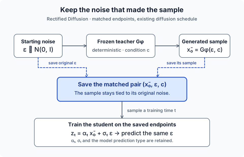
Why Straightness Is Not Required
Suppose an ideal retrained model predicts the same \(\epsilon\) everywhere along one paired path. Its clean-data prediction is then also fixed at \(\tilde{x}_0\). For \(s<t\), a DDIM update gives
Thus one update reaches exactly the same paired path at the next time, even when that path is curved in the original coordinates. The displayed form assumes \(\alpha_t>0\), as in the finite terminal schedule of the noise-prediction model used here. A VP schedule with \(\alpha_t^2+\sigma_t^2=1\) generally traces a curve between the endpoints; setting \(\alpha_t=1-t\) and \(\sigma_t=t\) recovers the straight flow-matching path.
The paper calls this a first-order ODE path: it means the first-order diffusion solver is exact under constant noise prediction, not that other diffusion ODEs involve higher-order derivatives. Exactness is an ideal condition requiring consistent predictions and compatible paths. Finite models, intersecting interpolations, and optimization errors prevent it from being a universal one-step guarantee.
Implementation Overview
This pseudocode describes basic rectification for a text-conditioned, noise-predicting latent diffusion model. The teacher’s final latents, original starting noise, and conditions are stored together.
import copy
import torch

# Stage 1: collect matched endpoints with a frozen teacher.
teacher.eval().requires_grad_(False)
for condition in training_conditions:
    eps = torch.randn(latent_shape, device=device)
    with torch.no_grad():
        x0 = deterministic_teacher_sample(
            teacher, initial_noise=eps, condition=condition,
            steps=teacher_steps, guidance_scale=teacher_cfg,
        )  # return the clean latent, before VAE decoding
    pair_store.add(x0.detach(), eps.detach(), condition)

# Stage 2: initialize from the teacher and keep its parameterization.
student = copy.deepcopy(teacher).train().requires_grad_(True)
optimizer = make_optimizer(student.parameters())
for x0, eps, condition in pair_loader:
    t = sample_training_times(x0.shape[0], device=x0.device)
    a, s = broadcast_schedule(t, x0)  # original alpha_t, sigma_t
    z = a * x0 + s * eps            # saved noise, not fresh noise
    prediction = student(z, t, condition)
    loss = (prediction - eps).square().mean()  # w(t) = 1 here
    optimizer.zero_grad()
    loss.backward()
    optimizer.step()

# Inference uses fresh noise and the retrained model.
student.eval()
with torch.no_grad():
    latent = deterministic_sample(
        student, initial_noise=torch.randn(latent_shape, device=device),
        condition=prompt_embedding, steps=few_steps,
    )
    image = vae.decode(latent / vae_scaling_factor)
Results and Trade-offs
In the paper’s COCO-2017 validation comparison at \(512\times512\) resolution, basic Rectified Diffusion achieves FID 27.26 in one step, versus 47.91 for its rectified-flow baseline. The separate version with subsequent consistency distillation reaches 22.83; that number should not be attributed to paired retraining alone. The teacher still determines the training samples, and producing those pairs has an offline cost. The paper also studies phased rectification, which fits the solver property over shorter time intervals, and consistency distillation for further improvements at very low step counts. Those are additional procedures beyond the basic algorithm above.
References:
- Wang et al. Rectified Diffusion: Straightness Is Not Your Need in Rectified Flow, 2024; ICLR 2025 — Sections 2.1–2.4, Algorithm 4, and Table 1.
- Official implementation: Rectified-Diffusion.
- Liu, Gong, and Liu. Flow Straight and Fast: Learning to Generate and Transfer Data with Rectified Flow, ICLR 2023.
- Esser et al. Scaling Rectified Flow Transformers for High-Resolution Image Synthesis, ICML 2024.
Caching in Diffusion Models
This technique takes advantage of the U-Net architecture used in diffusion models, particularly its skip connections, which transfer intermediate features from the encoder to the decoder.
The core idea:
👉 Store intermediate results from step \(t\) (e.g., decoder features) and reuse them at step \(t-1\) instead of recomputing the entire U-Net.
U-Net Refresher
A U-Net has two main components:
- Encoder (Down Blocks) — progressively downsamples the input to a compact high-level representation.
- Decoder (Up Blocks) — upsamples the features to reconstruct the image.
Each pair of down and up blocks \(D_i, U_i\) connects through:
- a main path: \(D_1 \to D_d \to U_d \to U_1\)
- skip connections: \(D_i \to U_i\)
At each layer, the output combines both paths: \(U_i = \text{Concat}(D_i, U_{i+1})\)
Observation: Feature Reuse Across Timesteps
During denoising, adjacent timesteps produce very similar high-level features: \(U_i^{(t)} \approx U_i^{(t-1)}\)
So instead of recomputing these expensive decoder features every step, we can cache them:
\[F_c^{(t)} \leftarrow U_i^{(t)} \\ U_i^{(t-1)} = \text{Concat}(D_i^{(t-1)}, F_c^{(t)})\]This simple reuse cuts redundant computation and significantly speeds up inference.

Implementation Overview
I was curious more about the implementation details than the idea. You can find the full implementation in the DeepCache repository. First, we need to modify the Stable Diffusion pipeline, specifically the denoising loop, where cached features are passed to the U-Net.
    # predict the noise residual
    noise_pred, prv_features = self.unet(
        latent_model_input,
        t,
        encoder_hidden_states=prompt_embeds,
        cross_attention_kwargs=cross_attention_kwargs,
        replicate_prv_feature=prv_features,
        quick_replicate= cache_interval>1,
        cache_layer_id=cache_layer_id,
        cache_block_id=cache_block_id,
        return_dict=False,
    )
The U-Net model is defined in the unet_2d_condition.py file, where forward method has been modified to support the caching feature.
Note that the caching applied to cross-attention layer only.
if quick_replicate and replicate_prv_feature is not None:
    # Downsampling - nothing change

    # Middle - No middle

    # Upsampling
    sample = replicate_prv_feature
    #down_block_res_samples = down_block_res_samples[:-1]
    if cache_block_id == len(self.down_blocks[cache_layer_id].attentions) :
        cache_block_id = 0
        cache_layer_id += 1
    else:
        cache_block_id += 1

    for i, upsample_block in enumerate(self.up_blocks):

        # Skip the blocks that are not the cache layer # IMPORTANT - This is where speed is gained
        if i < len(self.up_blocks) - 1 - cache_layer_id:
            continue

        if i == len(self.up_blocks) - 1 - cache_layer_id:
            trunc_upsample_block = cache_block_id + 1
        else:
            trunc_upsample_block = len(upsample_block.resnets)

        is_final_block = i == len(self.up_blocks) - 1

        res_samples = down_block_res_samples[-trunc_upsample_block:]
        down_block_res_samples = down_block_res_samples[: -trunc_upsample_block]

        # if we have not reached the final block and need to forward the
        # upsample size, we do it here
        if not is_final_block and forward_upsample_size:
            upsample_size = down_block_res_samples[-1].shape[2:]

        if hasattr(upsample_block, "has_cross_attention") and upsample_block.has_cross_attention:
            #print(sample.shape, [res_sample.shape for res_sample in res_samples])
            sample, _ = upsample_block(
                hidden_states=sample,
                temb=emb,
                res_hidden_states_tuple=res_samples,
                encoder_hidden_states=encoder_hidden_states,
                cross_attention_kwargs=cross_attention_kwargs,
                upsample_size=upsample_size,
                attention_mask=attention_mask,
                encoder_attention_mask=encoder_attention_mask,
                enter_block_number=cache_block_id if i == len(self.up_blocks) - 1 - cache_layer_id else None,
            )
        else:
            sample = upsample_block(
                hidden_states=sample,
                temb=emb,
                res_hidden_states_tuple=res_samples,
                upsample_size=upsample_size,
                scale=lora_scale,
            )

    prv_f = replicate_prv_feature
References:
Vision-Language Models
A rapidly growing branch of generative AI focuses on** Vision-Language Models (VLMs)** — a class of multimodal models that can process and generate information across different input types (modalities), such as text, image, video, and audio. While the input may come from multiple modalities, the output is often text (e.g., in Visual Question Answering, or VQA), but can also be images (e.g., in image captioning or text-to-image generation) or other modalities depending on the task.

Representation Learning in Vision-Language Models
In VLMs, the encoder pathway typically includes separate encoders for each modality, followed by a fusion layer that integrates features from the different modalities. However, as discussed in [2], there are multiple approaches for learning joint multimodal representations that capture cross-modal interactions:
-
Representation Fusion – integrating information from two or more modalities, effectively reducing the number of separate representations.
-
Representation Coordination – exchanging information across modalities to enrich each modality’s context while maintaining the same number of representations.
-
Representation Fission – generating a new, decoupled set of representations (often more than the input count) that captures internal structure such as clusters or latent factors.

Pretraining Vision-Language Models
There are various strategies to pretrain Vision-Language Models. The key idea is to align image and text representations and feed the fused representation into a text decoder for generation tasks. A common architecture consists of three main components:
- Image Encoder – processes raw visual data into a sequence of fixed-length embeddings.
- Multimodal Projector – aligns image and text representations using a dense neural network.
- Text Decoder – generates text output from the fused multimodal representation, usually derived from a pre-trained LLM.
Because the text decoder (or text encoder-decoder) is often initialized from a pretrained LLM, it is typically kept frozen during pretraining. The focus instead is on fine-tuning the multimodal projector, which learns to map the visual features into the same embedding space as the textual features.

Qwen VL

Qwen1-VL consists of:
-
a Vision Transformer (ViT) as the vision encoder (initialized with pre-trained weights from OpenCLIP’s ViT-bigG),
-
a Large Language Model (LLM) serving as both text encoder and decoder (Qwen1 model), and
-
a Position-Aware Vision-Language Adapter (VL-Adapter) bridging the visual and textual spaces. The VL-Adapter is a single-layer cross-attention module initialized randomly. It employs a set of trainable query vectors and uses visual features as keys for cross-attention, compressing the image feature sequence to a fixed length (typically 256). To preserve spatial information, 2D absolute positional encodings are added to the query-key pairs.
Image Input Images are processed through the visual encoder and adapter, yielding fixed-length sequences of image features. To differentiate between image feature input and text feature input, two special tokens (<img> and </img>) are appended to the beginning and end of the image feature sequence respectively, signifying the start and end of image content.
Bounding Box Input and Output Qwen1 VL also supports bounding box reasoning, e.g., for object detection task where the query question can be “Can you find the dog in the image?”. In order to have this capability, the input bounding box coordinates are transformed into a specified string format:
<box>(X-top-left, Y-top-left), (X-bottom-right, Y-bottom-right)</box>
This design allows bounding boxes to be tokenized like text, requiring no extra positional embeddings.
To link textual descriptions with corresponding regions, additional tokens <ref> and </ref> are introduced, e.g.,
"<box>(X-topleft, Y-topleft), (X-bottomright, Y-bottomright)</box><ref>a dog chasing a cat</ref>"
Training Qwen1 VL consists of three stages: two stages of pre-training and a final stage of instruction fine-tuning training.

- Pre-training: The goal of this stage is to joint the visual understanding (through the visual encoder and adapter) with the text understanding from the LLM model. Therefore, in this stage, only the ViT encoder and the adapter are fine-tuned, while the LLM is frozen. The training set is a large-scale, weakly labeled, web-crawled set of image-text pairs. The objective is to predict the text description of the image.
- Multitask Pre-training The goal of this stage is introducing vision-language capabilities to the VLM model (after having a basic visual understanding through pre-training) by introducing high-quality and fine-grained VL annotation data with a larger input resolution and interleaved image-text data. As shown in Table below, the Qwen1 VL was trained on on 7 tasks simultaneously, including image captioning, VQA, OCR, Grounding, etc.
- Supervised Fine-tuning The goal of the last stage is to enhance instruction following and dialogue capabilities, resulting the model can work in Chatbot mode. The multi-modal instruction tuning data primarily comes from caption data or dialogue data generated through LLM self-instruction, which often only addresses single-image dialogue and reasoning and is limited to image content comprehension. To enhance multiple-image comprehension, an additional and manually annotated dataset - which consists of multiple images and set of dialogues - was introduced to train the model. In this stage, we need to optimize the language model and adapter module, while the visual encoder is frozen.

Resources:
- [1] Multimodal machine learning (MMML) Course from CMU https://cmu-mmml.github.io/
- [2] Liang, P. P., Zadeh, A., & Morency, L. P. (2024). Foundations & trends in multimodal machine learning: Principles, challenges, and open questions. ACM Computing Surveys, 56(10), 1-42.
- [3] Vision Language Models Explained https://huggingface.co/blog/vlms
- [4] What are vision language models (VLMs)? by IBM Research https://www.ibm.com/think/topics/vision-language-models
3D Diffusion Models
An image describes how an object looks from one camera. A 3D representation must also describe what happens when we move that camera: which surfaces become visible, what lies behind the object, and how its shape changes the shading. The diffusion machinery remains useful, but we first need to decide what the model denoises.
There are two useful routes:
- Learn a distribution of 3D objects: train diffusion on point clouds or learned 3D representations, then sample a new object with the trained model. Point-E and Shap-E follow this route.
- Use a 2D diffusion model to optimize a 3D object: render the current object, ask a frozen image model for an improvement direction, and update the object through a differentiable renderer. DreamFusion follows this route.
The distinction matters: in the first route, training is shared across future samples; in the second, generating each object requires a new optimization process. These foundational methods illustrate the design choices rather than a ranking of current 3D generators.
Point-E: Diffusion on Colored Point Clouds
Representation and forward process
Point-E (Nichol et al., 2022) represents an object as a tensor \(P_0 \in \mathbb{R}^{N \times 6}\). Each row contains a point’s three coordinates and RGB color, normalized to \([-1,1]\). We can corrupt this tensor using exactly the Gaussian process used for images:
Here \(\bar{\alpha}_t\) is the cumulative signal-retention factor, with clean data at \(t=0\). A transformer predicts the noise in all six channels, conditioned on a reference image \(c\). The simplified noise-prediction objective is
where the Frobenius norm sums over points and channels. Point-E also learns the reverse-process variance; this expression isolates the denoising component.
How does an image guide an unordered set?
The transformer receives point embeddings, a timestep embedding, and 256 image-grid embeddings from a frozen CLIP ViT-L/14. Point tokens have no positional encoding based on their row index: swapping two input points swaps the corresponding predictions. This is permutation equivariance, which preserves the interpretation of the tensor as a set while retaining pointwise noise targets.
The full pipeline first generates a synthetic view using a GLIDE model fine-tuned on 3D renderings. A base point-cloud diffusion model generates 1,024 points conditioned on that image. A second diffusion model keeps these points as conditioning and generates 3,072 additional points, producing 4,096 points in total. The diagram highlights where diffusion acts and why upsampling adds new points instead of replacing the initial set.
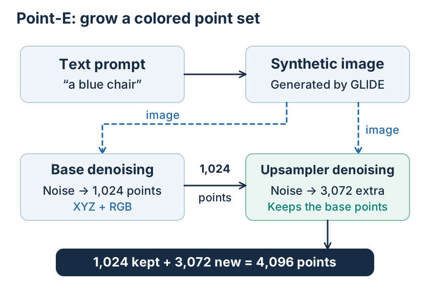
Simplified training and sampling
# P0: normalized XYZRGB points, shape [batch, N, 6].
# schedule.add_noise implements the forward equation above.
t = schedule.sample_timesteps(P0.shape[0], device=P0.device)
eps = torch.randn_like(P0)
Pt = schedule.add_noise(P0, eps, t)
eps_hat = point_model(Pt, t, image_features)
loss = (eps_hat - eps).square().mean()  # Variance loss omitted.
optimizer.zero_grad()
loss.backward()
optimizer.step()

@torch.no_grad()
def generate_points(prompt):
    image = text_to_image(prompt)             # GLIDE in Point-E.
    image_features = frozen_clip_grid(image)
    # Each helper runs a complete reverse diffusion trajectory.
    coarse = sample_point_diffusion(
        base_model, shape=(1, 1024, 6), image=image_features
    )
    extra = sample_point_diffusion(
        upsampler, shape=(1, 3072, 6), image=image_features,
        fixed_points=coarse
    )
    return torch.cat([coarse, extra], dim=1)
These are conceptual helpers, not the package’s exact API. The official notebooks provide runnable sampling examples. A point cloud has no mesh connectivity; Point-E uses a separate model to regress a signed distance field, extracts its zero surface with marching cubes, and transfers colors from nearby points. This conversion can lose thin structures or amplify gaps already present in the points.
Shap-E: Denoising the Parameters of a 3D Function
A point set explicitly lists a finite collection of samples. An implicit representation instead answers a query at a 3D coordinate: what is the density, surface distance, or color here?
Shap-E (Jun and Nichol, 2023) trains an encoder on point clouds and rendered views to produce latents \(z_0=E(\text{asset})\). A learned projection turns these latents into parameters \(\psi\) of an MLP representing the object. The MLP supports both a radiance-field representation and a signed-distance-and-texture representation, so the generated asset can be rendered as a NeRF or extracted as a textured mesh.
After learning this representation, Shap-E trains diffusion on the encoded assets. Its denoiser predicts the clean latent \(\hat z_0\) rather than noise:
Here \(c\) is text or image conditioning. The latents have shape \(1024 \times 1024\), so “latent” does not necessarily mean lower-dimensional than a point cloud. The benefit is a learned representation whose decoded function supports multiple rendering methods.
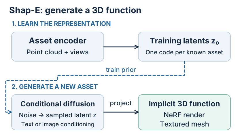
# Conceptual inference; no per-object optimization is required.
z = sample_latent_diffusion(condition, prediction_type="x0")
implicit_parameters = project_latents_to_mlp(z)
image = render_nerf(implicit_parameters, camera)
mesh = extract_textured_mesh(implicit_parameters)
Changing the representation does not solve all conditioning problems. In the paper’s comparison of 300M-parameter models, text-conditional Shap-E improves on Point-E’s CLIP-based metrics, while image-conditional versions reach similar performance and share failure cases. Missing information in the conditioning image and limits of the training data still matter.
DreamFusion: A 2D Diffusion Model as a 3D Learning Signal
Why optimize through rendered views?
DreamFusion (Poole et al., 2022) uses a pretrained text-to-image model without training a diffusion model on 3D data. Let \(\theta\) describe a NeRF-like scene, and let
be its rendered image from camera \(v\) under lighting \(\ell\). DreamFusion’s scene network predicts density and albedo; differentiable volume rendering and shading connect these properties to image pixels. Updating a visible pixel can therefore update the underlying geometry and appearance.
Each iteration samples a camera, renders the scene, and corrupts that rendering:
The frozen image denoiser returns a classifier-free-guided prediction \(\hat\epsilon_\phi(x_t,t,y)\) for prompt \(y\). It never directly predicts a 3D object. The renderer is the bridge between its image-space knowledge and the scene parameters.
Score Distillation Sampling (SDS)
A useful starting point is to make noisy renders agree with the image model’s noisy conditional distribution:
Here \(q_t=\mathcal{N}(a_t x,\sigma_t^2I)\) and \(k(t)\) weights noise levels. Using the diffusion score \(s_\phi=-\hat\epsilon_\phi/\sigma_t\) gives the SDS gradient estimator
The subtracted noise is a zero-mean control variate that reduces variance. The relation between \(w(t)\) and \(k(t)\) also explains why implementations can show different apparent factors of \(a_t\) or \(\sigma_t\): they may absorb them into their weighting convention. DreamFusion uses the final gradient weight \(w(t)=\sigma_t^2\).
👉 The crucial detail is where gradients flow. SDS uses the predicted residual as a fixed image-space gradient and backpropagates it through the renderer. It does not differentiate through the denoiser. Freezing the denoiser’s parameters alone would not enforce this: computing a noise-prediction squared error and backpropagating through its input would still introduce the denoiser Jacobian, giving a different update.
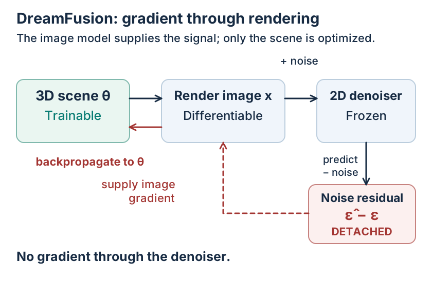
Implementation of the SDS update
# PyTorch-style pseudocode. The optimizer contains scene parameters only.
# The denoiser is an epsilon predictor; images use its expected scaling.
for step in range(num_optimization_steps):
    camera, light = sample_camera_and_light()
    image = render(scene, camera, light)  # Keep this computation graph!
    t = sample_uniform_time(0.02, 0.98)
    a_t, sigma_t = diffusion_coefficients(t)
    eps = torch.randn_like(image)

    with torch.no_grad():
        noisy_image = a_t * image.detach() + sigma_t * eps
        eps_u = denoiser(noisy_image, t, null_condition)
        eps_c = denoiser(noisy_image, t, view_condition(prompt, camera))
        eps_guided = eps_u + guidance_scale * (eps_c - eps_u)
        image_gradient = sigma_t**2 * (eps_guided - eps)

    # A surrogate scalar whose image gradient is exactly the SDS signal.
    # Sum pixels/channels, average the sampled views in the batch.
    loss_sds = (image_gradient.detach() * image).flatten(1).sum(1).mean()
    loss = loss_sds + geometry_regularization(scene, camera)
    optimizer.zero_grad()
    loss.backward()
    optimizer.step()
The surrogate’s numerical value is not a denoising error or an estimate of the KL itself; its purpose is to produce the desired gradient. Random cameras couple observations through the same scene. DreamFusion also uses randomized lighting, textureless renders, view-dependent text conditioning, and opacity/orientation penalties to discourage flat, painted solutions.
Evidence and limitations
DreamFusion’s original implementation uses Imagen’s 64 × 64 base model, with 15,000 optimization iterations taking about 1.5 hours on four TPUv4 chips. On 153 object-centric COCO prompts, it reports CLIP ViT-L/14 R-Precision of 79.7% for color renders and 58.5% for textureless renders. The latter tests whether geometry remains recognizable without texture, but neither metric certifies geometric correctness.
Point-E reports 1–2 minutes on one GPU, with lower sample quality in its original evaluation; hardware and rendering protocols differ, so these are reported operating points rather than a controlled speed ratio. Shap-E improves representation flexibility but still needs a learned 3D dataset. DreamFusion avoids that requirement for its optimization procedure, yet remains vulnerable to ambiguous views, flat geometry, oversmoothing, saturated colors, and limited diversity. A plausible image from several views is useful evidence for a 3D object, but it is not a unique specification of its shape.
References:
- [1] Nichol et al. Point-E: A System for Generating 3D Point Clouds from Complex Prompts, 2022. Official implementation.
- [2] Jun and Nichol. Shap-E: Generating Conditional 3D Implicit Functions, 2023. Official implementation.
- [3] Poole et al. DreamFusion: Text-to-3D using 2D Diffusion, ICLR 2023. Project and generated examples.
Diffusion Language Models
An autoregressive language model generates a sequence \(x_0=(x_0^1,\ldots,x_0^L)\) by predicting the next token from its prefix:
Diffusion language models instead learn to recover text from corrupted text or corrupted text representations. At generation time, they repeatedly denoise an entire sequence, allowing predictions to use the visible context on both sides of a missing token. The main design question is what should noise mean for text? Adding Gaussian noise to an integer token ID would introduce an arbitrary geometry: neighboring IDs need not represent similar words.
Continuous Embeddings or Discrete Tokens?
There are two useful starting points:
| Approach | What is corrupted? | What does the model predict? | How does generation finish? |
|---|---|---|---|
| Continuous diffusion, e.g., Diffusion-LM | A sequence of real-valued word embeddings | Clean embeddings or a related denoising target | Convert denoised vectors into vocabulary tokens |
| Discrete diffusion, e.g., D3PM and MDLM | Tokens through categorical transitions, including replacement by a mask | Probabilities over clean vocabulary tokens | Sample tokens directly from the reverse process |
Diffusion-LM (Li et al., 2022) learns an embedding function \(E\) and performs Gaussian diffusion over its outputs. Writing \(z_0\approx E(x_0)\in\mathbb{R}^{L\times d}\), the familiar forward marginal becomes
Here \(d\) is the embedding dimension. The approximation in \(z_0\approx E(x_0)\) omits the paper’s small initial Gaussian perturbation around the learned embeddings. A Transformer denoises these continuous variables, while a learned token decoder rounds the final vectors into text. The embeddings and denoiser are trained jointly; predicting \(z_0\) and clamping intermediate predictions toward nearby word embeddings help reduce rounding errors.
The continuous intermediate states also provide a place to apply classifier guidance: gradients of a control model can steer the latent sequence toward a requested attribute, such as a syntactic structure. The paper’s figure shows this connection between the diffusion trajectory and the control signal.

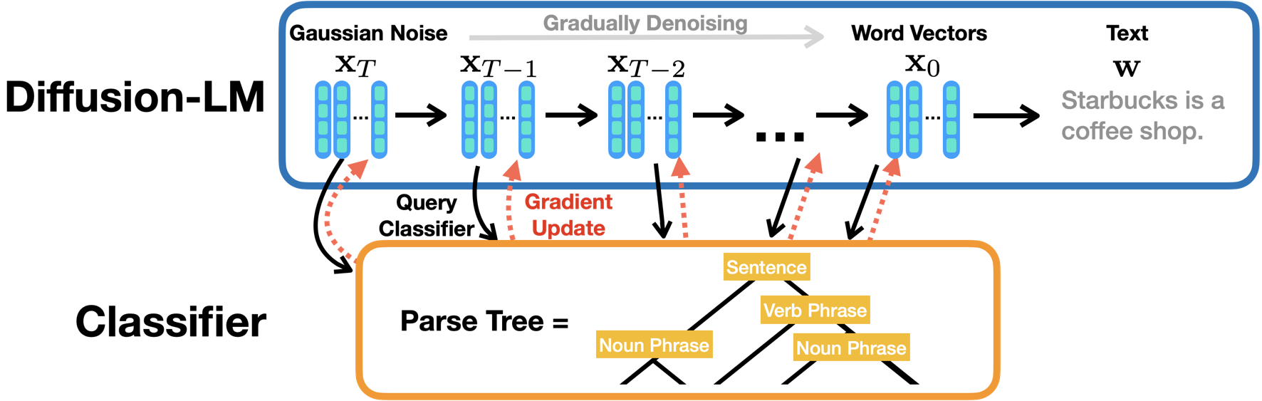
D3PM (Austin et al., 2021) takes the other route: it defines a transition matrix whose entries give the probability of changing one token into another. Corruption can be uniform, structured by embedding similarity, or directed into an absorbing mask state. Absorbing-state diffusion gives an especially simple language model, which we derive next using MDLM (Sahoo et al., 2024).
Forward Process: Gradually Mask the Sequence
Let \(m\) denote a special [MASK] token that never appears in clean text. Use continuous time \(t\in[0,1]\), where \(t=0\) is clean text and \(t=1\) is fully masked. Define \(\alpha_t\) as the probability that a token remains visible, with \(\alpha_0=1\) and \(\alpha_1=0\). For each position \(i\),
where \(\delta_a\) is a point mass on token \(a\). Tokens are masked independently conditional on the same sampled time. Once masked along a forward trajectory, a token stays masked. For the simple schedule \(\alpha_t=1-t\), each position is masked with probability \(t\).
👉 The denoising problem changes with the noise level: a lightly masked sentence mostly asks for local reconstruction; an almost fully masked sentence requires the model to construct much more of the sentence from its learned language distribution. Training must cover both regimes.
The MDLM figure connects this variable masking process to its weighted reconstruction objective. The benchmark panel is historical evidence from that paper, with diffusion perplexities evaluated through likelihood bounds.

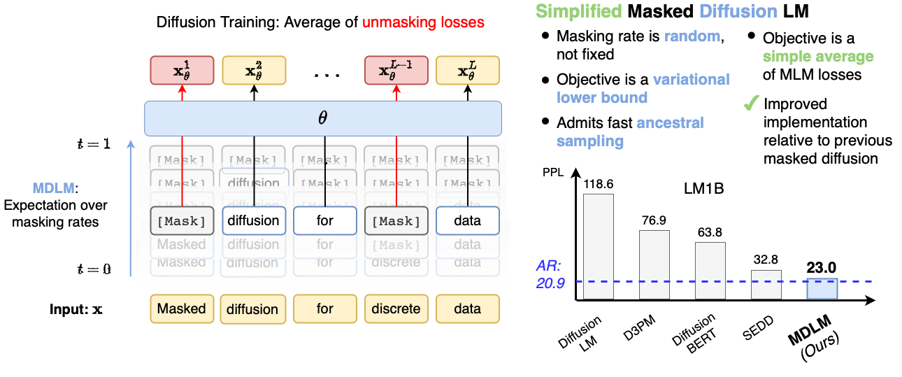
Reverse Process: Decide When and What to Reveal
Consider a reverse step from \(t\) to \(s<t\). If \(x_t^i\neq m\), its original identity is already known, so the reverse step simply copies it. If \(x_t^i=m\), there are two possibilities: it was already masked at \(s\), or it became masked between \(s\) and \(t\). Therefore,
The denominator is the probability that the position is masked at \(t\). The second numerator is the probability mass that was still visible at \(s\) but has disappeared by \(t\). These two probabilities sum to one.
During generation, \(x_0\) is unknown. A bidirectional Transformer predicts a clean-token distribution \(\pi_\theta^i(v\mid x_t,t)\) over ordinary vocabulary tokens \(v\neq m\). Substituting this prediction into the posterior gives
MDLM calls its construction SUBS, for substitution: exclude [MASK] from clean-token predictions, and carry over already visible tokens. With \(\alpha_t=1-t\), a masked position stays masked with probability \(s/t\) and is revealed with probability \((t-s)/t\).
Two different decisions are involved: the schedule determines when a position is revealed; the network determines what token appears there. The model uses the whole visible sequence when predicting each position, even though the usual finite-step reverse kernel samples positions independently conditional on that sequence. Taking large reverse steps therefore approximates dependencies among tokens that become visible simultaneously.
Training Objective: Weighted Masked Cross-Entropy
The same reverse probabilities explain the loss. For a masked position, the true and learned reverse kernels assign identical probability to staying masked. Their KL divergence reduces to the reveal probability multiplied by the clean token’s negative log-probability:
Visible positions contribute zero. Summing over positions and steps, then taking the continuous-time limit, yields the MDLM negative evidence lower bound:
Here \(t\sim\mathcal{U}(0,1)\) and \(\alpha'_t=d\alpha_t/dt<0\). With the clean and fully masked endpoints and the SUBS construction, the endpoint reconstruction and prior terms vanish. For \(\alpha_t=1-t\), the weight simplifies to \(1/t\). This is a mixture of masked language modeling losses across noise levels, tied to a generative likelihood bound; using a fixed masking ratio alone does not supply this construction.
For conditional generation, keep the prompt visible and corrupt only the response. The network receives both the prompt and the partially masked response, while the loss covers masked response positions.
Implementation: Training and Ancestral Sampling
The following is educational PyTorch pseudocode for the linear schedule. model(tokens, t) returns vocabulary logits of shape [batch, length, vocabulary] using bidirectional attention. Clean inputs contain no [MASK] tokens. train_positions marks valid positions to corrupt and supervise: all text positions for pretraining, or response positions for instruction tuning. Padding must also be excluded from attention by the model wrapper.
import torch
import torch.nn.functional as F


def masked_diffusion_loss(model, clean, train_positions, mask_id):
    batch_size = clean.shape[0]
    # A small endpoint cutoff avoids division by zero in finite precision.
    eps = 1e-5
    t = eps + (1.0 - eps) * torch.rand(batch_size, device=clean.device)
    masked = (torch.rand(clean.shape, device=clean.device) < t[:, None])
    masked = masked & train_positions
    noisy = torch.where(masked, mask_id, clean)

    logits = model(noisy, t).float()
    logits = logits.clone()
    logits[..., mask_id] = -torch.inf  # Clean data cannot be a mask.
    nll = F.cross_entropy(logits.transpose(1, 2), clean, reduction="none")

    weighted = torch.where(masked, nll, 0.0) / t[:, None]
    # Normalize by eligible length, not the realized number of masks.
    lengths = train_positions.sum(dim=1).clamp_min(1)
    return (weighted.sum(dim=1) / lengths).mean()


# clean and train_positions come from the data loader.
optimizer.zero_grad()
loss = masked_diffusion_loss(model, clean, train_positions, mask_id)
loss.backward()
optimizer.step()
This code averages the sequence objective per eligible token and omits the tiny interval \(t<\epsilon\). It samples one corrupted sequence per example; training does not run the entire reverse chain. Dividing by the realized mask count instead of the eligible sequence length would change the estimator, particularly for examples with very few masks.
For sampling, start with a fixed prompt and an all-mask response. The code below samples the specified factorized reverse kernel, using the exact reveal probability for each step. It remains a finite-step approximation to the continuous-time generative process.
@torch.no_grad()
def sample_masked_diffusion(model, prompt, response_length, steps, mask_id):
    model.eval()
    batch_size, prompt_length = prompt.shape
    assert steps > 0 and response_length > 0
    assert not prompt.eq(mask_id).any()
    response = torch.full(
        (batch_size, response_length), mask_id,
        dtype=prompt.dtype, device=prompt.device,
    )
    tokens = torch.cat([prompt, response], dim=1)

    for k in range(steps, 0, -1):
        t = torch.full((batch_size,), k / steps, device=tokens.device)
        s = (k - 1) / steps
        masked = tokens.eq(mask_id)
        logits = model(tokens, t).float()
        logits[..., mask_id] = -torch.inf
        candidates = torch.distributions.Categorical(logits=logits).sample()

        # (t - s) / t = 1 / k: reveal each remaining mask independently.
        reveal_probability = (t - s) / t
        reveal = torch.rand(tokens.shape, device=tokens.device)
        reveal = masked & (reveal < reveal_probability[:, None])
        tokens = torch.where(reveal, candidates, tokens)

    return tokens[:, prompt_length:]  # At the final step every mask is revealed.
Already revealed tokens and the prompt are preserved. This absorbing-mask sampler cannot revise a committed token; repeated denoising does not automatically imply unrestricted editing.
From MDLM to LLaDA: Evidence and Trade-offs
MDLM’s LM1B experiment compares 110M-parameter models trained for 327B tokens: its reported perplexity upper bound is 23.00, versus 20.86 exact perplexity for the retrained autoregressive Transformer. This is evidence that a simple masking process can narrow the language-modeling gap. It is not evidence that the diffusion model has lower perplexity; the diffusion result is a bound. (Sahoo et al., 2024, Table 1)
LLaDA scales masked diffusion to 8B parameters, pretraining on 2.3 trillion tokens and instruction tuning on 4.5 million prompt-response pairs. Its Transformer uses bidirectional attention and a time-independent mask predictor. Prompt tokens remain unmasked during instruction tuning. These results show that next-token factorization is not required for the demonstrated language and instruction-following capabilities. The paper’s matched-data autoregressive comparisons cover smaller compute budgets; comparisons with external 8B models also involve different training data. (Nie et al., 2025)
LLaDA also explores low-confidence remasking: predict candidates at masked positions, keep a scheduled number of confident predictions, and leave the others masked. A further option fills blocks from left to right while denoising within each block. These are useful decoding strategies, but confidence-based selection changes the random reveal kernel derived above. It should not be presented as exact ancestral sampling. (LLaDA, Section 2.4)
The remaining practical trade-offs are:
- Parallel predictions still require repeated computation. An autoregressive decoder reuses cached keys and values for its unchanged prefix. Bidirectional denoising changes the context seen by earlier positions, so ordinary autoregressive KV caching does not directly apply. Fewer decoding rounds alone do not establish a wall-clock speedup.
- Generation length needs a policy. The example allocates a fixed response length. Variable-length output requires an end-of-sequence convention, a length choice, or blockwise extension. MDLM explicitly develops semi-autoregressive generation for this purpose.
- Speed, dependence, and quality interact. Revealing many tokens in one pass reduces network calls but commits more tokens without conditioning on each other’s sampled identities. Smaller steps permit more conditioning on newly revealed context, at higher cost. Quality and latency must be measured together for the chosen sampler and hardware. (MDLM, Sections 4 and 5)
References:
- [1] Austin et al. Structured Denoising Diffusion Models in Discrete State-Spaces, NeurIPS 2021.
- [2] Li et al. Diffusion-LM Improves Controllable Text Generation, NeurIPS 2022. Official implementation.
- [3] Sahoo et al. Simple and Effective Masked Diffusion Language Models, NeurIPS 2024. Official implementation.
- [4] Nie et al. Large Language Diffusion Models, 2025. Official implementation.
Enjoy Reading This Article?
Here are some more articles you might like to read next: