Karpathy Series - Building Micrograd
- Lecture overview and objectives
- Micrograd purpose and definition of autograd
- Illustrative scalar computation graph and forward/backward usage
- Meaning of computed gradients for inputs
- Neural networks as mathematical expressions and scalar engine tradeoffs
- Micrograd repository structure and minimalism
- Defining a scalar function and visualizing it
- Numerical approximation of derivatives via finite differences
- Partial derivatives and sensitivity for multi-input functions
- Implementing the Value class and primitive operators
- Visualizing computation graphs with graphviz and labeling nodes
- Introducing .grad and initializing backprop base case
- Manual backpropagation for product nodes and local derivatives
- Applying the chain rule to addition nodes and routing gradients
- Recursing chain rule to compute leaf gradients and numeric verification
- Using gradient information to perform a parameter update
- Mathematical model of a neuron and activation function choice
- Implementing tanh as a Value operation and its backward rule
- Automating local backward logic by storing closures in nodes
- Topological sorting and implementing Value.backward
- Gradient accumulation bug on reused variables and the accumulation fix
- Convenience wrappers for numeric constants and right-side operations
- Adding exp/power, division, subtraction primitives and equivalence of decomposed tanh
- Neural modules: neuron, layer, and MLP abstractions matching common APIs
- Dataset construction, loss definition (MSE), and computing gradients for training
- Parameter update loop, learning rate selection, and iterative optimization
- Zeroing gradients across iterations and consequences of forgetting to zero
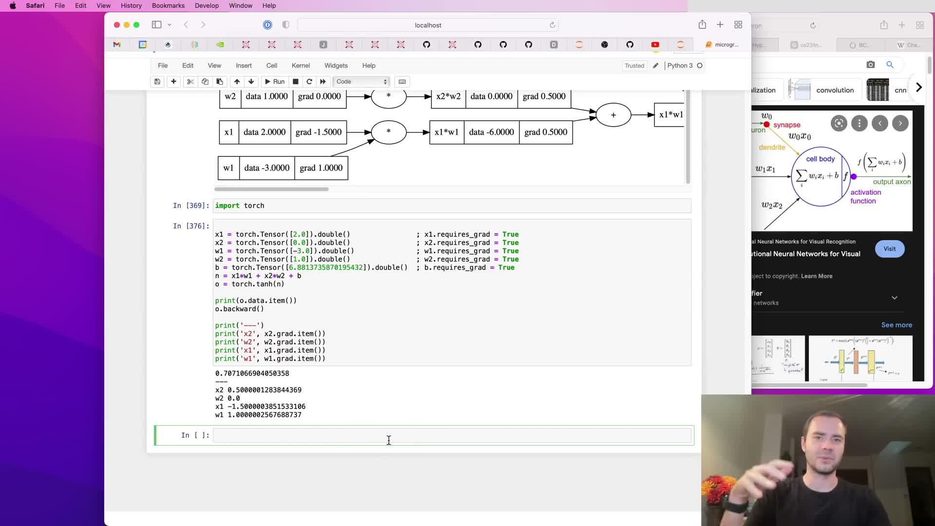
- Comparison with PyTorch implementation details and registering custom ops
- Summary of principles: expressions, loss, backprop, and gradient descent
Lecture overview and objectives
The lecture motivates showing neural network training under the hood by building a minimal automatic-differentiation engine called micrograd and implementing a tiny network end-to-end.
The exercise is framed as starting from an empty Jupyter notebook and proceeding step-by-step to define:
-
data structures for values and graph connectivity
-
forward evaluation to compute numeric outputs
-
backward propagation to compute gradients
- a simple training loop to update parameters
Intended outcome:
- both conceptual and practical understanding of backpropagation, autograd, and how simple operations compose into trainable networks
- emphasis on pedagogical clarity over production performance so every mechanical detail is visible and explicit
This walkthrough lets readers see how the pieces fit before scaling to larger frameworks or vectorized implementations.
Micrograd purpose and definition of autograd
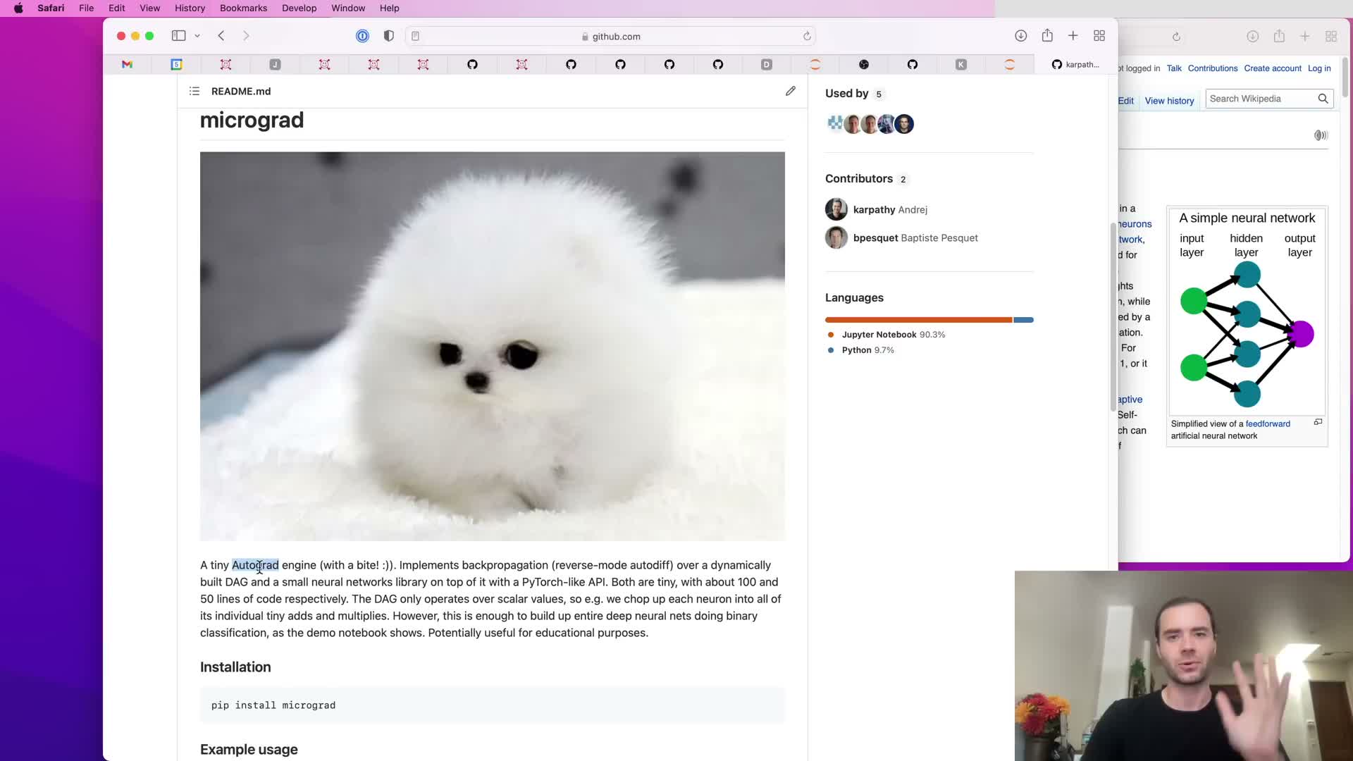
Micrograd is presented as a compact autograd engine — where autograd means automatic computation of gradients — that implements backpropagation to compute gradients of a scalar loss with respect to internal variables or weights.
Key points:
-
Backpropagation efficiently computes derivatives via the chain rule.
- Those derivatives enable iterative optimization of parameters to minimize a loss function.
- Conceptually, micrograd is the mathematical core analogous to the gradient machinery inside larger libraries (e.g., PyTorch, JAX).
- Scope is intentionally limited: demonstrate how arbitrary mathematical expressions can be instrumented to compute gradients so neural-network training becomes straightforward.
Illustrative scalar computation graph and forward/backward usage
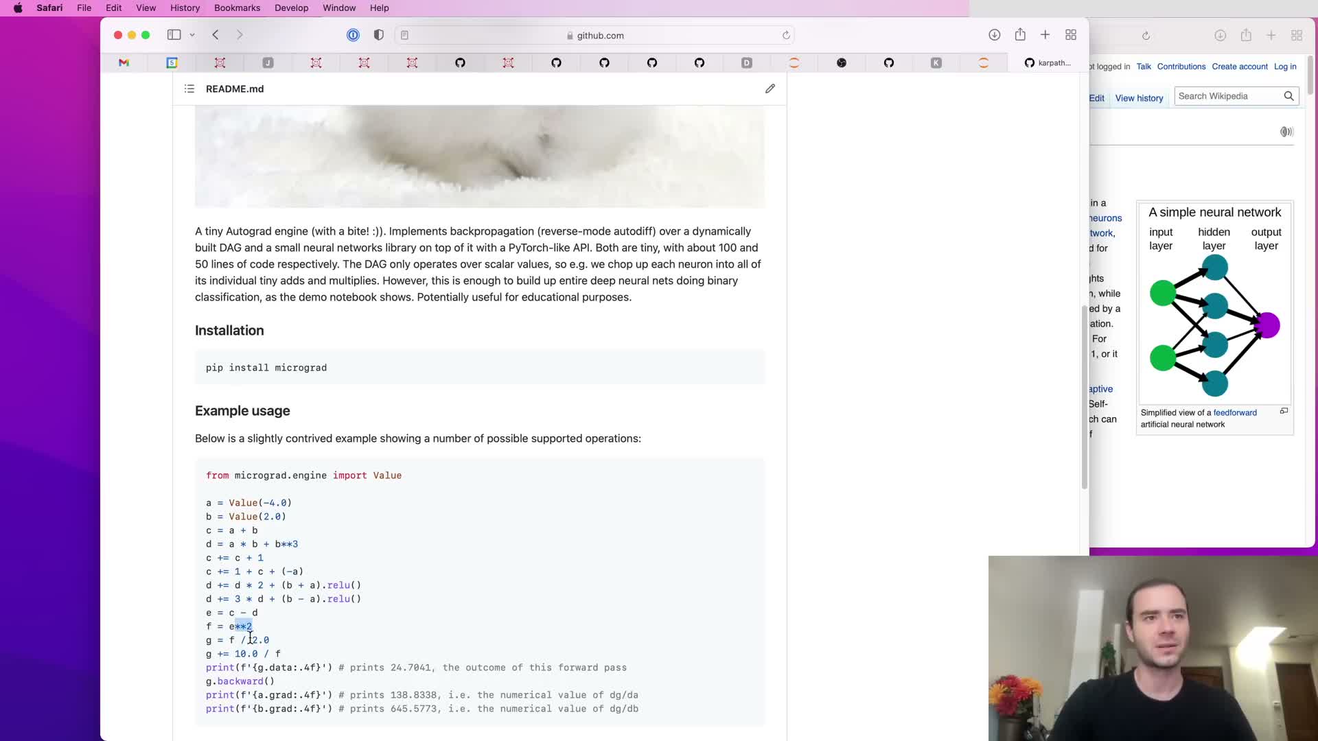
A simple example builds scalar inputs wrapped in a Value object and composes arithmetic operations to form a computation graph.
Flow:
- Create scalar inputs as Value instances.
- Combine them with operations (add, mul, pow, neg, etc.) to form an expression graph.
- The forward pass reads numeric outputs from a data attribute on the resulting Value.
- Calling .backward() on the final output triggers reverse-mode differentiation and populates .grad fields on every node.
Implementation detail:
- Each operation records pointers to operand Value instances and an operation label, building a directed acyclic graph (DAG).
Takeaway: arbitrary mathematical expressions — not just neural layers — are valid targets for automatic differentiation.
Meaning of computed gradients for inputs
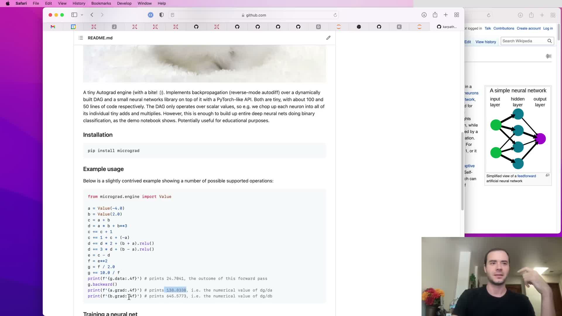
Computed gradients are interpreted as sensitivities: they quantify how a small change in an input affects the output.
Notes:
- The numerical value of a.grad or b.grad is the instantaneous slope ∂output/∂input at the current evaluation point.
- A positive gradient means increasing the input increases the output; a negative gradient means the opposite.
- Gradients provide a local linear approximation used by optimizers to decide how to nudge parameters.
In short: gradients are the fundamental signal exploited by gradient-based optimization methods.
Neural networks as mathematical expressions and scalar engine tradeoffs
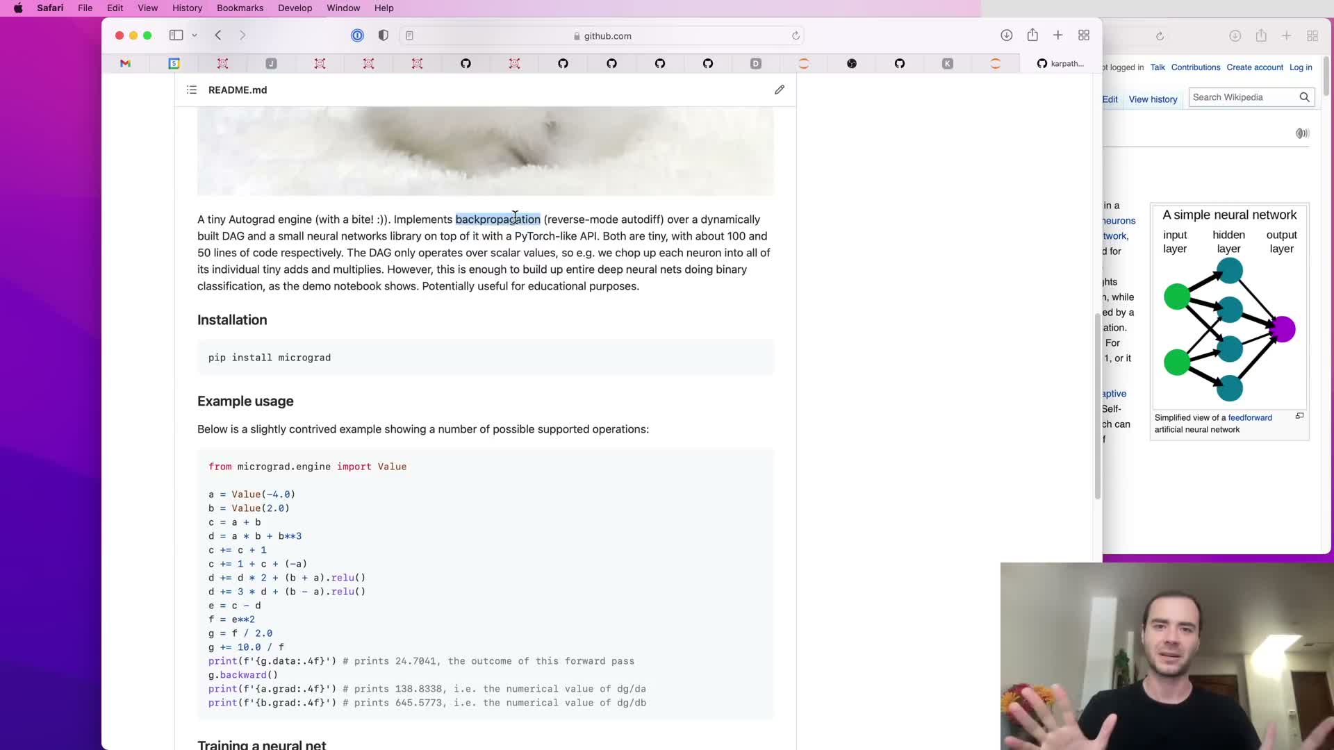
Neural networks are just particular classes of mathematical expressions that map data and weights to predictions and losses.
Consequences:
- A general-purpose autograd engine that handles arbitrary expressions therefore subsumes the needs of neural-network training.
-
Micrograd intentionally operates at the scalar Value level for pedagogical simplicity, making the implementation tiny and explicit but inefficient for large models.
- Production frameworks group scalars into tensors and use vectorized operations to exploit parallel hardware — efficiency changes, but the core calculus does not.
This section clarifies the distinction between pedagogical minimalism and production efficiency while emphasizing unchanged mathematical principles.
Micrograd repository structure and minimalism
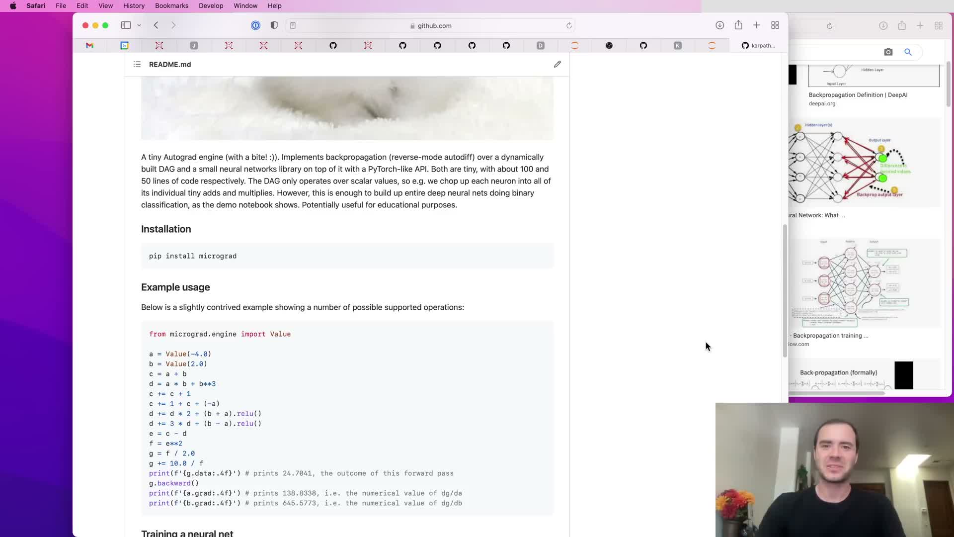
Micrograd is an intentionally tiny codebase with two main files:
-
engine.py — the autograd engine implementing the core Value data structure and backward mechanics (roughly a hundred lines of Python).
-
nn.py — a small neural-network library built on top of the engine with simple abstractions for neurons, layers, and multilayer perceptrons.
Goals of this layout:
- Showcase that essential ideas behind neural training are compact and comprehensible.
- Highlight that larger libraries primarily add efficiency, convenience, and device support.
This frames upcoming implementation tasks and motivates understanding each piece before scaling up.
Defining a scalar function and visualizing it
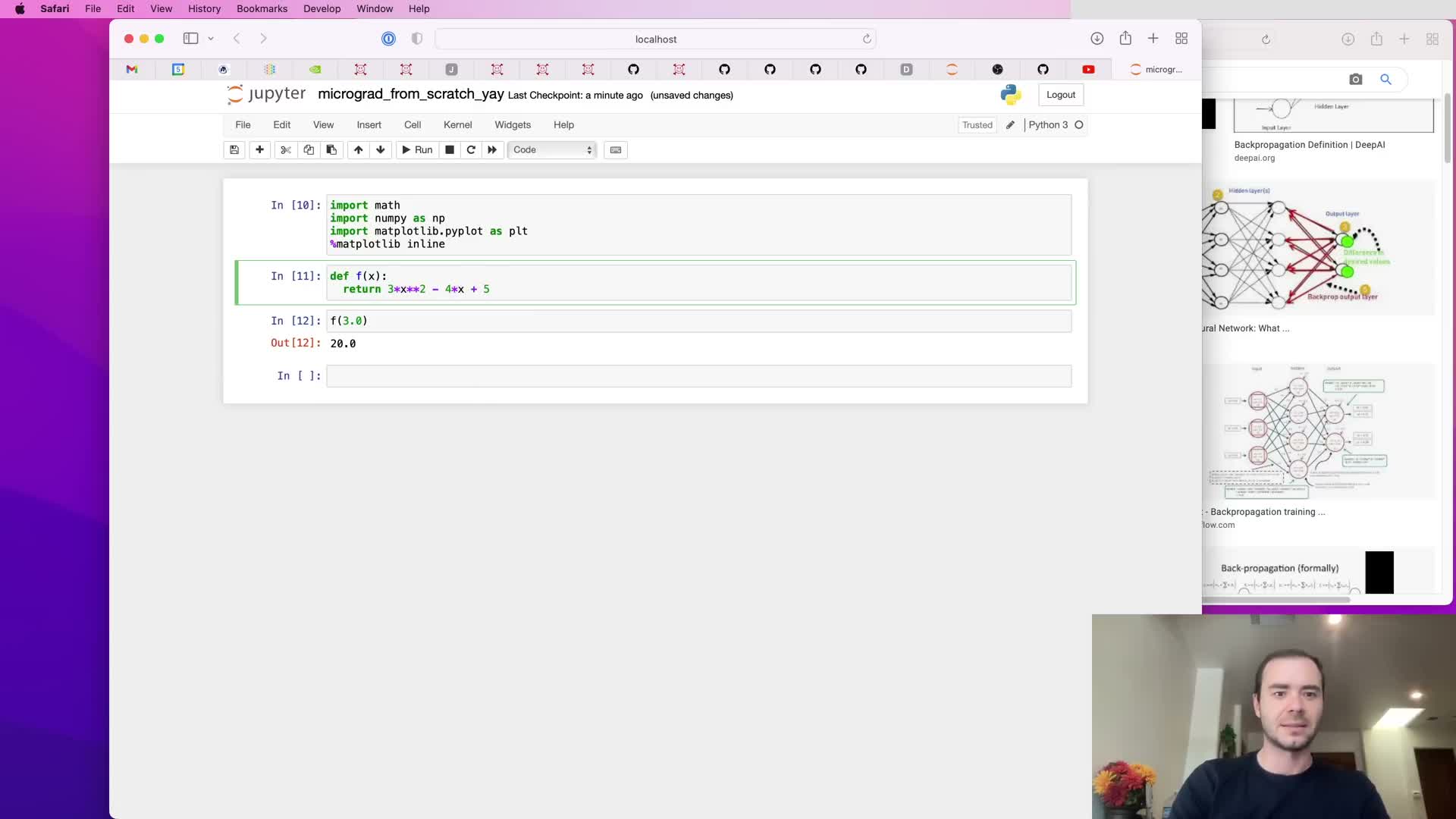
A scalar test function (e.g., a quadratic) is defined to build intuition about function shape and derivatives.
Practice:
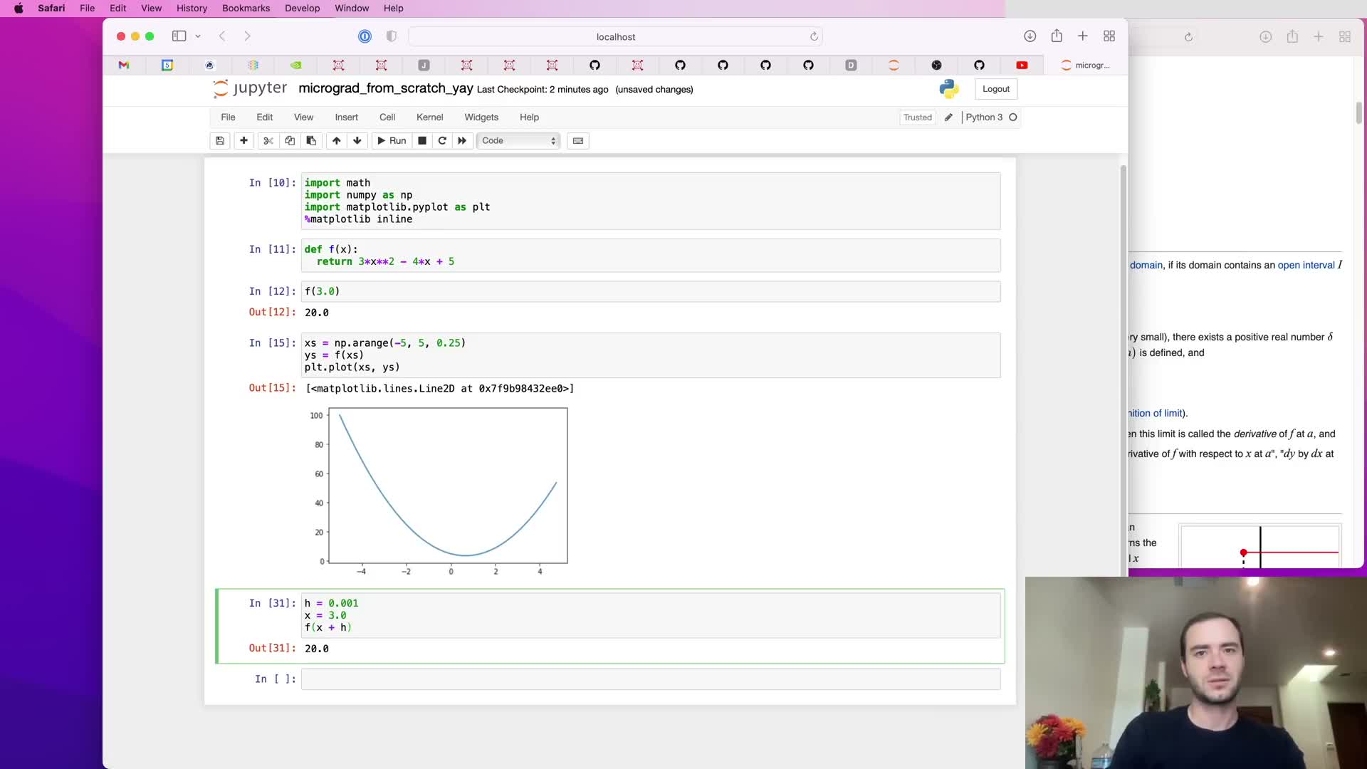
- Plot f(x) over a range to visualize curvature and critical points.
- Use concrete evaluations (e.g., f(3.0)=20) to ground later differentiation examples.
Visual inspection helps reason about:
- Sign and magnitude of derivatives at different x values (positive slope on the right, negative on the left, zero slope at the minimum).
This simple scalar example seeds the transition to numerical and automatic differentiation.
Numerical approximation of derivatives via finite differences
The derivative is introduced formally as the limit of (f(x+h) - f(x)) / h as h → 0, and practical finite-difference approximation uses small but finite h (e.g., 1e-3).
Practical notes:
- Floating-point precision limits the smallest useful h — too small h can produce noisy estimates.
- For simple polynomials, finite differences reproduce analytic results (e.g., analytic f’(3) for 3x^2 - 4x + 5).
- Finite differences serve both as a diagnostic and as an intuitive bridge to automatic differentiation, which computes exact derivatives up to floating-point error without symbolic manipulation.
Emphasize the rise-over-run interpretation and numerical-stability considerations when using finite differences.
Partial derivatives and sensitivity for multi-input functions
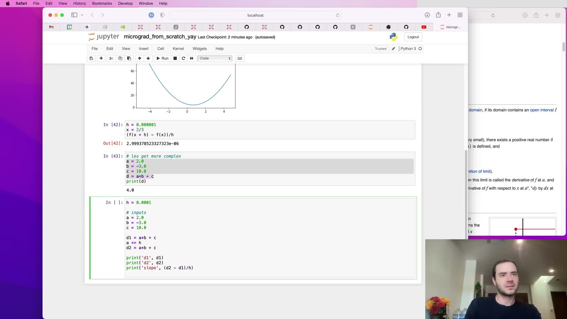
Partial derivatives are extended to functions of multiple scalar inputs via finite-difference experiments.
Method:
- Perturb one input at a time by h and compute (f(…, a+h, …) - f(…, a, …)) / h to estimate ∂f/∂a.
- Repeat for each input to obtain ∂d/∂a, ∂d/∂b, ∂d/∂c.
Illustration:
- For d(a,b,c) = a*b + c, perturbing a yields derivative equal to b, matching analytic expectation.
Takeaway: each partial derivative measures local sensitivity holding other inputs fixed, and these local sensitivities compose via the chain rule in larger graphs — the intuition needed for backpropagation across many inputs.
Implementing the Value class and primitive operators
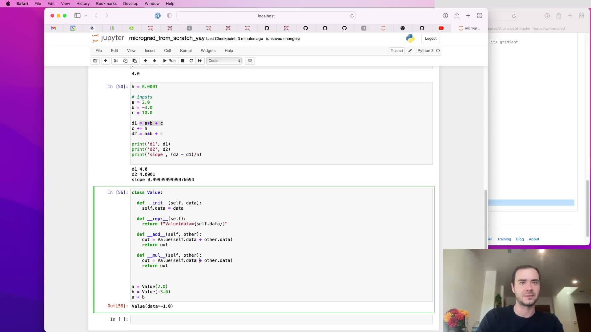
Introduce the Value class as a container for a scalar plus bookkeeping fields required for autograd:
Core fields:
-
data — numeric scalar value.
-
prev / children — references to operand Value nodes (graph edges).
-
op — operation label (e.g., ‘+’, ‘*’, ‘tanh’).
-
grad — gradient initialized to zero.
Operator overloading:
- Implement __add__, __mul__, etc., to produce new Value instances whose data is computed from operands and that record parents and operation type.
Result:
- An explicit computation graph of Value nodes where leaves are inputs/parameters and internal nodes are intermediate computations, enabling traversal for gradient propagation.
Implementation choices include convenience wrappers for readable string formatting and using tuple/set representations for children to balance readability and efficiency.
Visualizing computation graphs with graphviz and labeling nodes
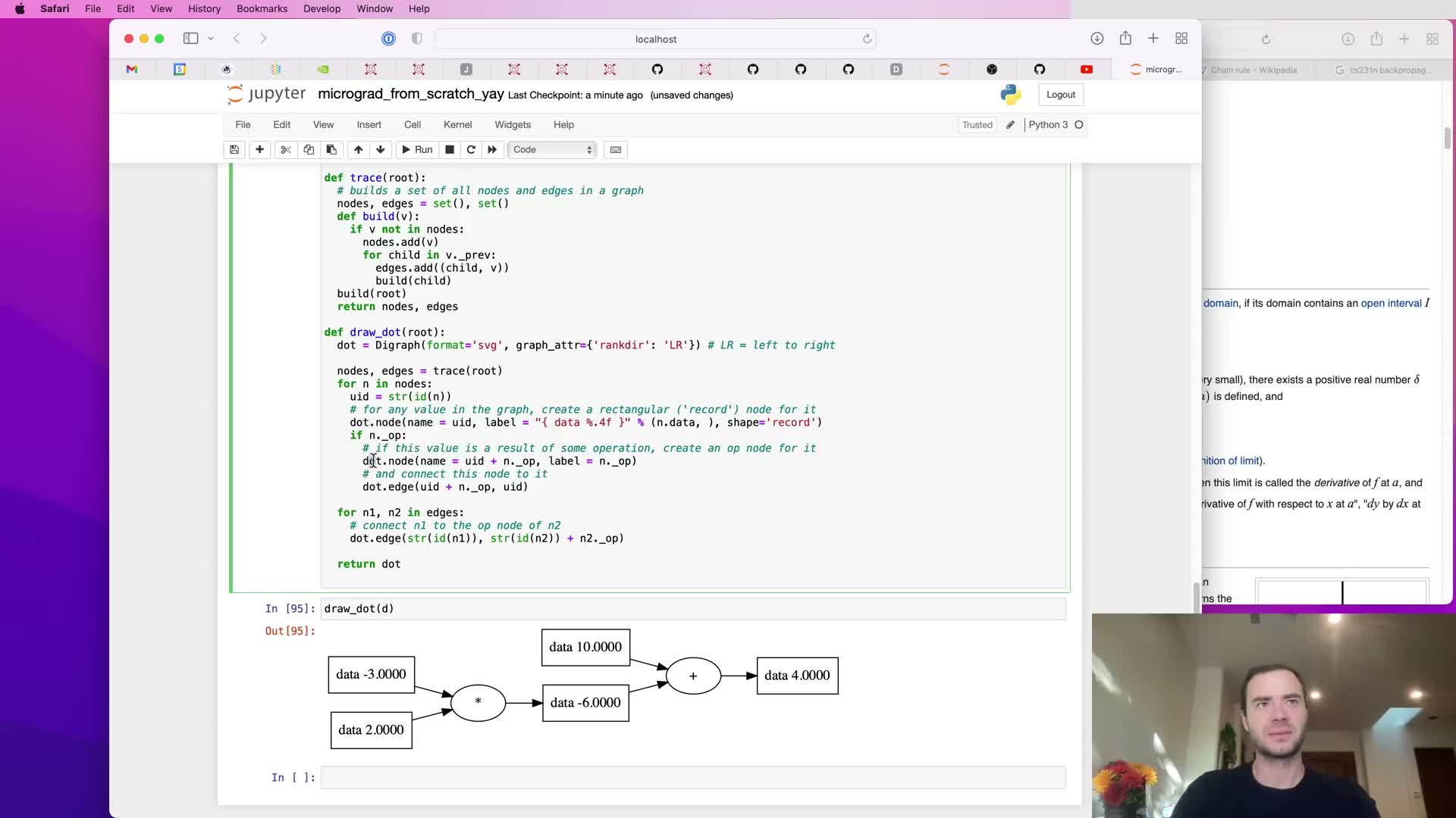
A drawdot routine is added to traverse the Value computation graph and emit a Graphviz representation for visualization.
What it renders:
- Nodes for Value containers and fake operator nodes for readability.
- Labeled edges tracing parent-child relationships so each Value maps back to source expressions.
Benefits:
- Makes the forward computational structure visible.
- Aids reasoning about forward and backward passes and helps verify that .prev and .op fields were set correctly.
This visualization is a practical debugging and pedagogical tool for understanding how expressions expand into a computation DAG.
Introducing .grad and initializing backprop base case
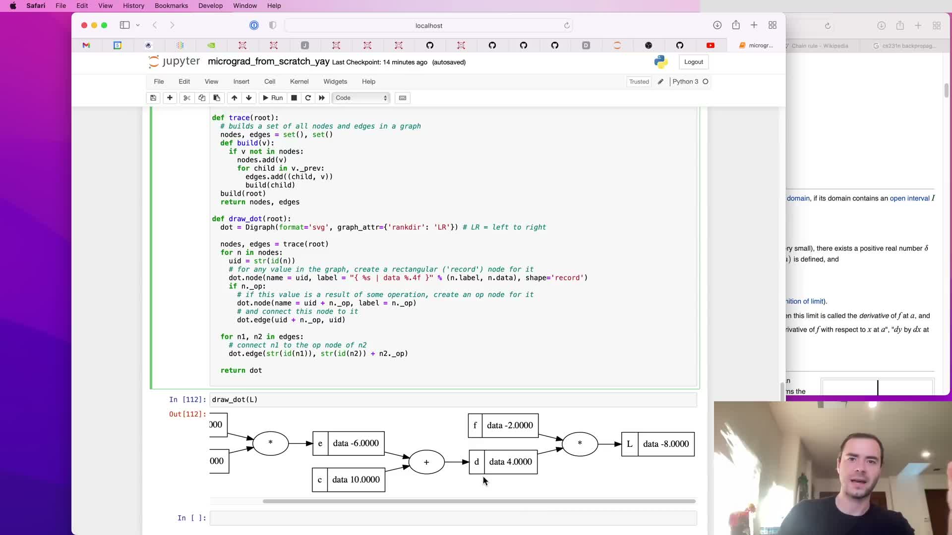
Each Value instance has a .grad attribute representing d(output)/d(node) at the current evaluation; it is initialized to zero to indicate no influence before backpropagation.
Seeding the backward pass:
- The derivative of the output with respect to itself is one, so the final output node’s .grad is set to 1.0 to start accumulation.
Purpose:
- Explicit .grad storage prepares nodes for local backward updates and makes gradient-accumulation semantics clear: gradients measure sensitivity at the current evaluation point.
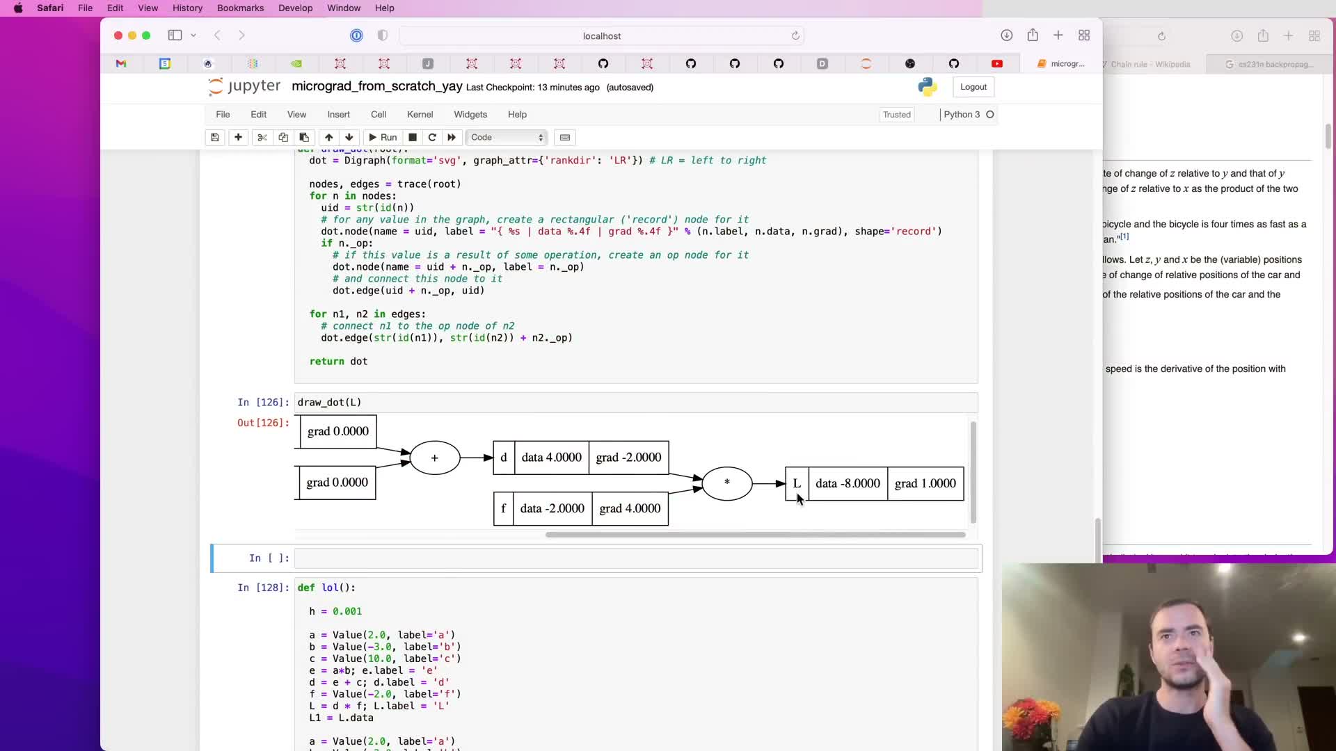
Manual backpropagation for product nodes and local derivatives
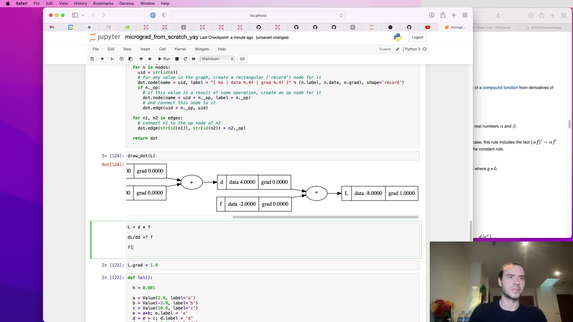
Backpropagation through a multiplication node is illustrated using local derivatives and upstream gradient chaining.
Example:
- For z = x * y, local derivatives are ∂z/∂x = y and ∂z/∂y = x.
- The incoming gradient at z is multiplied by these local factors to propagate to x.grad and y.grad.
Validation:
- The segment shows computing dl/dd and dl/df for a composed example and confirms results algebraically and with finite differences.
Takeaway: each node only needs its local derivative formulas and current operand values to route gradients backward via the chain rule — reinforcing the modularity of autograd where primitive operations supply simple routing rules.
Applying the chain rule to addition nodes and routing gradients
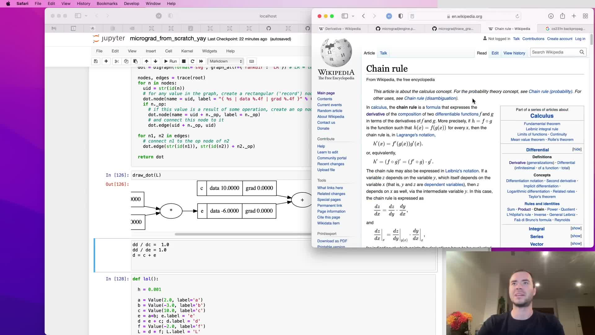
The chain rule is presented for composition and applied to addition nodes to show gradient routing through sums.
Principle:
- For composition z(y(x)), dz/dx = dz/dy * dy/dx.
Addition example:
- For d = c + e, local derivatives ∂d/∂c and ∂d/∂e are both 1.0, so the incoming gradient is copied to both children.
Implications:
- Sum nodes act as distributors of gradient flow.
- Distinguish local derivatives (simple, per-node) from the global gradient accumulated through the graph.
This mechanism is used to compute dl/dc and dl/de by multiplying dl/dd by local derivatives (ones) and assigning to c.grad and e.grad.
Recursing chain rule to compute leaf gradients and numeric verification
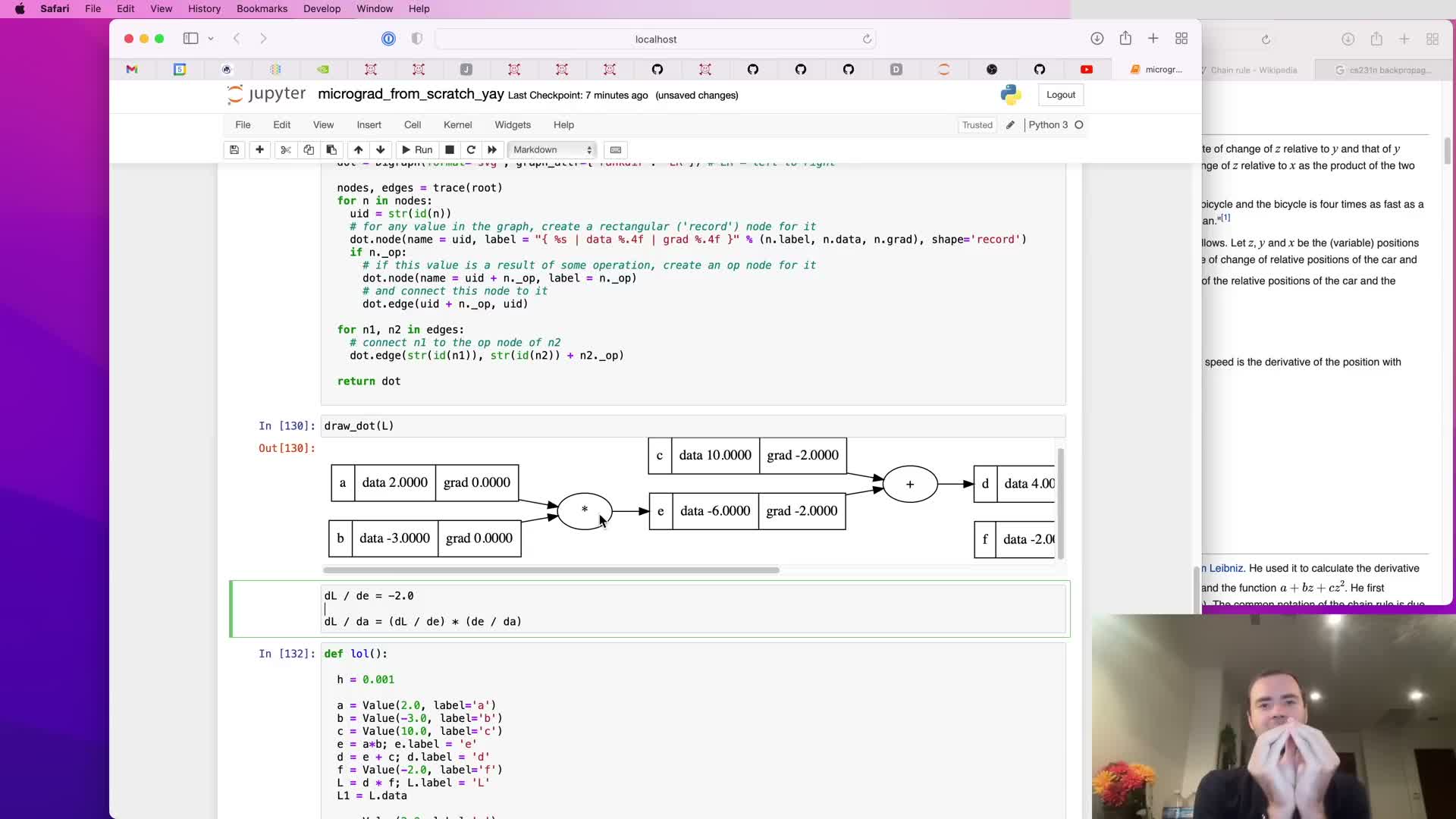
Backpropagation through multiplication nodes is extended to compute gradients for leaf inputs a and b by multiplying upstream gradients by local derivatives (∂e/∂a = b, ∂e/∂b = a).
Illustration:
- The example graph derives a.grad = 6 and b.grad = -4 algebraically and confirms these values numerically with finite differences.
General pattern:
- At each node, multiply incoming gradient by the node’s local Jacobian entries and accumulate into operand gradients.
This validates that reverse-mode differentiation via local chain-rule multiplications yields correct partial derivatives for all leaves.
Using gradient information to perform a parameter update
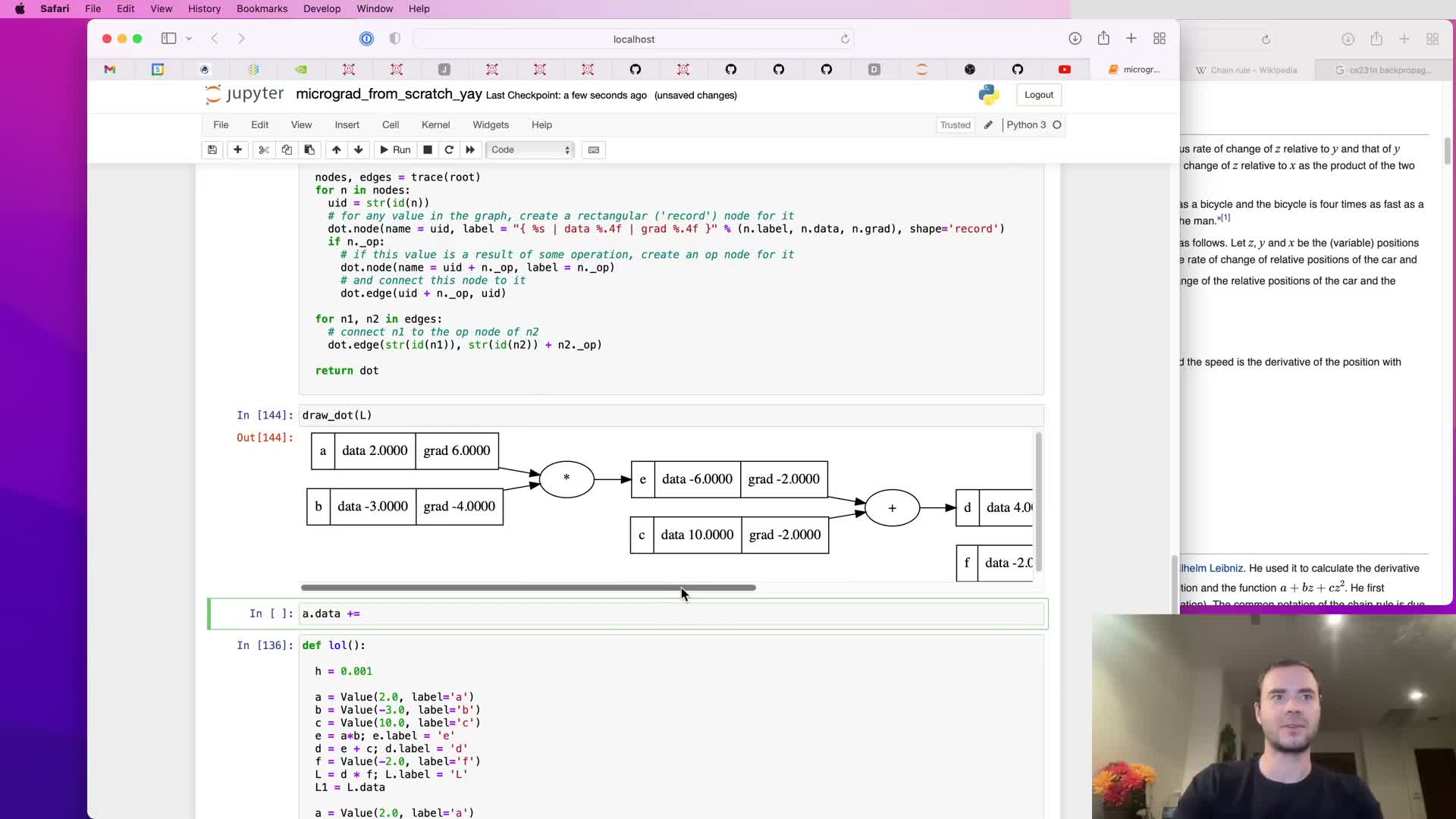
Once gradients for leaf nodes (parameters) are available, a small parameter update step is demonstrated.
Update rule:
- Parameters are nudged by the gradient scaled by a step size (learning rate): parameter -= lr * grad.
Notes:
- Moving parameters in the positive gradient direction increases the output; when minimizing a loss, updates move opposite to the gradient sign.
- A single-step update illustrates how gradient information becomes actionable and foreshadows iterative training loops used later.
Mathematical model of a neuron and activation function choice
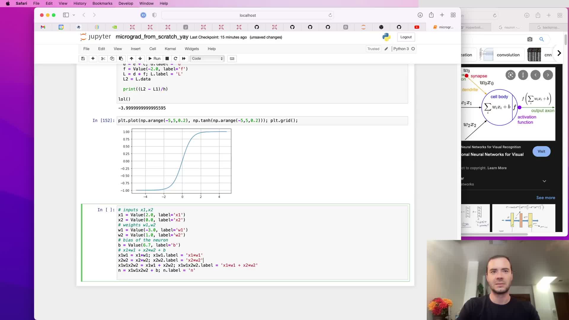
A neuron’s forward computation is defined and motivated:
Definition:
-
output = tanh(w · x + b) — a weighted sum of inputs plus bias followed by a nonlinearity.
Interpretation:
- Inputs and weights interact multiplicatively at synapses.
- Biases shift activation thresholds.
- The tanh activation squashes output into [-1, 1], introducing saturation useful for representation learning.
Implementation decision:
-
tanh can be implemented as a composite of exponentials or as a single primitive if its local derivative is supplied; this choice affects clarity and convenience in the educational implementation.
Implementing tanh as a Value operation and its backward rule
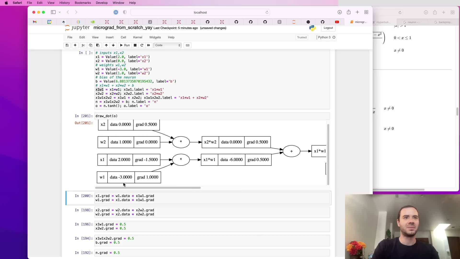
Tanh is implemented as a custom Value operation with its own local backward rule:
Local derivative:
- d/dx tanh(x) = 1 - tanh(x)^2.
Implementation detail:
- The returned Value stores the computed tanh output so the backward closure can reference it efficiently during backpropagation.
- The backward closure multiplies the incoming gradient by (1 - output^2) and accumulates it into the child node’s .grad.
Verification:
- The computed gradient is checked numerically to confirm correctness and to demonstrate composed forward passes including tanh behave as expected.
Automating local backward logic by storing closures in nodes
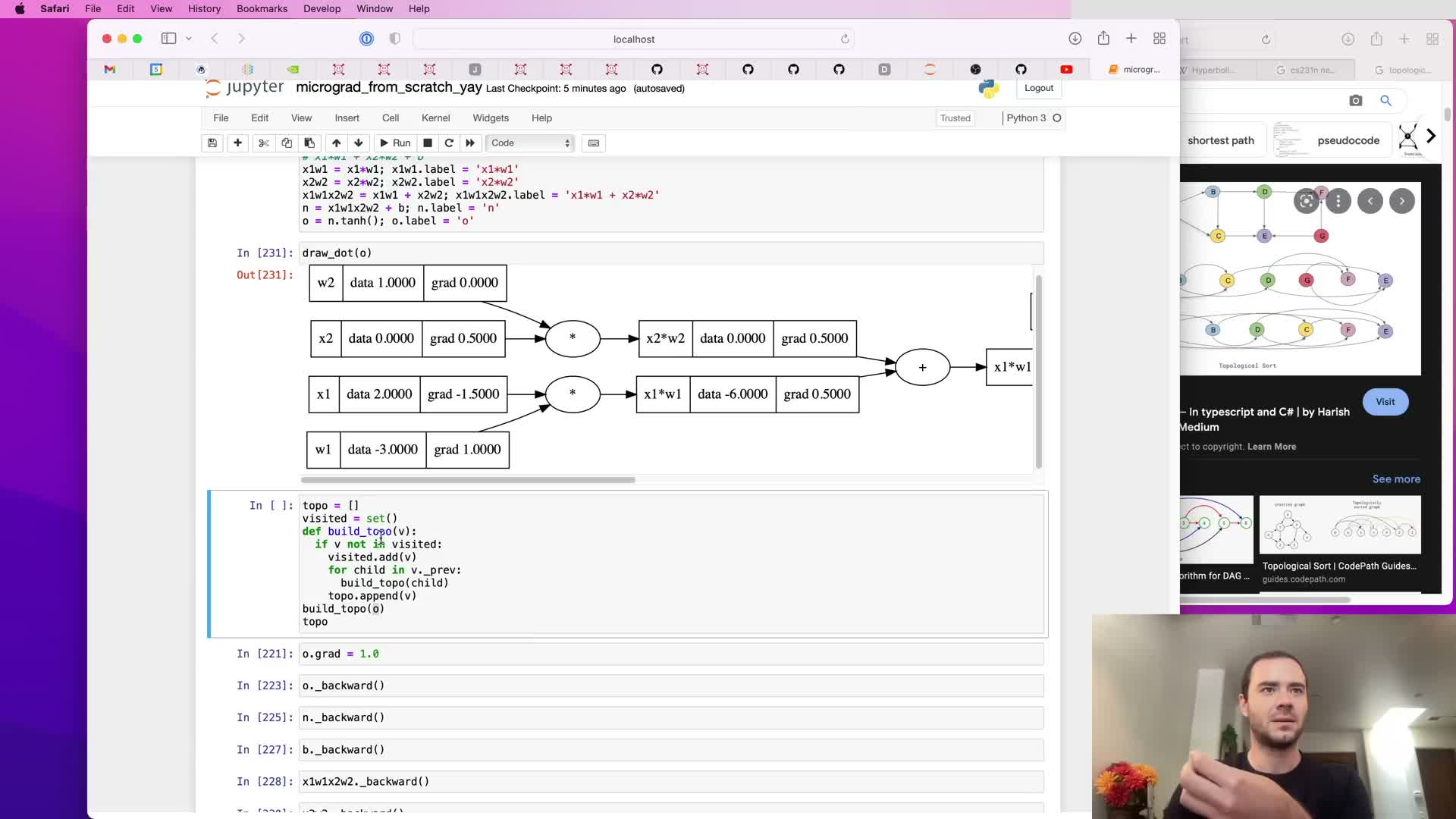
Each Value node stores a small function closure (_backward) that performs the node-specific local chain-rule propagation into operand gradients when invoked.
Mechanics:
- For primitives like addition, multiplication, and tanh, _backward captures runtime values (operand data or tanh output) and encodes the local derivative formula.
- During the global backward traversal, the algorithm simply invokes each node’s _backward closure without hard-coding operator-specific behavior.
Design benefit:
- Local differentiation logic is encoded next to forward computation while the global backward routine remains generic and uniform.
Topological sorting and implementing Value.backward
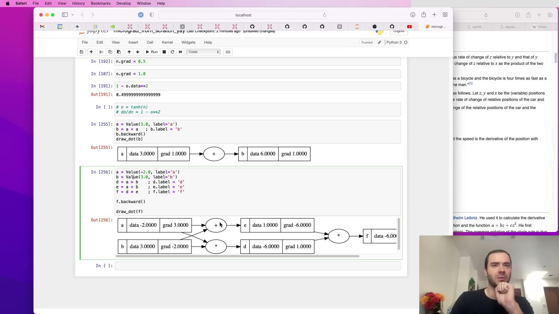
Automatic backward execution requires visiting nodes in an order where children are processed before parents; this is achieved via a topological sort of the computation DAG.
Algorithm:
- Recursively traverse children to build a topological ordering of nodes.
- Set the final output’s .grad = 1.0 to seed the pass.
- Iterate the topo list in reverse and invoke each node’s _backward closure to accumulate gradients.
Result:
- Guarantees correct reverse-mode propagation for arbitrary DAGs and encapsulates the entire backward evaluation in a single .backward() call.
Gradient accumulation bug on reused variables and the accumulation fix
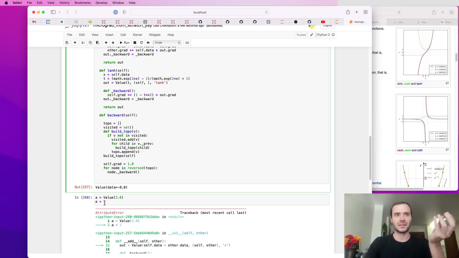
A subtle bug arises when a variable is used multiple times (e.g., b = a + a) and backward implementations overwrite operand gradients instead of accumulating them.
Correct behavior:
- Contributions from multiple downstream paths must be summed, so backward routines must use += when updating operand .grad fields.
Fix:
- Change assignments to accumulations, re-run tests, and verify cases like a + a produce the expected factor-of-two gradients.
Lesson:
- Proper gradient initialization and additive accumulation are essential in reverse-mode AD to reflect multiple gradient paths correctly.
Convenience wrappers for numeric constants and right-side operations
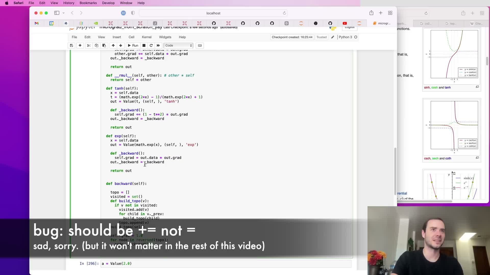
To allow mixing Value objects with Python numeric literals (e.g., a + 1 or 2 * a), the operator implementations wrap non-Value operands into Value instances automatically.
Additional API ergonomics:
- Implement right-hand operator fallbacks (e.g., __rmul__) so Python calls into Value when native numeric types are on the left.
Benefit:
- The Value API behaves similarly to numeric types and lets users write expressive mathematical code without manually wrapping constants, while preserving forward and backward semantics.
Adding exp/power, division, subtraction primitives and equivalence of decomposed tanh
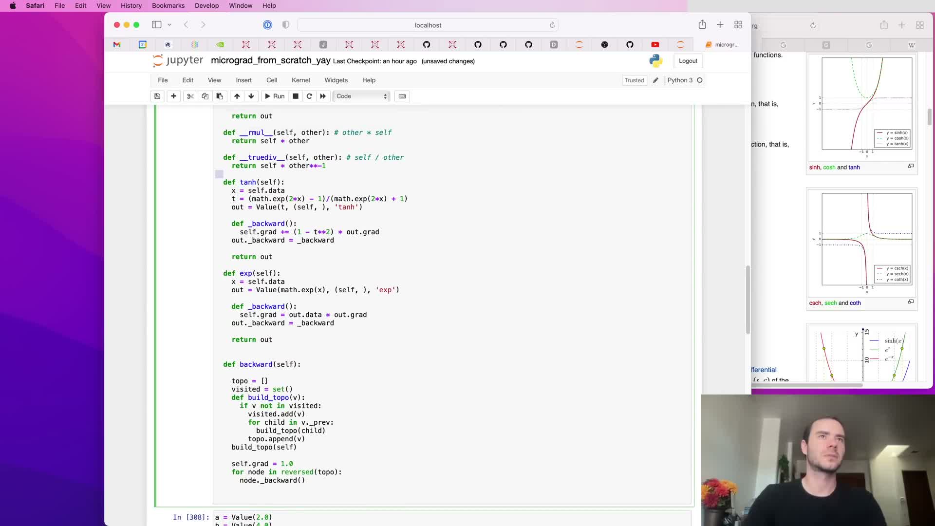
Exponentiation and related operations are implemented along with composition strategies to avoid duplicating logic:
Implementations:
-
exp and power operations: forward computations plus local backward rules (d/dx e^x = e^x; power rule for x^n).
-
Division implemented as multiplication by a power of -1: a / b = a * b**-1 so reciprocal behavior reuses the power primitive.
-
Subtraction and negation composed from primitives (negation as multiplication by -1, subtraction as addition of a negation).
Validation:
- Implementing tanh as a composite of exponentials produces identical forward values and backward gradients as the single-operation tanh version, demonstrating correctness and modularity of composed operations.
Neural modules: neuron, layer, and MLP abstractions matching common APIs
A Neuron class is implemented with weight and bias Value parameters and a call operator that computes dot product + bias followed by an activation.
Higher-level modules:
-
Layer: a collection of Neuron instances evaluated in parallel.
-
MLP: chains Layers sequentially to form multilayer perceptrons.
API conventions:
- Each module exposes a parameters() method that aggregates leaf Value parameter instances so external optimization code can iterate them.
- The design mirrors mainstream frameworks (e.g., PyTorch’s nn.Module) to make the micrograd API familiar in concept.
This encapsulation separates forward computation from parameter management and simplifies building networks of arbitrary depth and width.
Dataset construction, loss definition (MSE), and computing gradients for training
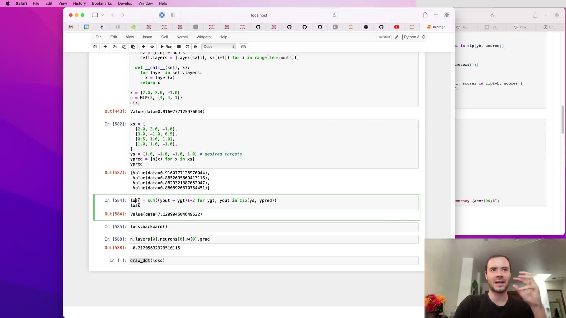
A small toy dataset of input vectors and scalar targets is created to demonstrate supervised learning with the MLP.
Loss and training:
- Run the MLP on each example to produce predictions.
- Define mean squared error (MSE) as the average squared difference between predictions and targets, producing a single scalar loss.
- Calling loss.backward() populates gradients for all parameter Values across the examples because the loss graph chains back through each forward evaluation.
Use of gradients:
- Inspecting parameter .grad values indicates whether increasing a weight will increase or decrease the loss and thus guides updates.
Parameter update loop, learning rate selection, and iterative optimization
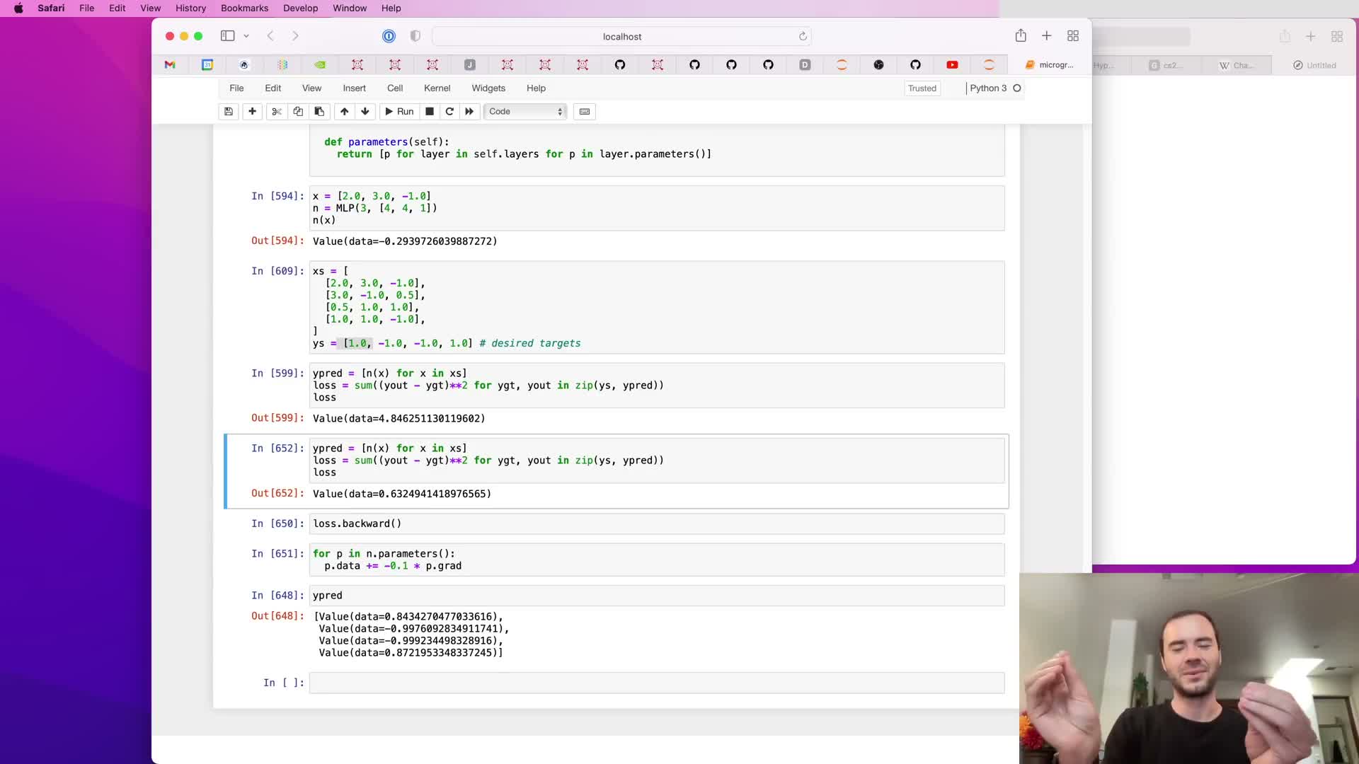
A training loop repeatedly:
- Performs forward passes to compute predictions.
- Computes the scalar loss (MSE).
- Calls .backward() to populate gradients.
- Updates parameters by subtracting lr * grad for each parameter.
Observations:
- Different learning rates affect convergence speed and stability: too small = slow progress; too large = instability or exploding loss.
- The shown process is basic stochastic gradient descent (SGD) with full-batch updates in the toy example, and it generalizes to mini-batches and more advanced optimizers.
Repeated forward-backward-update cycles progressively reduce loss and improve predictions on the toy task.
Zeroing gradients across iterations and consequences of forgetting to zero
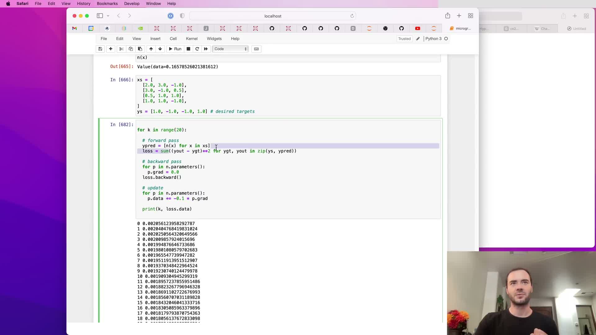
Gradients must be reset to zero prior to each backward pass because .grad updates accumulate via +=.
Pitfall:
- Forgetting to zero gradients causes accumulation across iterations and scales updates unpredictably, producing incorrect or unstable training dynamics.
Fix:
- Iterate over parameters and set p.grad = 0 before calling backward() each iteration.
This mirrors standard practice in production frameworks and is essential for correct iterative optimization.
Comparison with PyTorch implementation details and registering custom ops
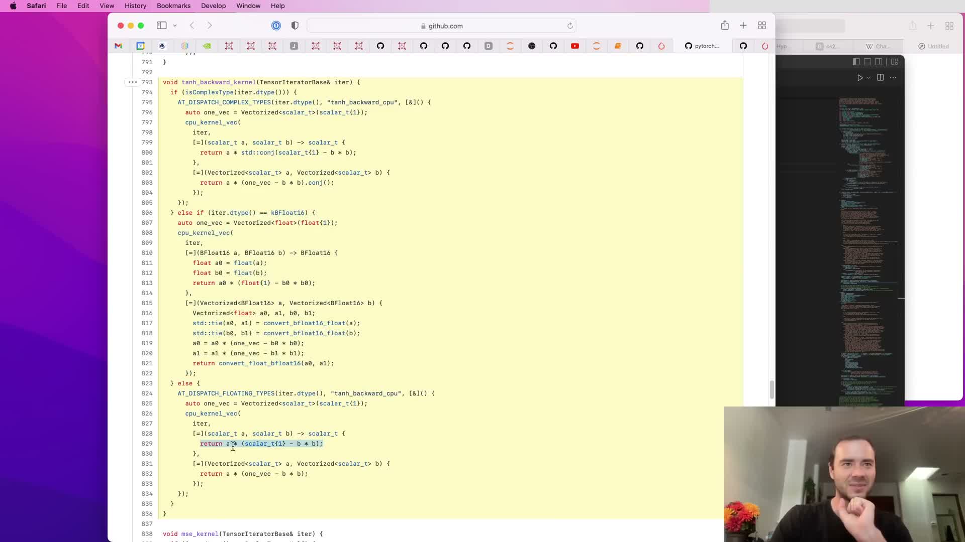
Compare micrograd’s scalar Value abstraction to production tensors (e.g., PyTorch):
Comparative points:
-
PyTorch generalizes the same autograd ideas to n-dimensional tensors for parallel, efficient CPU/GPU computation and exposes similar data and grad attributes and a backward API.
- The lecture inspects where tanh backward is implemented in PyTorch’s C++/CUDA kernels and shows how to register custom ops by providing forward and backward implementations that match micrograd’s conceptual contract.
Conclusion:
- Micrograd’s small, explicit design scales conceptually to production libraries, while production code adds complexity for device support, datatypes, and performance engineering.
Summary of principles: expressions, loss, backprop, and gradient descent
Recap and pipeline summary:
Core ideas:
- Neural networks are mathematical expressions parameterized by weights mapping inputs to outputs; a scalar loss measures performance and is minimized via gradient-based updates.
-
Backpropagation (reverse-mode differentiation) computes exact derivatives of the loss with respect to all parameters by chaining local derivatives at each operation.
- The micrograd implementation contains the mathematical essentials of larger frameworks; the remaining differences are engineering for tensors, devices, and scale.
End-to-end pipeline:
- Define model.
- Compute forward pass (predictions).
- Compute scalar loss.
- Backpropagate gradients via .backward().
- Update parameters (parameter -= lr * grad).
- Iterate.
This ties together the lecture: the tiny engine exposes every moving part so the learner understands both theory and practice before moving to production systems.
Enjoy Reading This Article?
Here are some more articles you might like to read next: