Karpathy Series - Building Makemore
- MakeMore is a character-level generator that learns to produce strings similar to a provided dataset.
- Load the raw dataset into a list of strings and compute basic statistics before modeling.
- A character-level language model predicts the next character in a sequence and can be implemented with models ranging from bigrams to transformers.
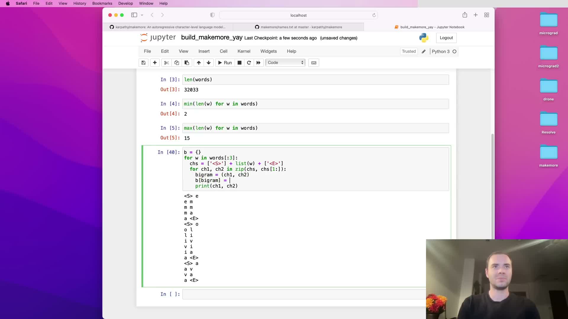
- Bigrams are extracted by sliding a two-character window over sequences augmented with explicit start and end tokens.
- Accumulate bigram frequencies in a dictionary and then represent them as a 2D count matrix for efficient computation.
- Build character-to-index and index-to-character lookup tables, populate the count matrix, and visualize bigram statistics.
- Special start/end token placement can create wasted zero rows/columns; use a single sentinel and offset indices to eliminate redundancy.
- Sample sequences by normalizing a row of counts into probabilities and drawing with torch.multinomial using a seeded generator for deterministic randomness.
- Iterative sampling from a bigram model produces limited-quality outputs because context is restricted to one previous character; uniform baselines illustrate the learned signal.
- Precompute a probability matrix P by normalizing the counts tensor once and use it for fast sampling instead of repeated per-step normalization.
- Respect broadcasting semantics and prefer keepdim to preserve intended shapes; use in-place ops to reduce allocations.
- Measure model quality with the likelihood and its log transforms, using negative log-likelihood as a loss to minimize.
- Prevent infinite loss from zero-probability events by applying additive smoothing to counts before normalization.
- Cast bigram prediction as a supervised neural network task by compiling input-target integer pairs from all bigrams.
- Use one-hot encoding to convert integer inputs to float vectors and implement the linear layer as a weight matrix evaluated by matrix multiplication.
- Interpret linear outputs as logits, apply softmax to obtain probabilities, and compute NLL loss by indexing predicted probabilities at target positions.
- Compute gradients via automatic differentiation and update parameters with gradient descent to minimize the NLL loss.
- Gradient-based training on the full bigram dataset converges to a parameter matrix that is equivalent to the count-based table; initialization and regularization connect to smoothing, and the neural model can be used for sampling.
MakeMore is a character-level generator that learns to produce strings similar to a provided dataset.

MakeMore is a character-level language generator that learns from a corpus of example strings and produces new strings that resemble the training data in style and structure.
The example dataset is a large names file of roughly 32,000 entries, and training on this data yields novel, name-like outputs.
Because the model operates at the character level, every training example is a line treated as a sequence of characters, and repeated sampling from the trained model generates unique yet name-like tokens.
Use cases include creative generation — for example, inventing candidate names or other short strings that follow learned character patterns.
Load the raw dataset into a list of strings and compute basic statistics before modeling.
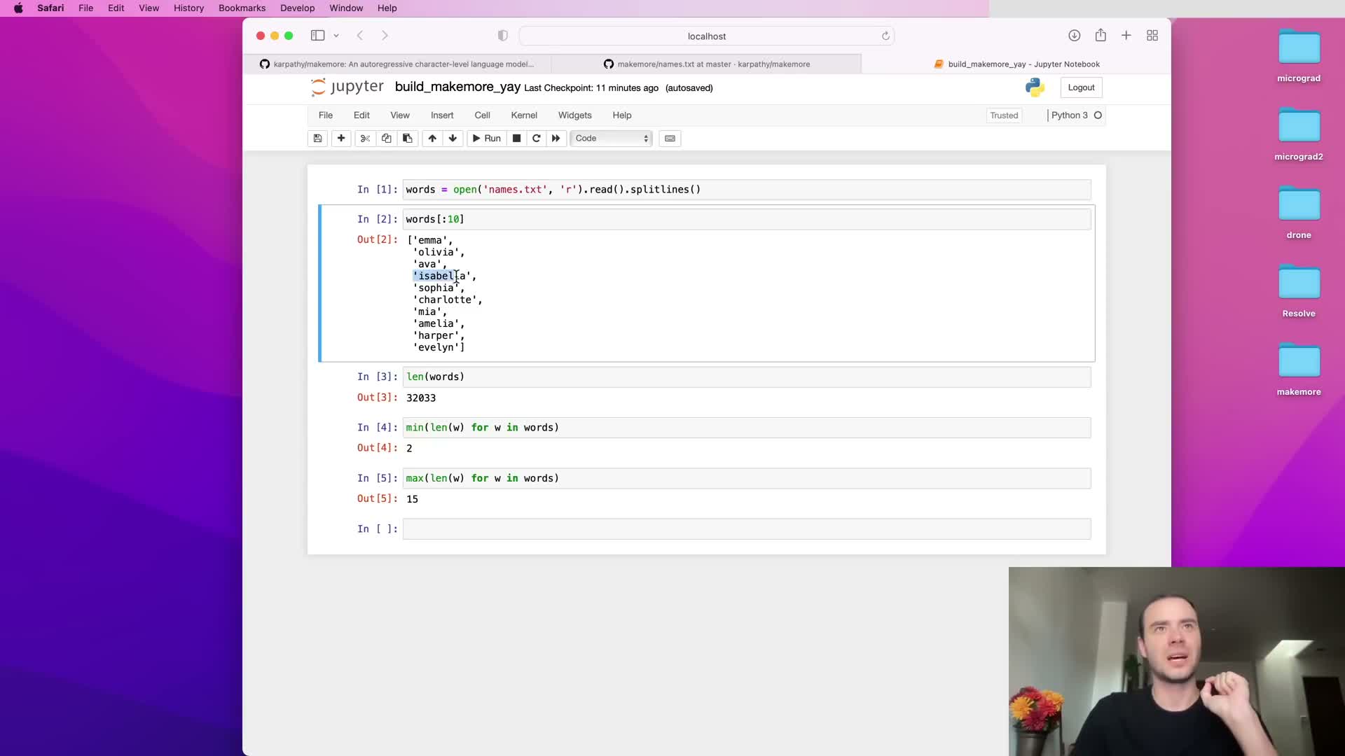
The raw text file is opened and read into a single string and then split into individual lines to form a list of word strings.
Basic exploratory statistics to compute and record include:
- Total number of words (≈32,000)
- Shortest word length
-
Longest word length
These statistics guide downstream decisions such as vocabulary size and sequence length handling.
Inspecting the first few list elements also reveals potential frequency ordering, which can affect sampling priors and preprocessing assumptions.
Recording these metadata ensures reproducible preprocessing and informs later choices for tokenization and model capacity.
A character-level language model predicts the next character in a sequence and can be implemented with models ranging from bigrams to transformers.
A character-level language model treats each string as a sequence of characters and learns the conditional distribution of the next character given a context.
Implementations range from simple statistical models (e.g., bigrams) to multilayer perceptrons, recurrent neural networks (RNNs), and modern transformers.
Key distinctions across architectures:
- Amount of preceding context they condition on
- Parameterization of the conditional distribution
Building progressively from bigrams up to a character-level transformer clarifies how complexity and expressivity increase while preserving the same prediction and training objectives.
Character-level models are a compact setting to explore language-modeling mechanics before scaling to word-level or multimodal architectures.
Bigrams are extracted by sliding a two-character window over sequences augmented with explicit start and end tokens.
A bigram dataset is formed by sliding a window of two consecutive characters through each augmented sequence.
Augmentation is done by prepending a start token and appending an end token so that boundary events (start→first, last→end) become explicit training examples.
In code, the Python zip trick (zipping a string with its offset-by-one copy) produces consecutive character pairs for each word efficiently.
Including the special tokens ensures the model learns initial and terminal character statistics.
Each original string therefore yields multiple training examples equal to its length plus one (for the final end token), providing many local-context examples for statistical estimation.
This bigram representation is the foundation for both counting-based statistics and neural formulations.
Accumulate bigram frequencies in a dictionary and then represent them as a 2D count matrix for efficient computation.
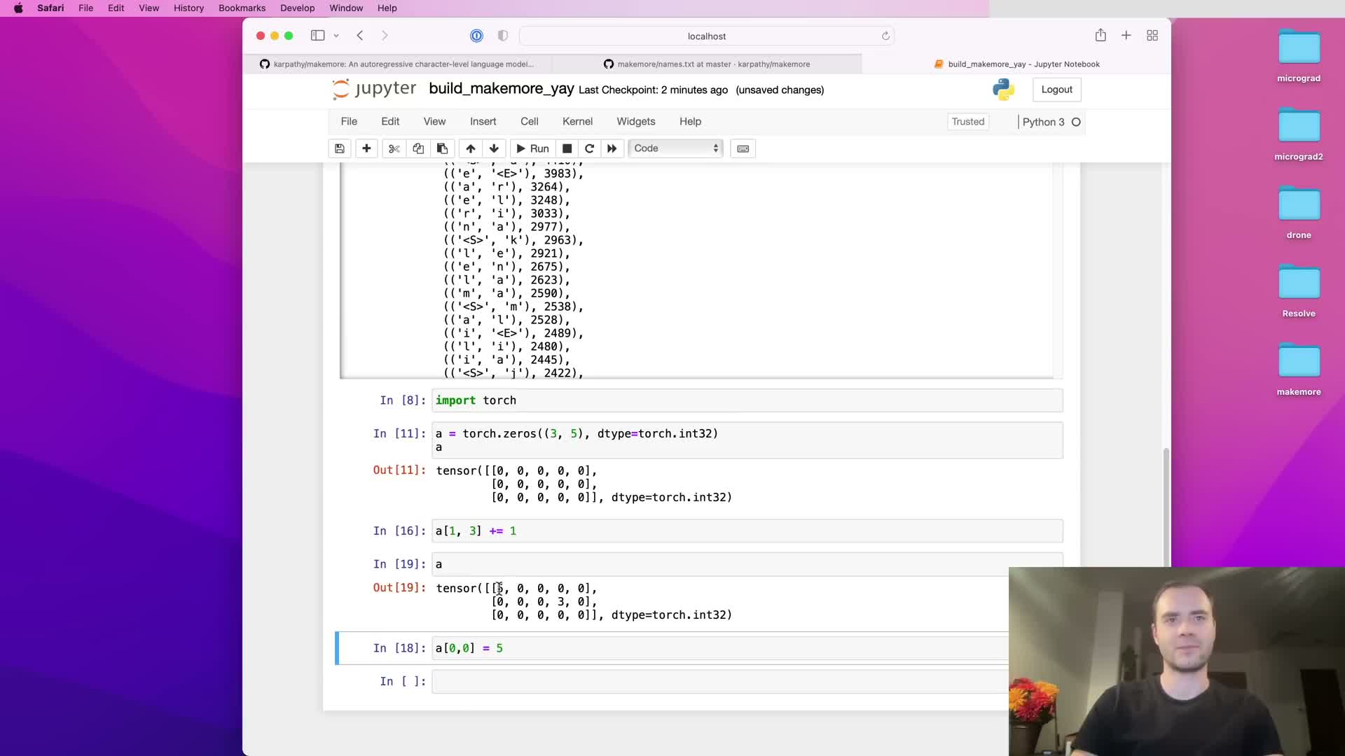
Bigram occurrences can be counted in a dictionary keyed by (char1, char2) tuples with integer counts incremented for every observed pair; this gives a simple maximum-likelihood estimate of conditional counts.
For computational efficiency and vectorized operations, convert the dictionary counts into a two-dimensional numeric array (matrix):
- Rows index the first character
- Columns index the second character
A numeric tensor representation (e.g., a PyTorch tensor) allows efficient indexing, arithmetic, and downstream normalization into probability distributions.
Using an integer data type for counts preserves exactness prior to conversion to floating point for probabilistic computations.
Build character-to-index and index-to-character lookup tables, populate the count matrix, and visualize bigram statistics.
Construct an ordered vocabulary by concatenating the dataset and taking the sorted set of characters, then enumerate this list to create:
- s2i (string-to-index) mapping
-
i2s (index-to-string) inverse for reconstruction
Use these mappings to translate character bigrams to integer indices and increment the corresponding entries in the 2D count matrix.
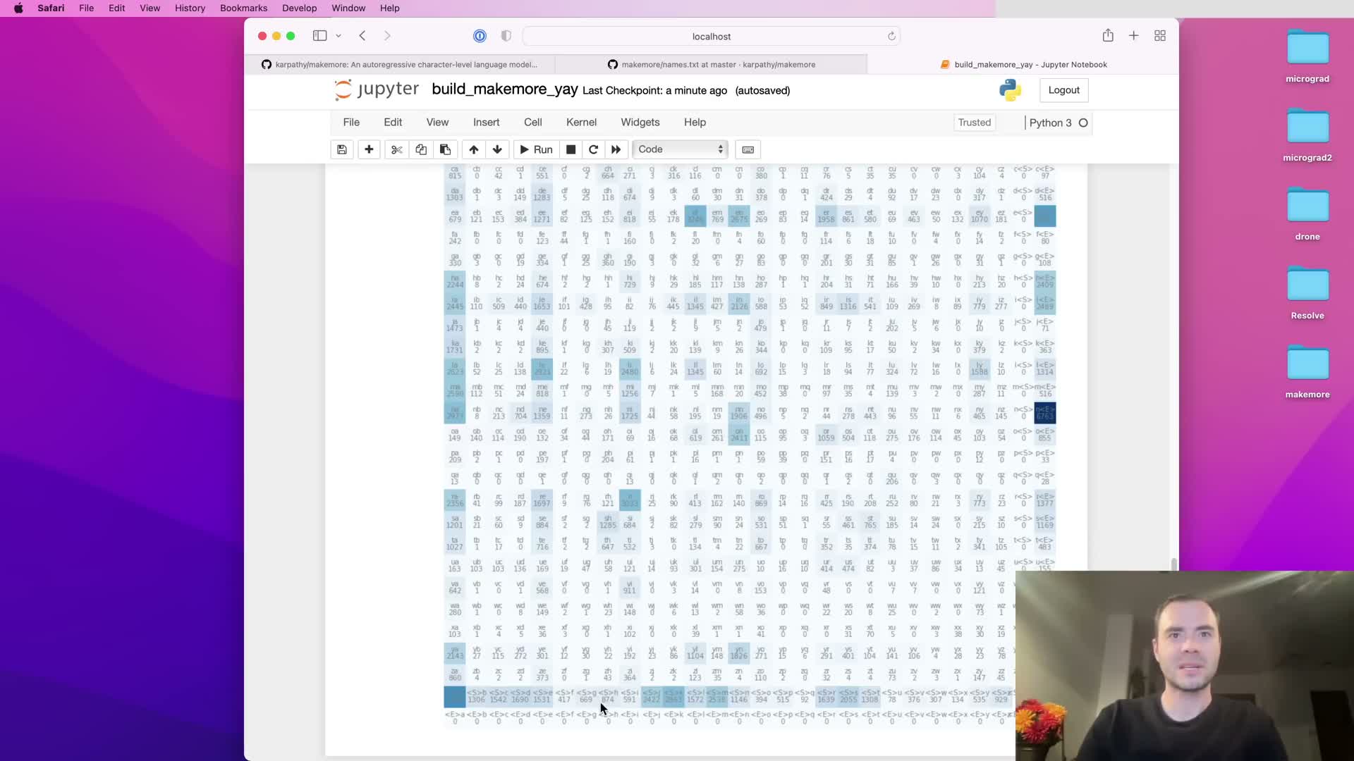
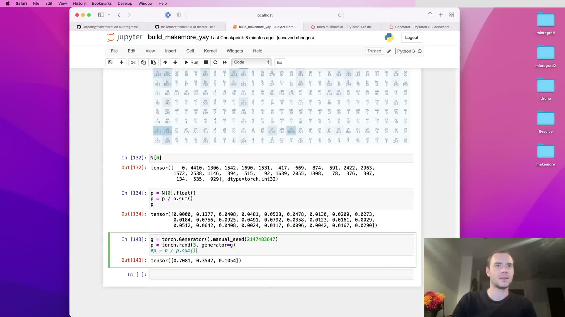
Visualization (for example with matplotlib) of the 2D matrix provides diagnostics that expose frequent and rare transitions and highlights anomalies or structural patterns in the dataset.
When plotting, convert tensor elements to native Python numbers (e.g., using .item()) as framework-specific scalar objects may not be directly plottable.
Special start/end token placement can create wasted zero rows/columns; use a single sentinel and offset indices to eliminate redundancy.
When start and end tokens are represented as distinct indices and placed only at sequence boundaries, entire rows or columns of the count matrix become identically zero because those transitions are impossible by construction.
A compact alternative is to replace the two separate tokens with a single sentinel (for example, a dot) at index 0 and offset regular characters by +1. This yields an N×N matrix (for the names example, 27×27) with no structurally guaranteed empty rows/columns.
Benefits of this compacting:
- Reduces wasted storage
- Simplifies indexing logic for sampling and training
Ensure the sentinel is handled consistently across preprocessing and sampling to avoid subtle out-of-range or impossible-transition bugs.
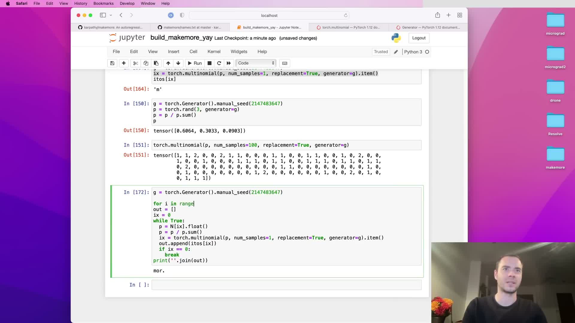
Sample sequences by normalizing a row of counts into probabilities and drawing with torch.multinomial using a seeded generator for deterministic randomness.
Sampling the next character from the bigram model proceeds as follows:
- Select the row of counts corresponding to the current character.
- Convert that integer vector to floating point and normalize by its sum to create a probability distribution.
- Sample an index according to that distribution.
In PyTorch, torch.multinomial performs multinomial draws and accepts a generator object seeded for deterministic reproducibility so repeated runs produce identical samples when required.
Set replacement appropriately (usually True) to allow repeated draws of the same index within a sampling batch.
Map sampled indices back to characters via i2s to yield the generated sequence; termination is signaled by sampling the sentinel index.
Iterative sampling from a bigram model produces limited-quality outputs because context is restricted to one previous character; uniform baselines illustrate the learned signal.
Repeated sampling by starting at the sentinel and drawing successive characters until the sentinel appears yields outputs that are superficially name-like but often nonsensical — reflecting the intrinsic limitation of bigram models, which condition only on the immediately preceding character.
A uniform sampling baseline (equal probability for each character) demonstrates how much empirical bigram probabilities have learned structure: the trained bigram model typically outperforms uniform, but still produces poor global coherence because longer-range dependencies are ignored.
This comparison highlights the need for larger-context models (n-grams with n>2, RNNs, transformers) to capture morphological and phonotactic patterns beyond local adjacency.
Empirical inspection of generated samples is a practical, qualitative diagnostic for model adequacy.
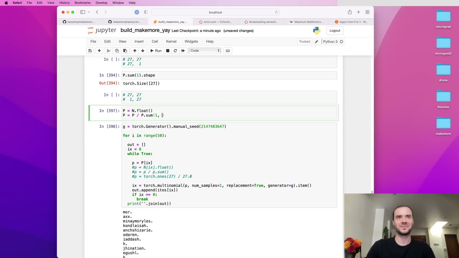
Precompute a probability matrix P by normalizing the counts tensor once and use it for fast sampling instead of repeated per-step normalization.
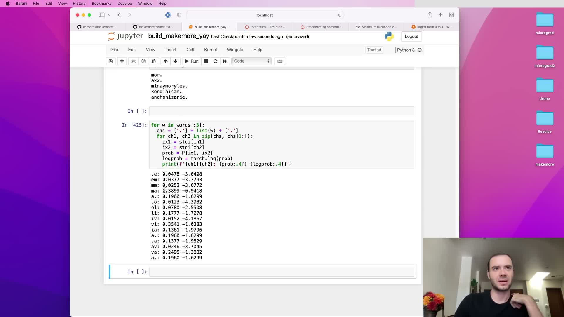
Repeated per-step conversion of count rows to probabilities is inefficient and duplicates work.
Instead:
- Compute a floating-point copy of the entire count matrix.
- Sum each row to produce a column vector of row totals.
- Divide the count matrix by that column vector to obtain a full P matrix of row-wise conditional probability distributions.
Performing this normalization once up front enables constant-time row lookup during sampling and avoids repeated allocations and numeric conversions.
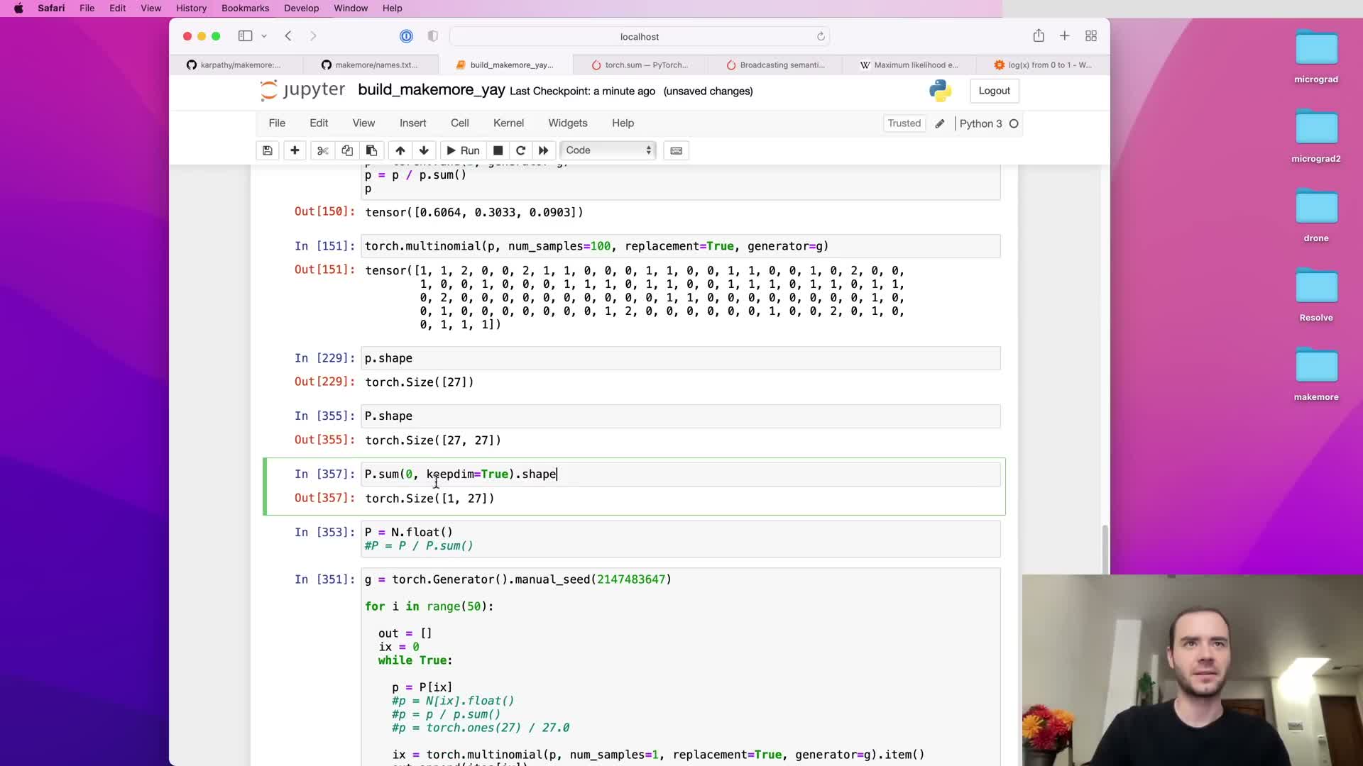
Use torch.sum with the appropriate dimension and keepdim=True to preserve the singleton dimension required for correct broadcasting during division.
Storing P as a float tensor trades some memory for much faster sampling and vectorized evaluation.
Respect broadcasting semantics and prefer keepdim to preserve intended shapes; use in-place ops to reduce allocations.
Broadcasting rules require alignment of tensor shapes starting from trailing dimensions; preserving singleton dimensions via keepdim=True prevents silent creation of undesired row/column orientation when a summed vector is used in elementwise operations.
If a summed vector loses its singleton dimension, it may broadcast as a row rather than a column, yielding column-wise normalization instead of the intended row-wise normalization and producing incorrect probability matrices — a subtle, framework-specific bug.
In-place operations (where supported) reduce memory churn and can be faster than creating new tensors; however, they must be used with an understanding of autograd semantics to avoid interfering with gradient computation.
Careful unit tests or shape assertions are recommended when performing broadcasted normalization to avoid hard-to-find errors.
Measure model quality with the likelihood and its log transforms, using negative log-likelihood as a loss to minimize.

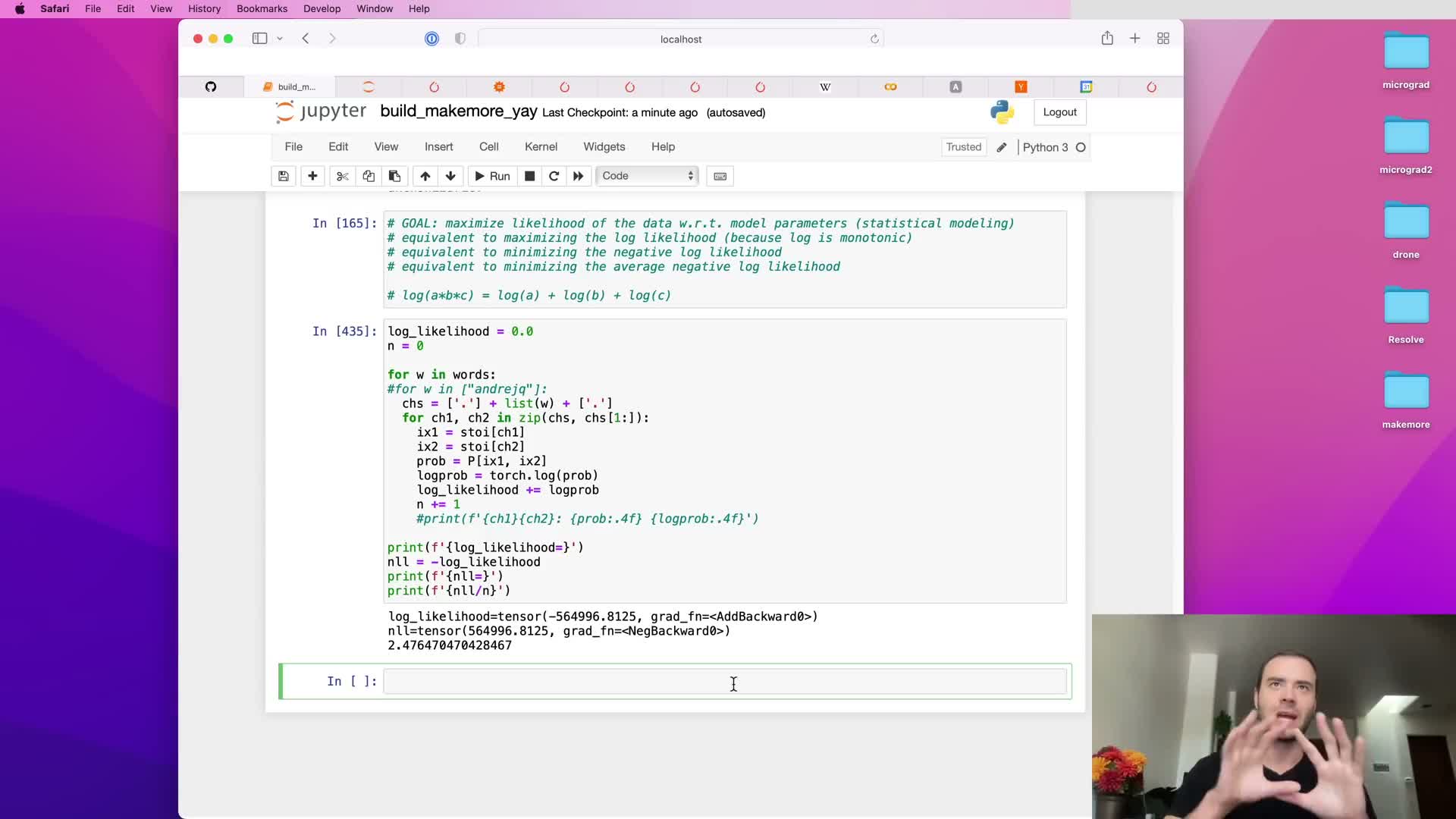
The likelihood of the dataset under the model is the product of predicted probabilities for every observed bigram; the log-likelihood is the sum of the log probabilities, which is numerically more stable and additive across examples.
Define negative log-likelihood (NLL) as the negative of the log-likelihood. NLL is a convenient loss because:
- It maps perfect predictions to zero
- It penalizes improbable predictions with larger positive values
Averaging the NLL across examples yields an interpretable per-example loss metric (e.g., measured in bits or nats depending on log base) that can be minimized during training.
Using the log makes multiplication of many small probabilities tractable and converts maximum-likelihood estimation into a standard minimization objective.
Prevent infinite loss from zero-probability events by applying additive smoothing to counts before normalization.
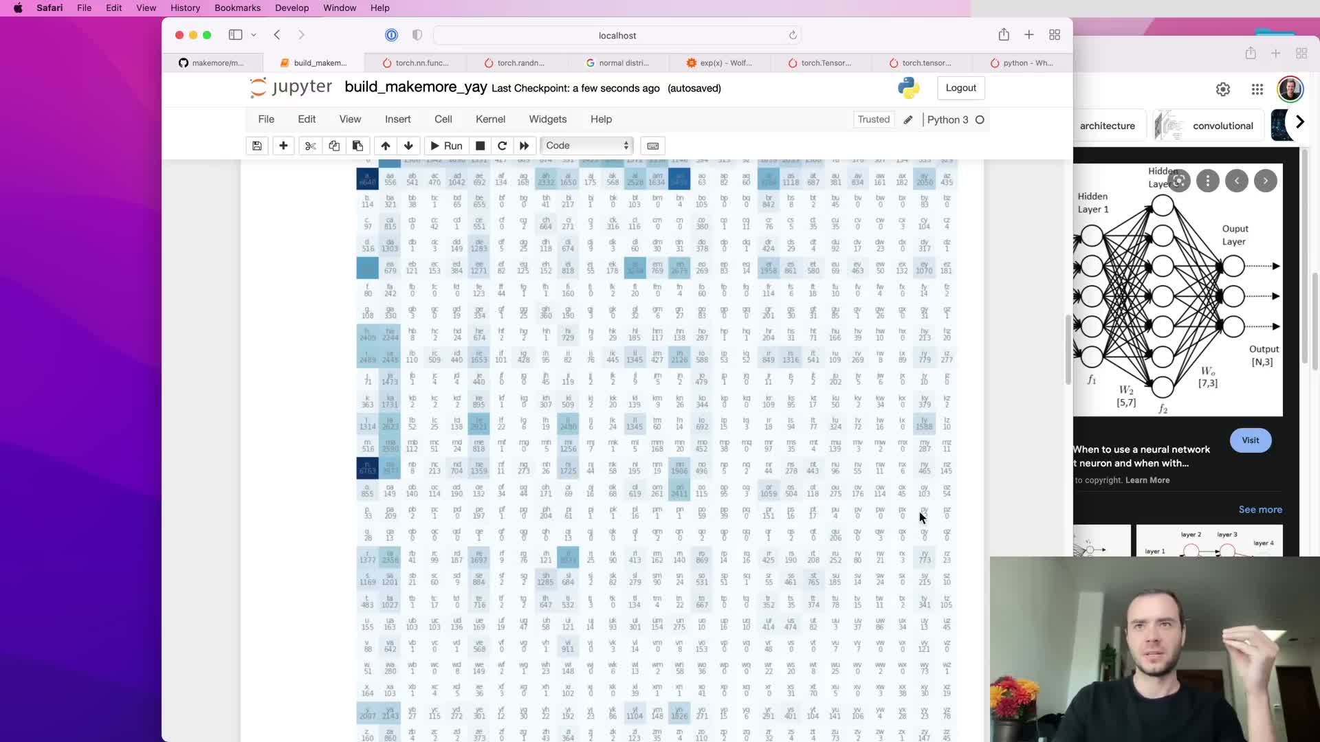
Direct maximum-likelihood counts may assign zero probability to unseen bigrams, which produces log(0) = -infinity and makes the NLL ill-posed on those examples.
Additive smoothing (Laplace smoothing) adds a small positive pseudo-count (commonly 1) to every count cell before normalization, ensuring every bigram has non-zero probability and finite log-loss.
Varying the smoothing constant interpolates between the empirical distribution (small smoothing) and a uniform prior (very strong smoothing); the smoothing choice trades bias for numeric robustness.
Smoothing is especially important when evaluating or generating sequences that may contain low-frequency or previously unseen transitions.
Cast bigram prediction as a supervised neural network task by compiling input-target integer pairs from all bigrams.
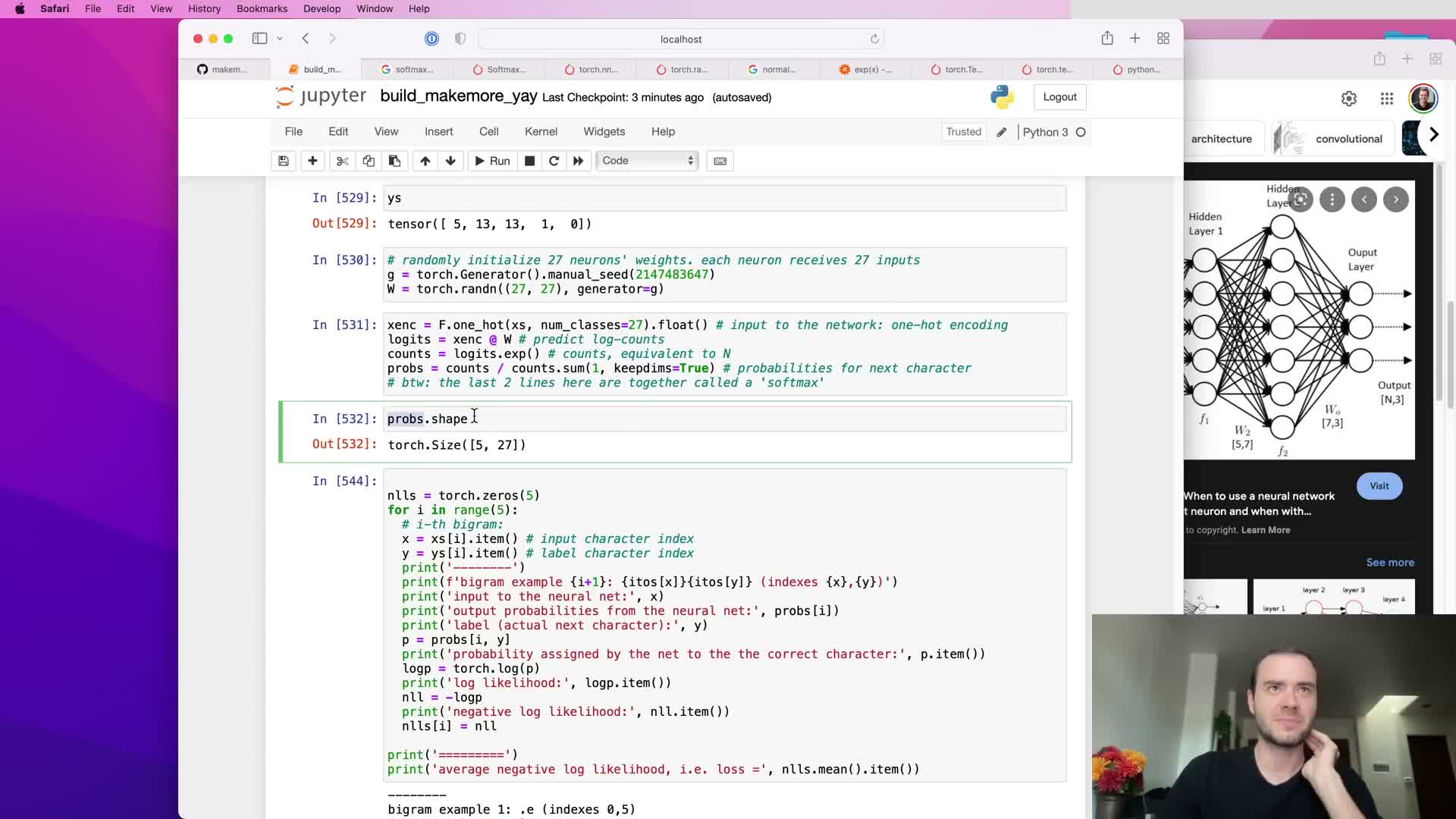
The supervised training dataset consists of:
- Input indices (the first character of each bigram)
-
Target indices (the second character)
Collect these across all augmented sequences so that each bigram becomes a separate training example.
Convert the collected Python lists into framework tensors using constructors that preserve intended integer dtypes (for PyTorch, use torch.tensor with integer dtype semantics).
This formulation enables standard neural training pipelines: batched forward passes, differentiable losses computed on predicted distributions, and backpropagation to optimize parameters.
Treating bigram prediction as a classification task over the token vocabulary frames the problem for gradient-based optimization.
Use one-hot encoding to convert integer inputs to float vectors and implement the linear layer as a weight matrix evaluated by matrix multiplication.

Integer token indices are transformed into one-hot vectors of length equal to the vocabulary size so a linear layer (matrix multiply plus optional bias) can process them as real-valued inputs.
Note: One-hot encoding APIs often return an integer dtype by default, so an explicit cast to float is typically required before feeding vectors into a neural layer.
The linear layer weight matrix W with shape (vocab_size, hidden_or_output_dim) can be multiplied with the one-hot vectors; when inputs are one-hot, multiplication is equivalent to selecting the corresponding row of W, so the matrix representation generalizes the lookup table.
Initializing weights with small random values (e.g., a normal distribution) provides symmetry breaking for gradient-based learning.
Interpret linear outputs as logits, apply softmax to obtain probabilities, and compute NLL loss by indexing predicted probabilities at target positions.

A neural net linear layer outputs real-valued logits for every class which are exponentiated and normalized (softmax) to produce a valid probability distribution over next tokens.
The softmax operation is the differentiable composition of exp and row-wise normalization and maps arbitrary logits to non-negative numbers that sum to one.
For loss calculation:
- Select the probability assigned to the true target class for each example by indexing the probability matrix at row indices (batch positions) and column indices (targets).
- Convert these to log probabilities and average the negative logs to produce the NLL.
This vectorized indexing approach enables efficient batch loss computation without explicit Python loops.
Compute gradients via automatic differentiation and update parameters with gradient descent to minimize the NLL loss.

Automatic differentiation frameworks build a computational graph during the forward pass and populate gradient tensors after invoking backward() on the scalar loss, making derivatives of the NLL with respect to model parameters available automatically.
Before backward propagation, parameter gradients are typically zeroed or set to None to avoid accumulation from previous iterations; after loss.backward(), each parameter’s .grad field contains its gradient.
Parameter updates are implemented as in-place operations on parameter data, for example:
- w.data -= learning_rate * w.grad
Gradient clearing is performed before the next forward-backward cycle. Iterating this loop reduces the average NLL and shapes logits so that exponentiated and normalized outputs match empirical bigram frequencies.
Gradient-based training on the full bigram dataset converges to a parameter matrix that is equivalent to the count-based table; initialization and regularization connect to smoothing, and the neural model can be used for sampling.
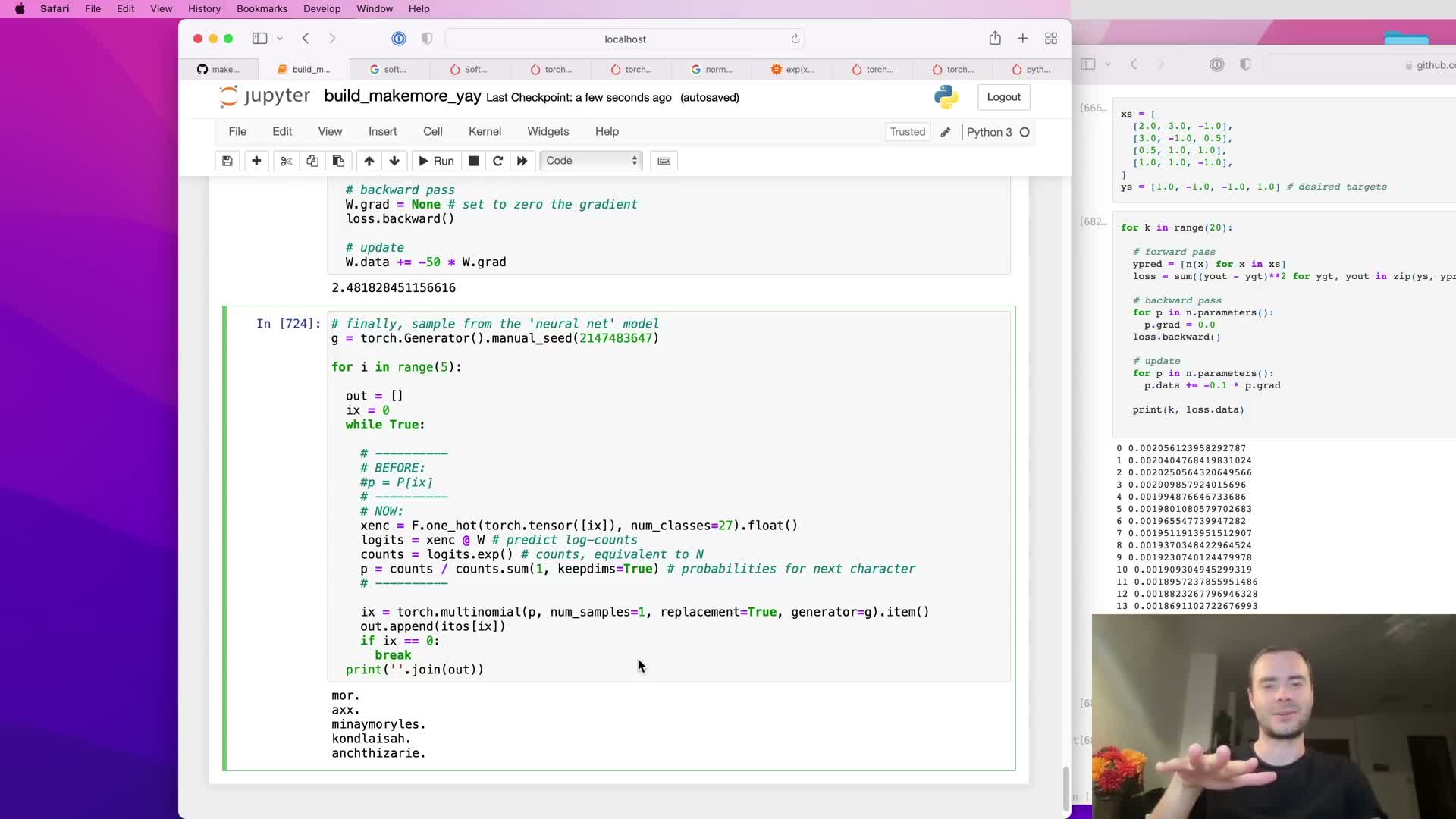
When the neural linear model is trained with NLL on the entire bigram dataset, the learned weight matrix (after exponentiation) reproduces the relative frequencies captured by the explicit count table — gradient-based optimization recovers the maximum-likelihood solution that counting produced.
Practical notes:
- Initializing the weight matrix to zeros yields uniform logits and therefore uniform probabilities, which is equivalent to very strong additive smoothing.
- Adding an L2 penalty on weights acts as a regularizer that biases weights toward zero and increases distributional smoothness.
The trained neural model supports deterministic or seeded probabilistic sampling by computing logits for the current token, applying softmax to obtain P, and drawing the next token from that distribution.
This neural formulation generalizes straightforwardly to larger contexts and more complex architectures where explicit table counting becomes infeasible.
Enjoy Reading This Article?
Here are some more articles you might like to read next: