Karpathy Series - Bulding Makemore Part 2 - MLP
- Recap of bigram model and limitations of single-character context
- Context length causes exponential growth in n-gram tables
- Adopt a multilayer perceptron language model following Bengio et al. 2003
- Token embeddings: low-dimensional learned representations for vocabulary items
- Embedding-based generalization enables transfer across unseen n-grams
- Network architecture: embedding lookup, hidden layer, output softmax
- Model parameters are optimized end-to-end with backpropagation
- Construct dataset using sliding context windows and block size
- Embedding lookup vs one-hot multiplication: equivalence and dtype care
- Batch embedding via advanced indexing: embedding entire x tensor at once
- Concatenation and reshaping: preparing embeddings for a linear hidden layer
- use of unbind and cat for generic concatenation across variable block size
- Tensor view/reshape and underlying storage enable zero-copy reinterpreting
- Hidden layer computation, nonlinearity, and broadcasting of biases
- Final linear layer, softmax, and negative log-likelihood loss
- use of torch.nn.functional.cross_entropy for efficiency and numerical stability
- Training loop mechanics: zeroing gradients, backward pass, and parameter update
- Mini-batch stochastic gradient descent: sampling indices and reducing computation
- Learning rate selection with an exponential sweep (LR finder)
- Train/validation/test splits and roles of each split
- Functionized dataset construction, shuffling, and split sizes
- Scaling model capacity: hidden layer increase and underfitting diagnosis
- Visualizing 2D character embeddings reveals learned structure
- Increase embedding dimensionality and further training to reduce loss
- Sampling from the trained model using autoregressive generation
- Provision of executable Colab notebooks to reproduce and tinker
Recap of bigram model and limitations of single-character context
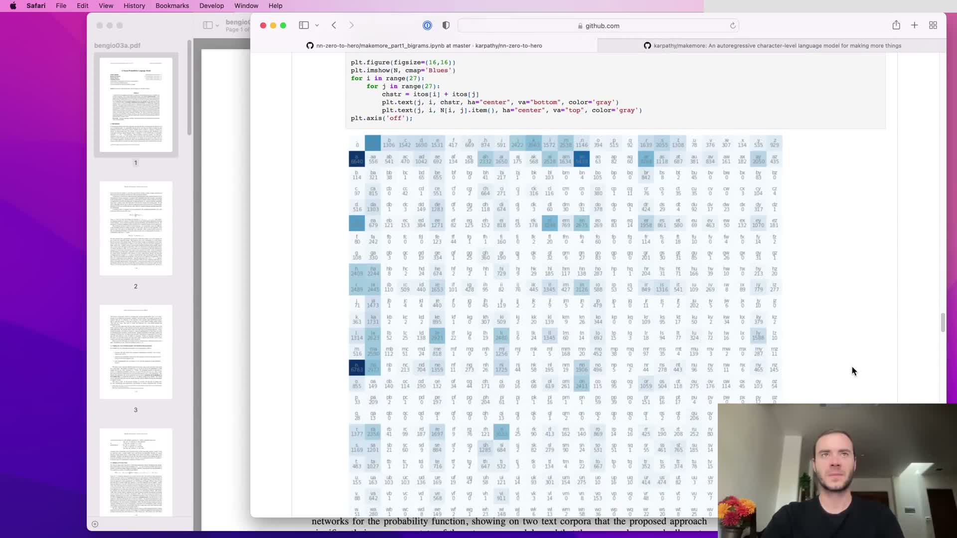
The bigram approach models the next-character probability conditioned only on the immediately preceding character by collecting counts and normalizing rows to probabilities.
This yields a simple 27x27 conditional probability table when using characters: each row sums to one and corresponds to a single previous-character context.
While straightforward and interpretable, relying on a one-character context severely limits the model’s ability to produce realistic sequences because it cannot condition on longer history — motivating models that incorporate longer context without exponential parameter growth.
Context length causes exponential growth in n-gram tables

Extending n-gram counts to longer contexts causes the conditional probability table to grow exponentially with context length:
- 27 possibilities for 1 char
- 27^2 possibilities for 2 chars
- 27^3 possibilities for 3 chars, and so on
This combinatorial explosion produces many context entries with few or zero counts, leading to severe data sparsity and poor generalization.
The inefficiency of large dense count tables motivates using parameter-sharing function approximators that compress context into lower-dimensional representations. Neural network language models learn distributed representations that generalize across similar contexts rather than enumerating every context tuple.
Adopt a multilayer perceptron language model following Bengio et al. 2003

The proposed approach is a feedforward neural network that predicts the next token from a fixed window of previous tokens, following Bengio et al. (2003).
Key components:
- Each context token is mapped to a learned low-dimensional embedding vector.
- Context embeddings are concatenated, passed through one or more fully connected hidden layers with nonlinearities, and finally projected to a vocabulary-sized output layer.
- Training maximizes log-likelihood (equivalently minimizes cross-entropy), and all parameters — embeddings, hidden weights, and output weights — are learned by backpropagation.
This architecture enables parameter sharing and generalization across contexts that share similar constituent tokens.
Token embeddings: low-dimensional learned representations for vocabulary items
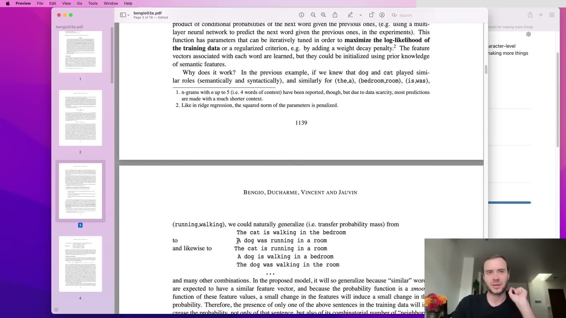
Each vocabulary item (words originally, or characters here) is associated with a learned d-dimensional feature vector.
- The lookup table C is a V x d matrix, where V is vocabulary size.
- Embeddings are initialized randomly and then tuned by gradient-based optimization so semantically or syntactically similar tokens occupy nearby locations in embedding space.
- This distributed representation compresses discrete tokens into a continuous space, enabling transfer of statistical strength across similar tokens and alleviating data sparsity in unseen combinations.
Embeddings form the first layer of the neural language model and are treated as trainable parameters.
Embedding-based generalization enables transfer across unseen n-grams
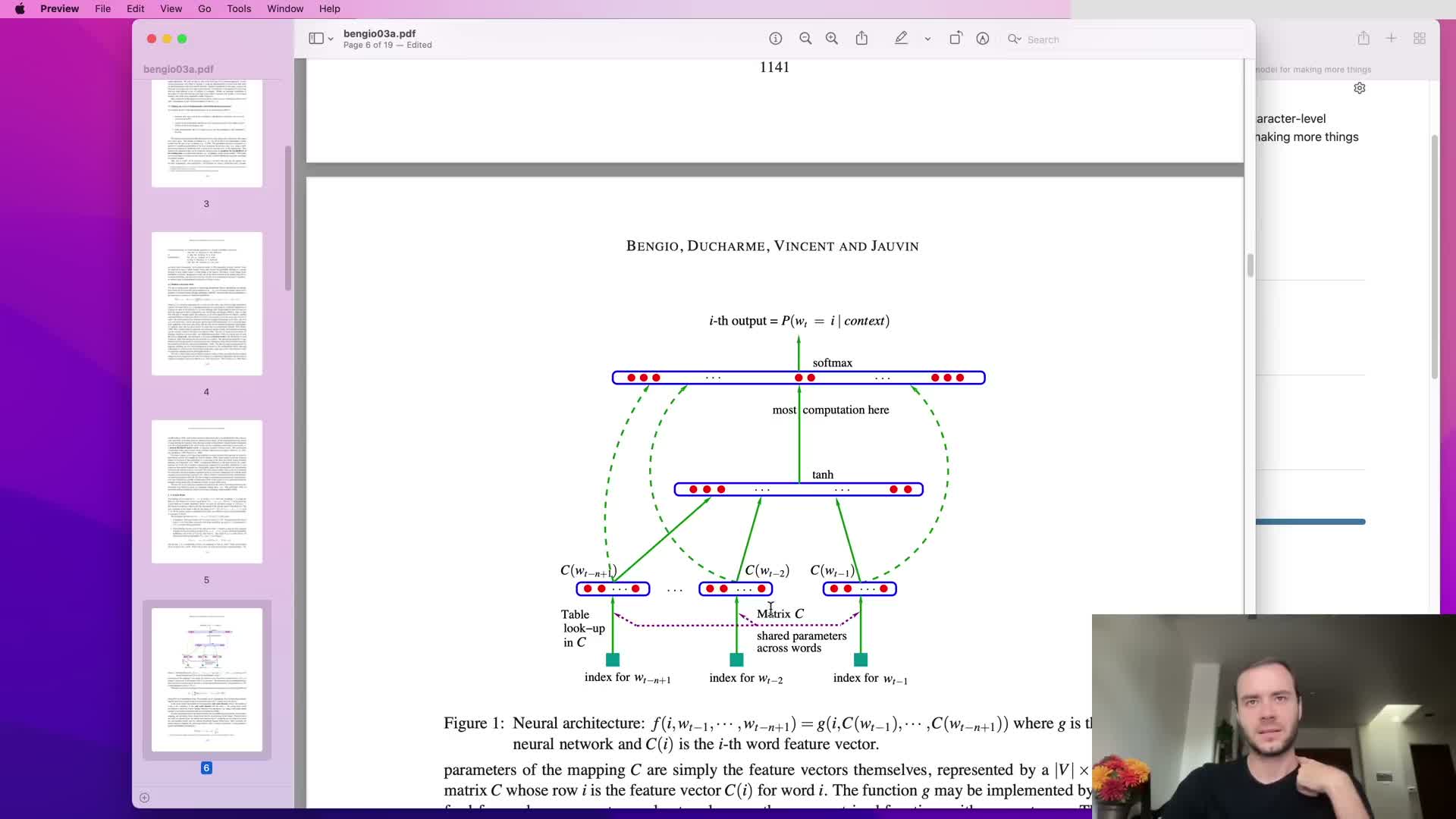
Because tokens are embedded into continuous vectors, the model can generalize to unseen n-grams by leveraging proximity in embedding space.
- Tokens that behave similarly in context (e.g., “a” and “the”, or “cat” and “dog”) will have similar embeddings.
- When the network encounters a novel sequence that shares components with seen sequences, those shared embeddings produce activations that bias predictions toward plausible continuations.
This embedding-driven smoothing distributes probability mass across related contexts in a principled way and is a core reason neural language models outperform raw n-gram estimators on sparse data.
Network architecture: embedding lookup, hidden layer, output softmax

Model forward pass structure:
- Concatenate embeddings of the previous k tokens to form an input vector of size k·d.
- Apply a fully connected hidden layer of size H with a nonlinearity (lecture used tanh).
- Project to a linear output layer producing V logits (V = vocabulary size).
- Convert logits to probabilities via softmax: p = softmax(logits) = exp(logits) / sum exp(logits).
When V is large, the final linear layer contains the majority of parameters and computation, making it the primary computational bottleneck.
Training jointly optimizes embeddings, hidden weights, and output weights to maximize the likelihood of observed next tokens.
Model parameters are optimized end-to-end with backpropagation
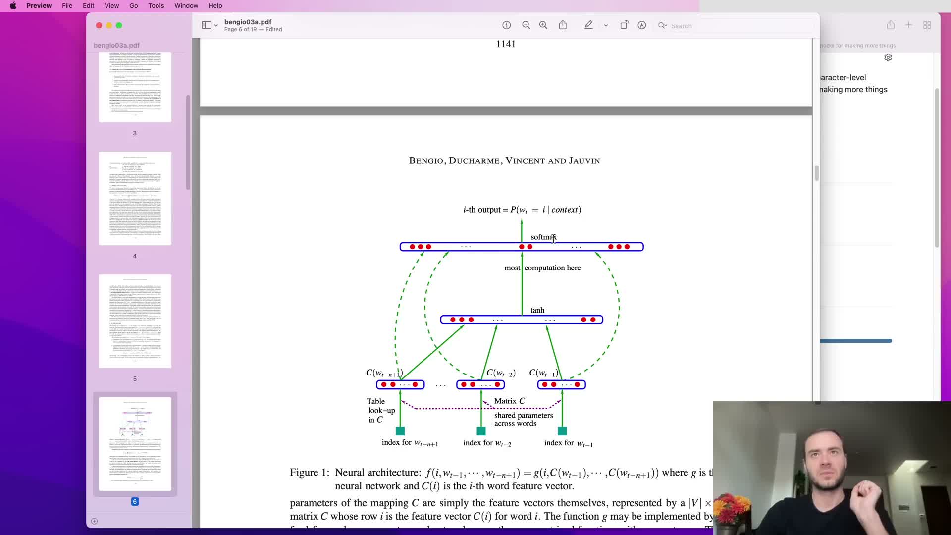
All model parameters — the embedding lookup matrix C, hidden layer weights and biases, and output layer weights and biases — are optimized using gradient-based learning and backpropagation.
Training example procedure:
- Forward pass produces a probability for the true next token.
- Compute cross-entropy loss.
- Backpropagate gradients to accumulate parameter derivatives.
- Update parameters with gradient steps scaled by a learning rate (or using other optimizers).
This end-to-end learning lets embeddings move in the space to improve predictive performance of downstream layers.
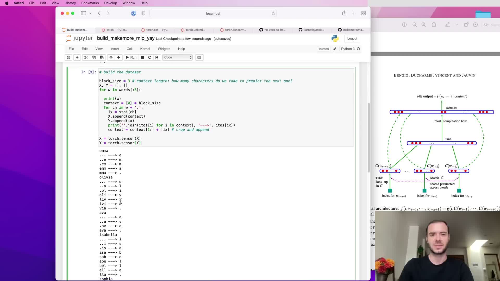
Construct dataset using sliding context windows and block size
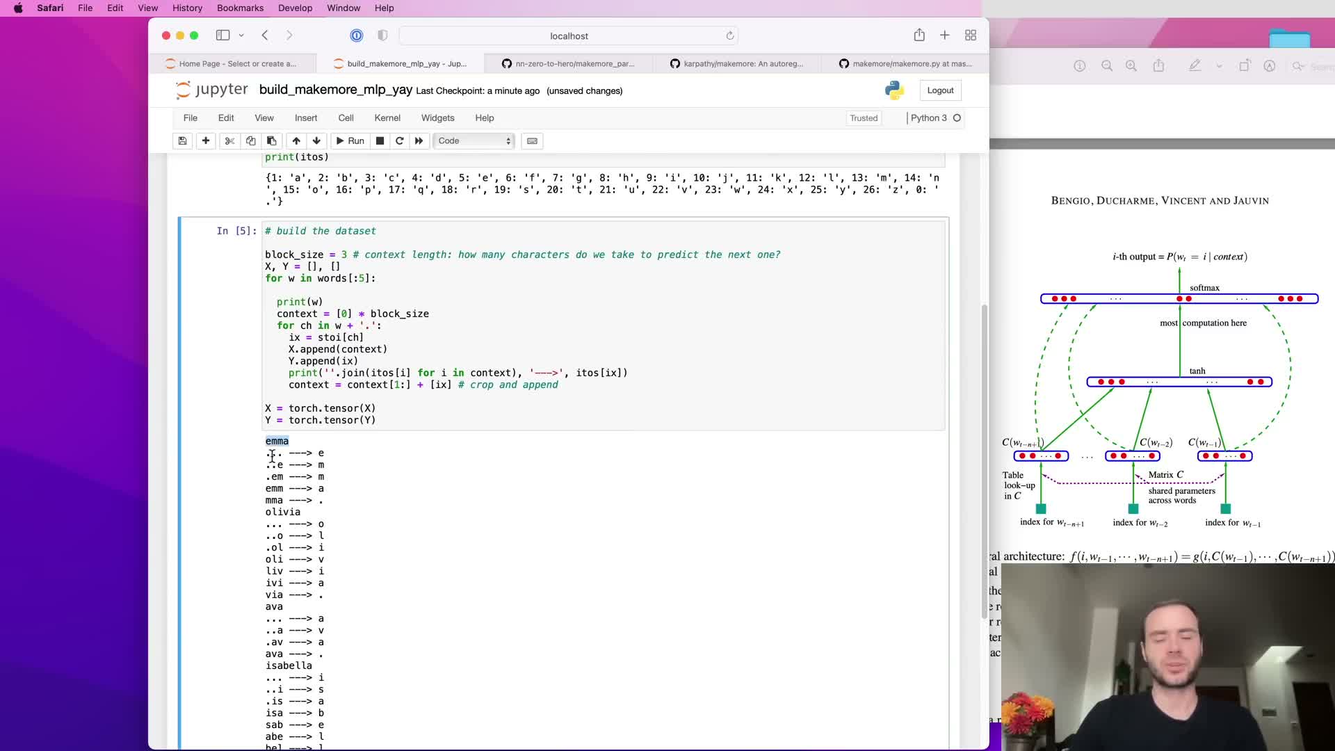
Constructing the dataset uses a sliding fixed-size context window (block size k) across each training string to create input-output pairs:
- Input x is the k previous token indices.
- Label y is the next token index.
- Use padding tokens (dots) to represent positions before the start of the string, enabling learning from prefixes.
Block size controls the model’s receptive field: k=3 uses three previous characters to predict the fourth; larger k increases context but also increases dimensionality of concatenated embeddings.
This windowing converts raw token sequences into a large supervised training set suitable for batch training.
Embedding lookup vs one-hot multiplication: equivalence and dtype care
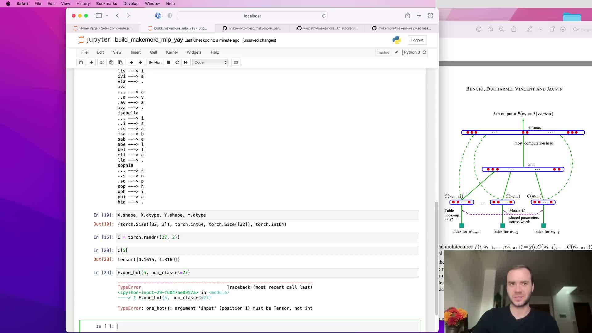
An embedding lookup that retrieves row i of C is mathematically equivalent to multiplying a one-hot vector for index i by the embedding matrix C (the one-hot masks all rows except the i-th).
Practically, direct integer indexing into C is far more efficient than constructing one-hot vectors and performing a matrix multiply.
Care points:
- One-hot encodings produced as integer tensors must be cast to floating types before multiplying by floating-point embedding matrices.
- Using direct indexing avoids unnecessary intermediate tensors and yields both speed and memory benefits.
Batch embedding via advanced indexing: embedding entire x tensor at once
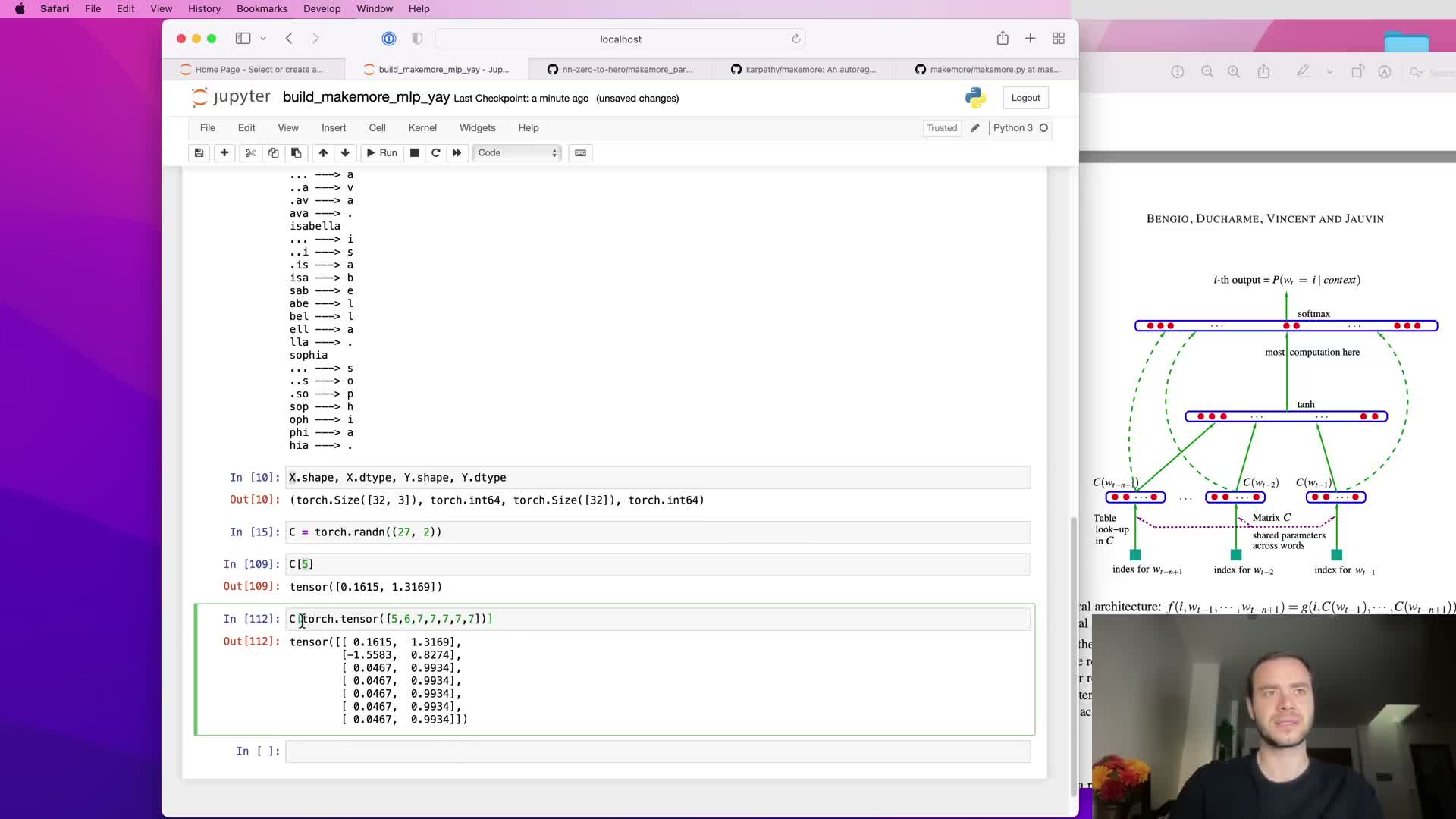
Modern tensor libraries allow indexing a matrix C with a multi-dimensional integer tensor X of shape (B, k) to produce an embedded tensor of shape (B, k, d) in a single operation.
- This pulls appropriate row vectors for all examples and context positions simultaneously.
- It enables efficient vectorized computation for an entire mini-batch and avoids Python loops.
- The result exploits optimized C/CUDA kernels and is ready for subsequent reshaping and linear operations.
Concatenation and reshaping: preparing embeddings for a linear hidden layer
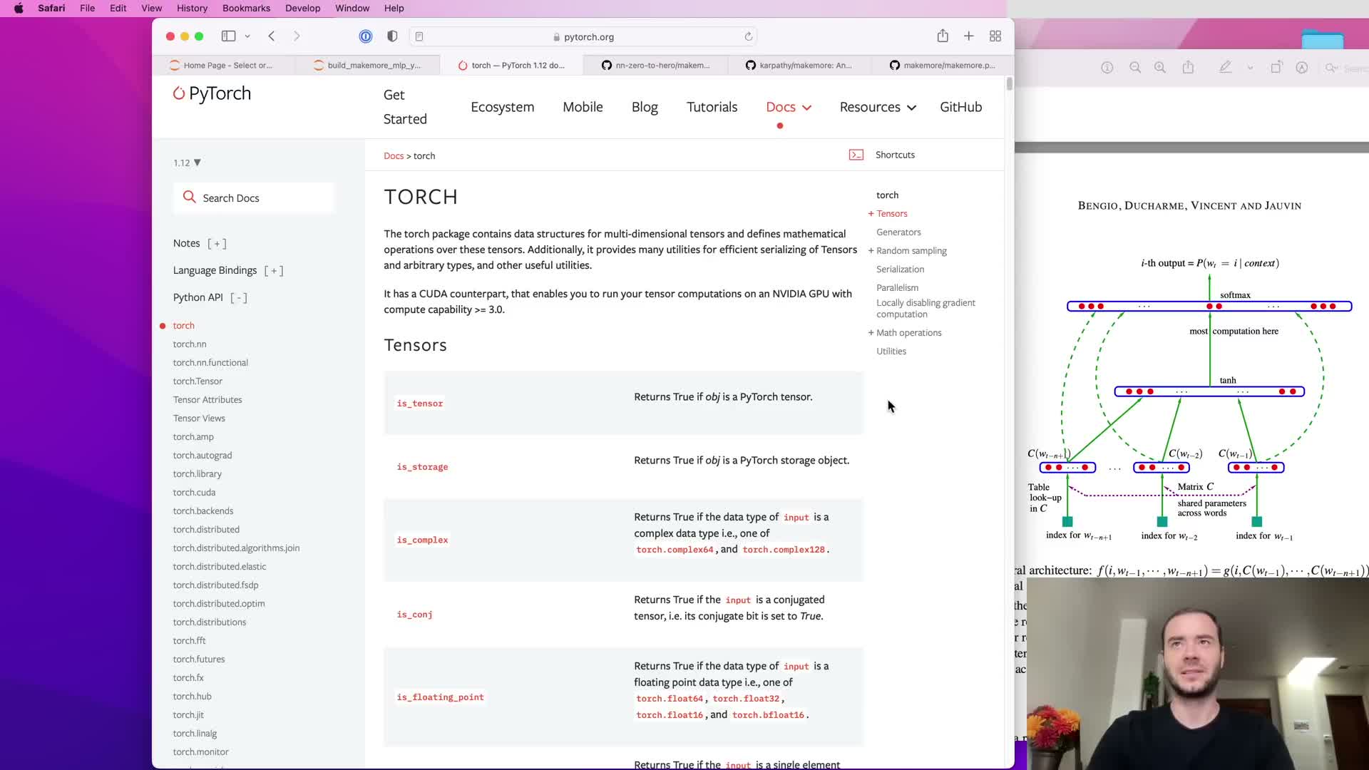
To feed concatenated embeddings into a fully connected hidden layer, reshape the (B, k, d) tensor to (B, k·d) so each example becomes a single flat input vector.
- Naive concatenation with cat creates new tensors and extra memory allocation.
- A more efficient approach is to use view/reshape to reinterpret the same underlying storage as (B, k·d), incurring no data copy when the layout is compatible.
Correct reshaping ensures the input matrix multiplies cleanly with the hidden weight matrix of shape (k·d, H) to produce (B, H) pre-activations.
use of unbind and cat for generic concatenation across variable block size
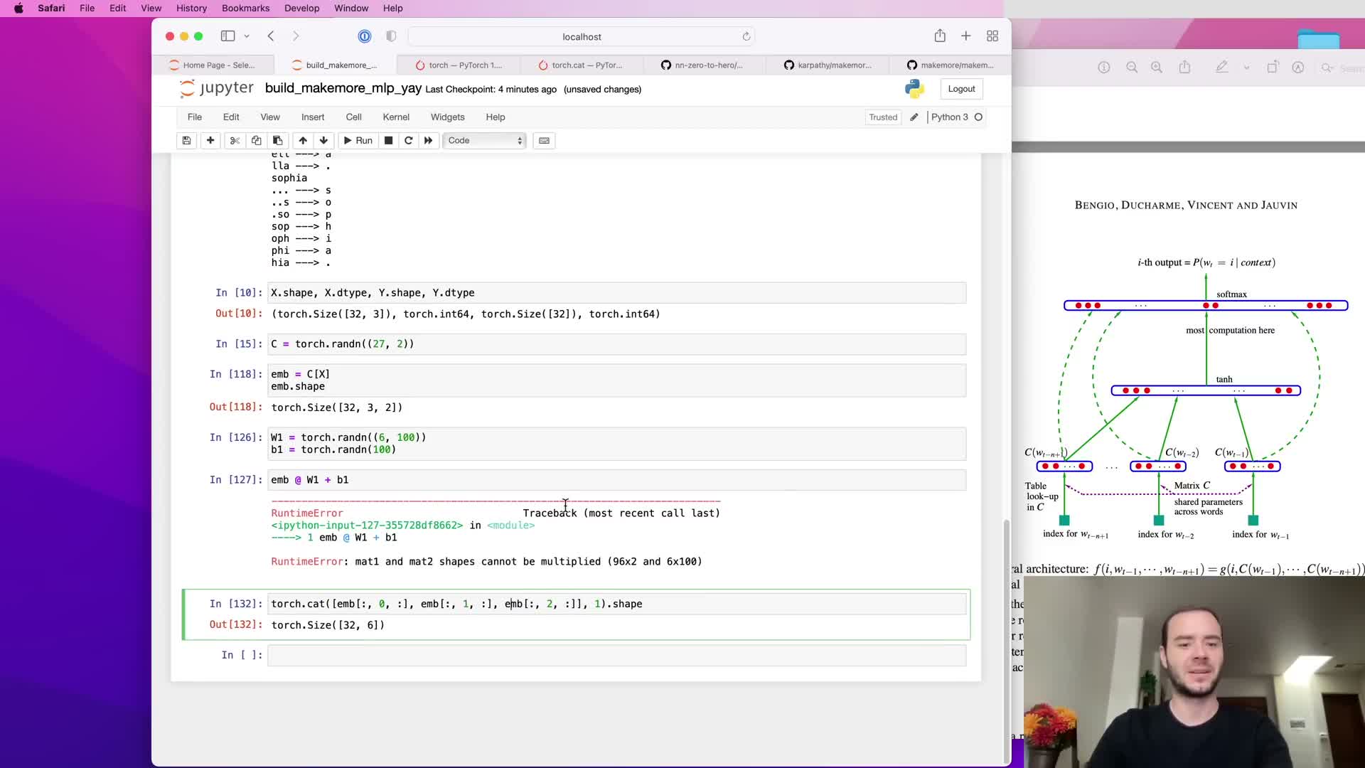
When block size k is not known at code-writing time, tensor libraries provide utilities such as unbind to split a tensor into a tuple of k slices; these slices can then be concatenated with cat along the embedding axis.
- Calling torch.unbind(X, dim=1) yields an iterable of tensors for each context position.
- torch.cat applied along the feature dimension constructs flattened inputs and generalizes to arbitrary k.
Trade-off: unbind+cat is readable and flexible but may allocate new memory; prefer view/reshape for maximum efficiency when data layout already matches the flattened layout.
Tensor view/reshape and underlying storage enable zero-copy reinterpreting
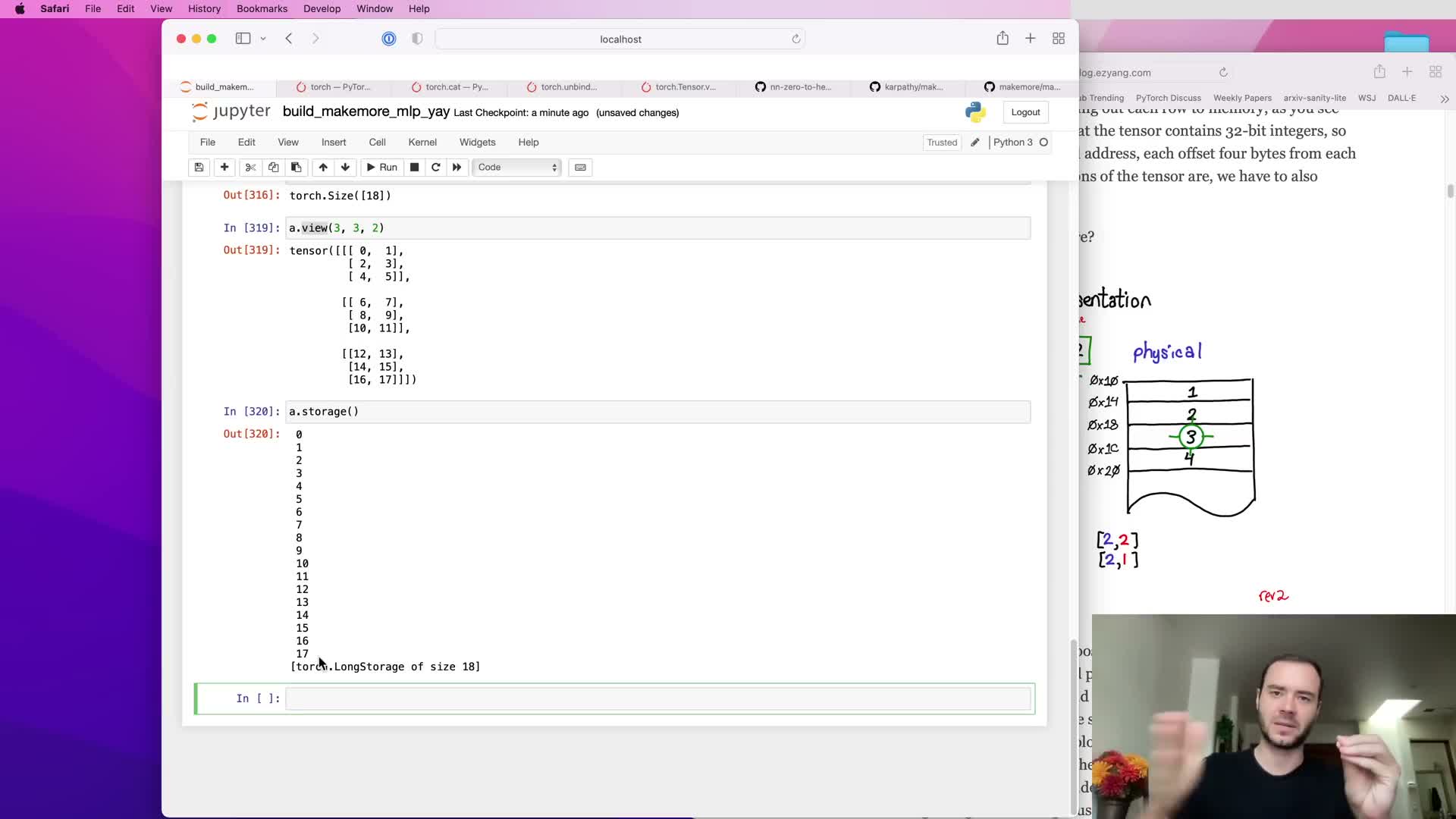
A view (reshape) operation reinterprets the same one-dimensional underlying storage with different strides and shape metadata without copying data.
- Tensors have an underlying storage buffer; view manipulates metadata such as storage offset, shape, and strides to present an n-dimensional array from the same memory.
- Because view is a no-copy operation, it is extremely efficient for flattening (B, k, d) to (B, k·d) when data layout is compatible.
Understanding storage and stride semantics is important to avoid unexpected copies and to write high-performance tensor code.
Hidden layer computation, nonlinearity, and broadcasting of biases
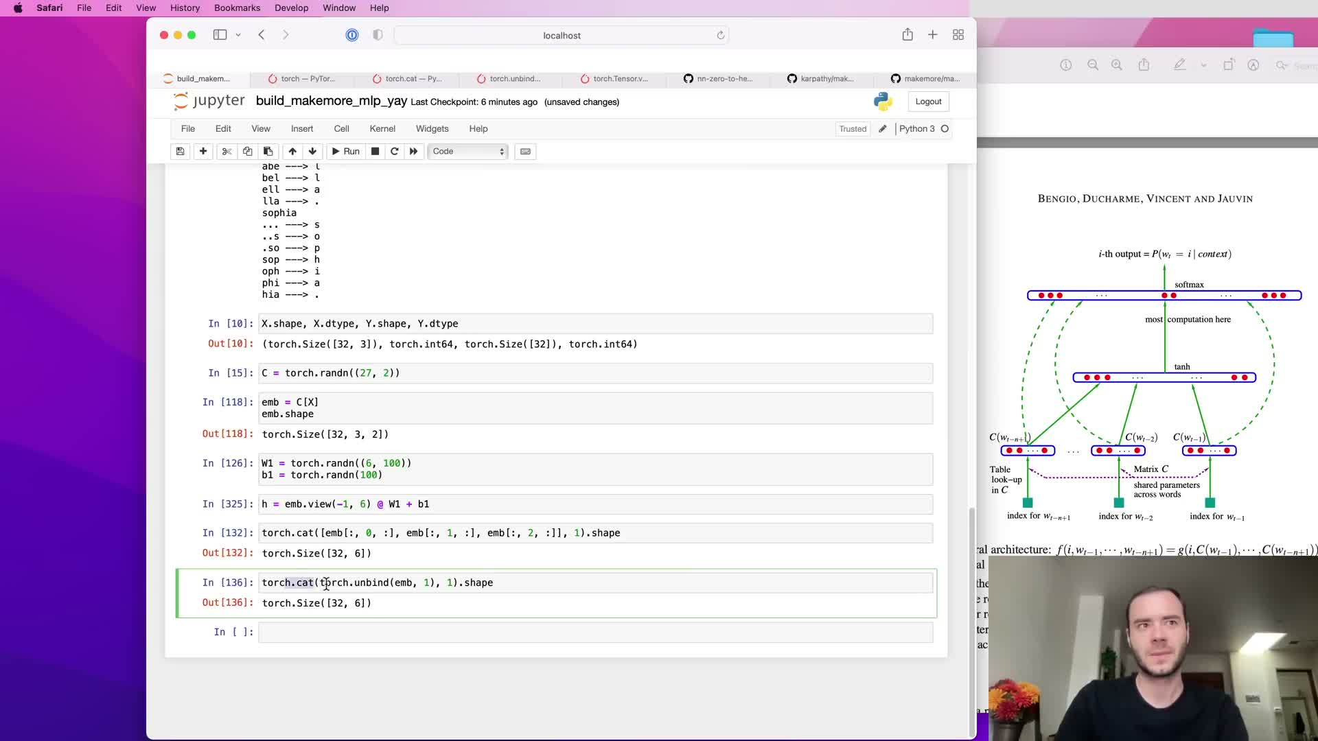
After reshaping to (B, k·d), compute hidden pre-activations as:
-
h_pre = X_flat @ W1 + b1, where W1 is (k·d, H) and b1 is length H.
- Apply a nonlinearity (e.g., tanh) element-wise to produce hidden activations h = tanh(h_pre). tanh bounds activations to (-1, 1) and introduces nonlinearity for representation learning.
When adding bias b1 to the (B, H) pre-activation matrix, broadcasting expands b1 to (B, H) so the same bias is added to every example; correct shape alignment and broadcasting semantics ensure intended parameter sharing across the batch.
Final linear layer, softmax, and negative log-likelihood loss
The hidden activations h of shape (B, H) are multiplied by the output weight matrix W2 of shape (H, V) and added to bias b2 to produce logits of shape (B, V).
- The softmax function converts logits to a per-example probability distribution: p = softmax(logits).
- Given true target indices y of length B, the negative log-likelihood (cross-entropy) loss is computed as L = -mean(log p[i, y[i]]) and serves as the scalar objective minimized during training.
Proper numerical handling of softmax and log operations is important to avoid overflow and underflow.
use of torch.nn.functional.cross_entropy for efficiency and numerical stability
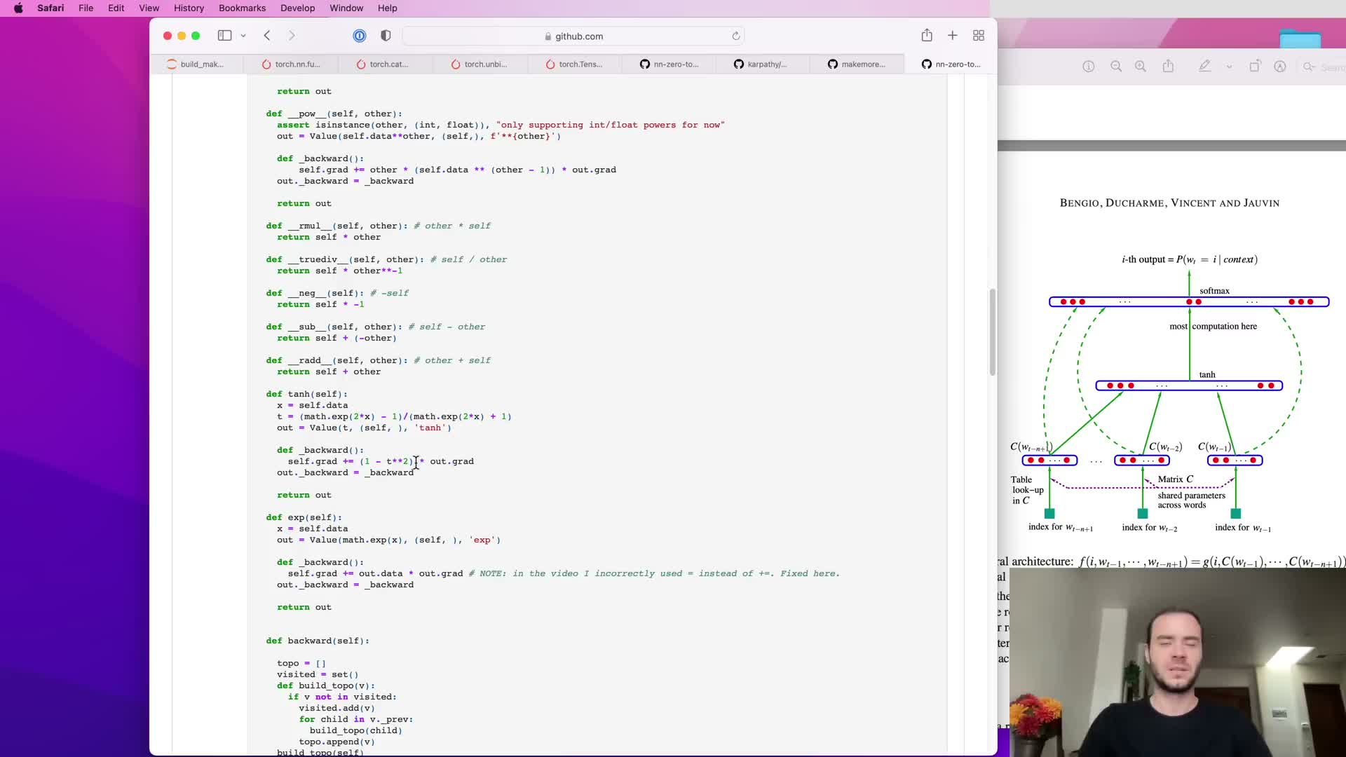
Instead of explicitly exponentiating logits and normalizing to compute cross-entropy, use the framework’s fused cross-entropy routine, which implements softmax + log + negative-log-likelihood in a numerically stable and efficient kernel.
Benefits:
- Avoids creating large transient tensors and enables kernel fusion for forward computation.
- Often provides a mathematically simplified and cheaper backward pass.
- Implements the log-sum-exp trick (subtracting the maximum logit per row) to prevent overflow when logits are large.
Using the framework’s cross-entropy routine is recommended for both correctness and performance.
Training loop mechanics: zeroing gradients, backward pass, and parameter update
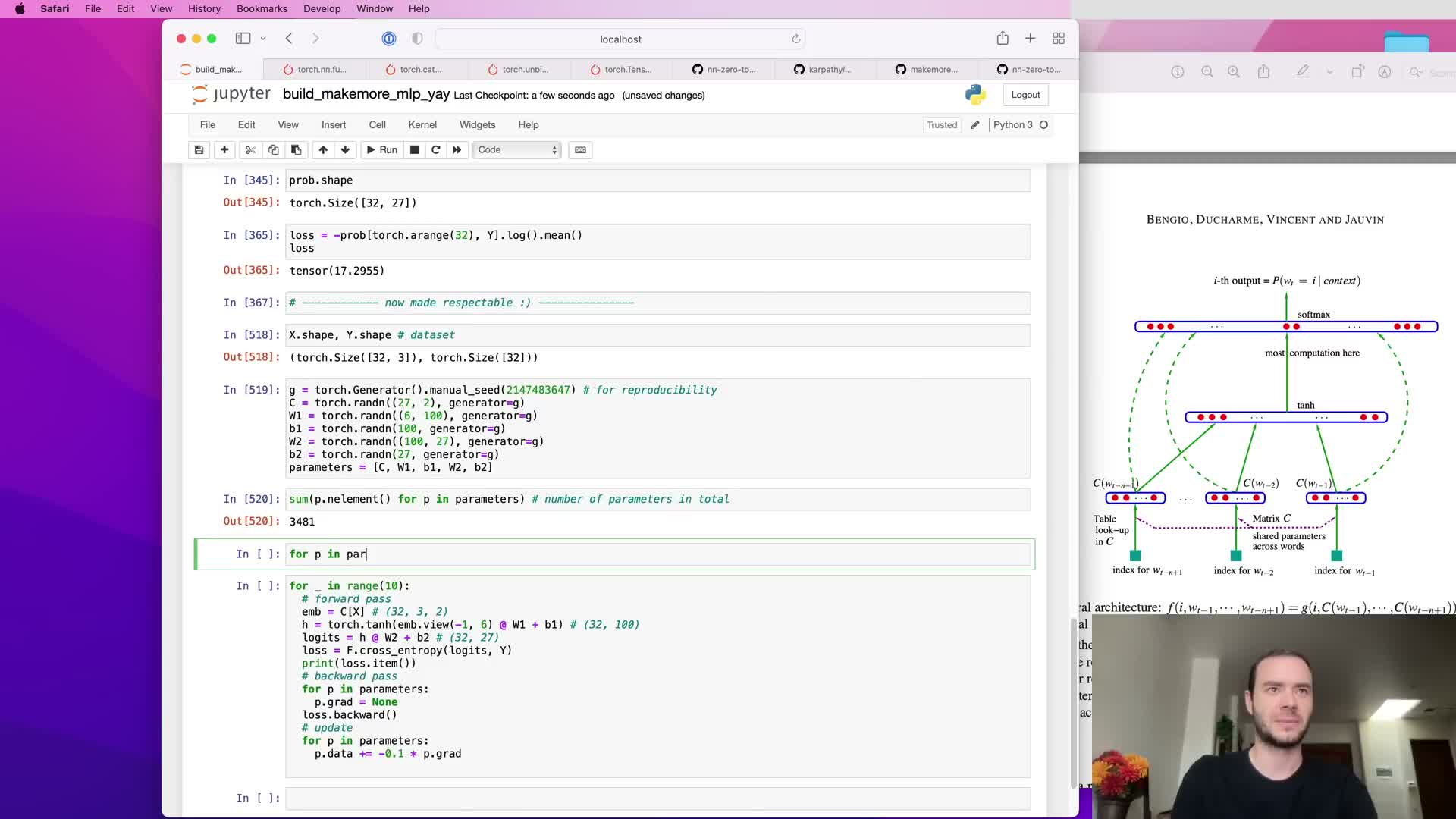
A basic training iteration consists of:
- Zeroing/resetting gradients for all parameters.
- Performing a forward pass to compute the loss.
- Calling backward on the loss to accumulate gradients.
- Updating parameters (e.g., p -= lr * p.grad for simple SGD).
Implementation notes:
- All parameter tensors must have requires_grad=True for autograd to track operations and populate gradients.
- Repeat the loop for many iterations to decrease training loss, but be mindful of overfitting on small datasets or oversized models.
Proper batching, learning rate selection, and regularization are necessary to obtain models that generalize.
Mini-batch stochastic gradient descent: sampling indices and reducing computation
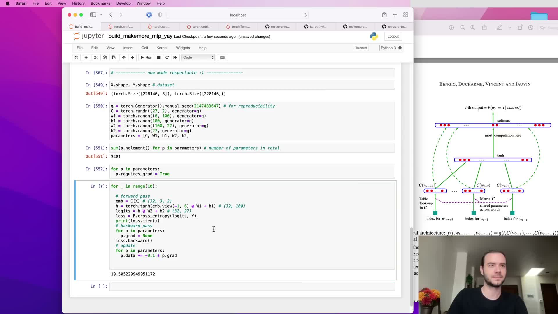
Processing the entire dataset for every gradient update is costly; instead, draw random mini-batches of example indices and compute forward/backward passes on those subsets.
- Generate a random integer index tensor ix of shape (B,) and index X[ix] and y[ix] to yield a batch.
- Complexity for the batch is proportional to B, not the entire dataset.
Mini-batch SGD trades exact gradient direction for a noisy but efficient estimate, allowing many more parameter updates per unit time and faster empirical convergence. Batch size is a tunable trade-off between gradient variance, throughput, and generalization behavior.
Learning rate selection with an exponential sweep (LR finder)
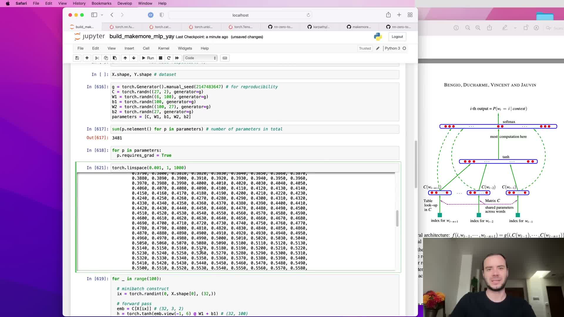
A systematic way to choose a learning rate is an LR sweep:
- Initialize parameters.
- Run a short optimization loop while exponentially increasing the learning rate across a range (e.g., 10^{-3} to 10^{0}).
- Record loss as a function of learning rate (or exponent).
- Plot loss vs. learning rate and pick the value in the valley before loss explodes.
Practically, create a sequence of exponents linearly spaced and set lr = 10^{lre[i]} during iteration i. This empirical method gives a practical starting point for longer training schedules.
Train/validation/test splits and roles of each split
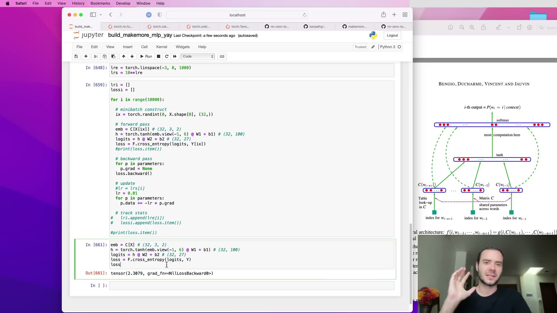
Proper model evaluation requires splitting data into training, development (dev), and test sets (common splits: 80%/10%/10%) to separate parameter optimization from hyperparameter selection and final assessment.
- Training split: used for gradient-based parameter optimization.
- Dev split: used to tune hyperparameters (hidden size, embedding dimension, batch size, learning rate schedules, regularization).
- Test split: held out for final evaluation and reported performance; use sparingly after hyperparameters are fixed to avoid information leakage.
Monitoring dev loss versus training loss helps diagnose underfitting vs. overfitting.
Functionized dataset construction, shuffling, and split sizes
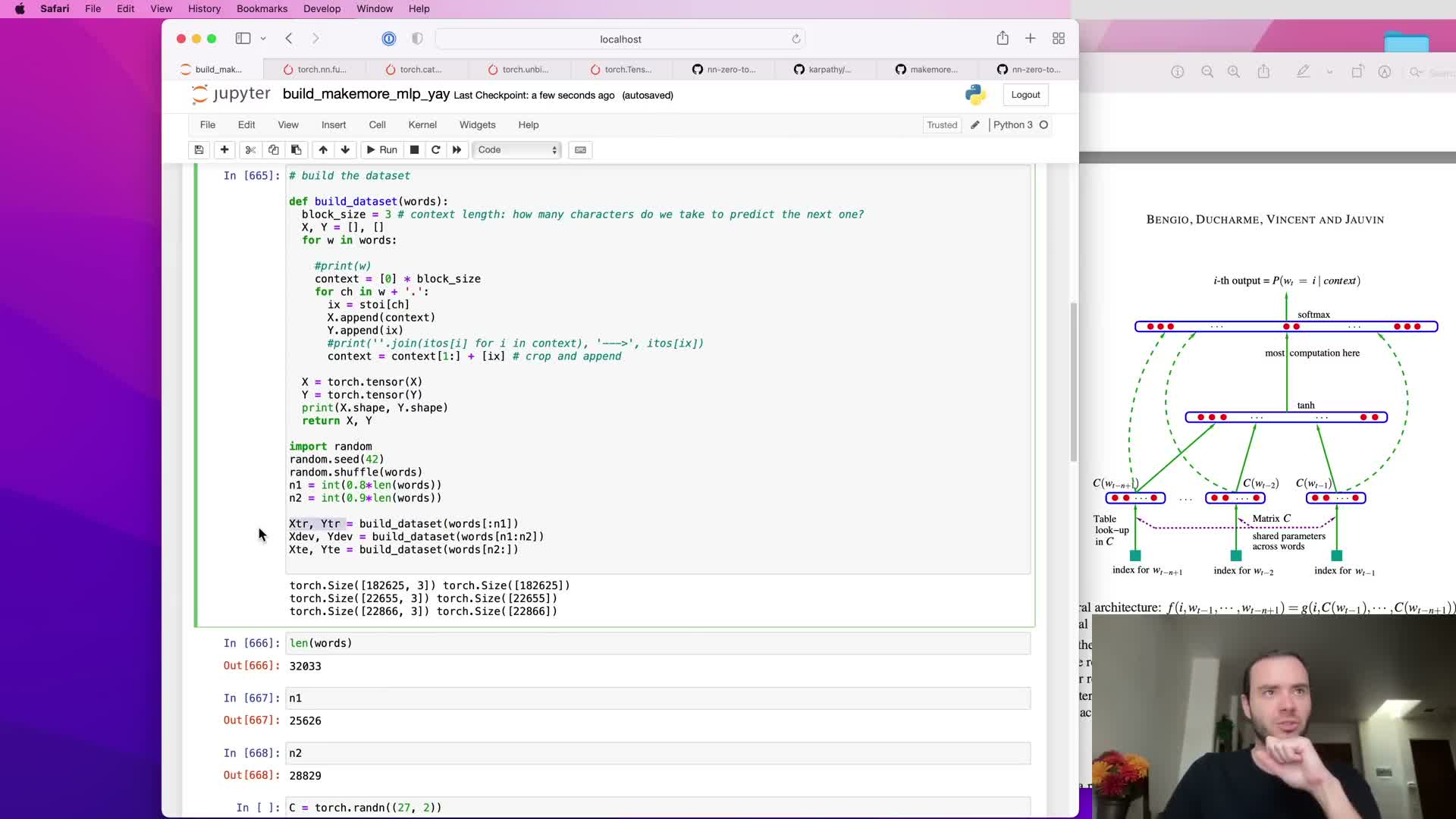
Encapsulating dataset-building logic into a function simplifies experiments:
- The function can create X and y tensors for arbitrary word/character lists while shuffling inputs to remove ordering biases.
- It can compute split indices n1 and n2 to partition training/dev/test sets deterministically or randomly.
- For large corpora this produces training sets on the order of tens of thousands of examples and smaller dev/test subsets for development.
Encapsulation makes it easy to vary block size, vocabulary, or dataset subsets without rewriting low-level data-processing code.
Scaling model capacity: hidden layer increase and underfitting diagnosis
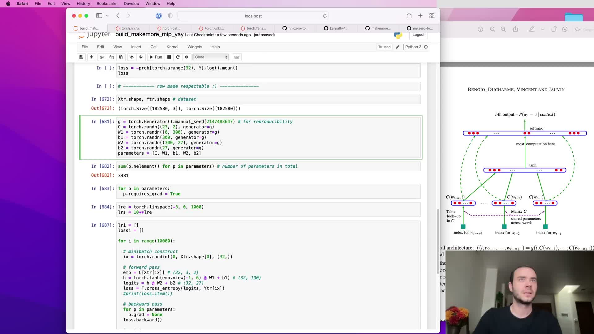
Increasing hidden layer size raises model capacity and parameter count.
- If training and dev losses are roughly equal and both high, the model is underfitting and more capacity or representational changes are likely beneficial.
- Scaling hidden units (e.g., from 100 to 300) increases parameter count and flexibility but requires more careful tuning of learning rates and batch sizes to avoid noisy optimization.
Observe training and dev curves to decide whether to increase capacity, change embeddings, or alter optimization hyperparameters.
Visualizing 2D character embeddings reveals learned structure
When embedding dimension d is small (e.g., d = 2), learned embeddings can be visualized in the plane by plotting the two coordinates for each token and annotating with token labels.
- Visualization often reveals clustering by functional or distributional similarity (e.g., vowels cluster, punctuation and rare letters occupy separate regions, outliers like ‘q’ may appear isolated).
- Such plots provide qualitative insight into token similarity and can indicate whether embedding capacity is a bottleneck.
Visualization is useful during development but becomes infeasible when d > 3.
Increase embedding dimensionality and further training to reduce loss
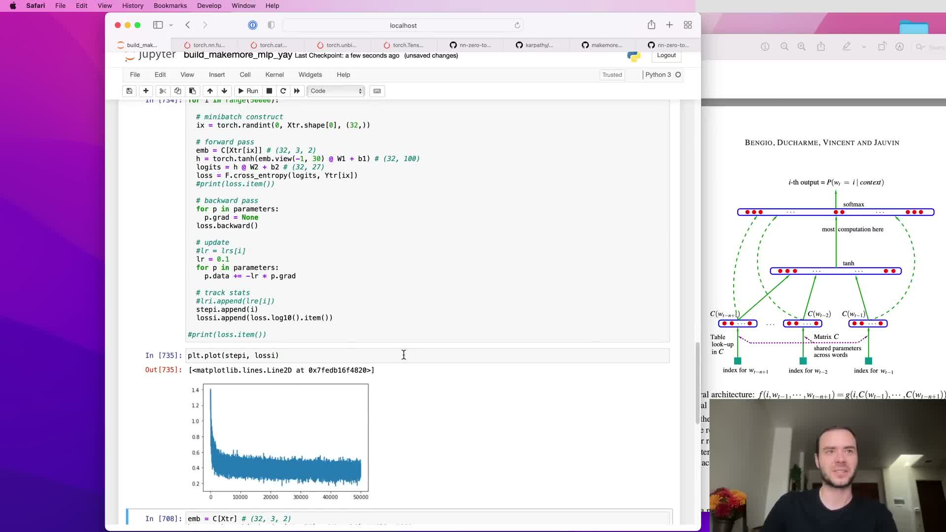
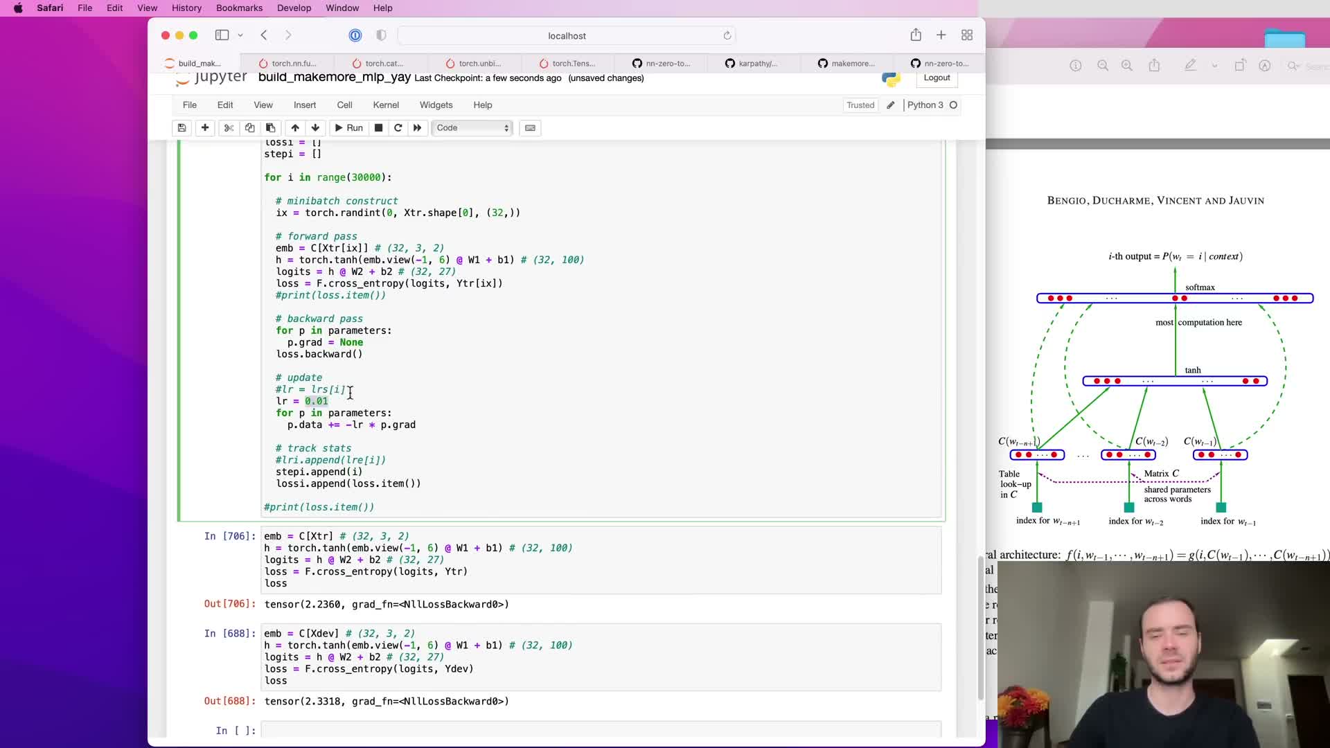
If the model underfits even after increasing hidden capacity, expanding embedding dimensionality (e.g., from d=2 to d=10) increases representational capacity and changes input size to the hidden layer from k·d_old to k·d_new.
- Adjust hidden layer size accordingly and retrain with an appropriate learning rate schedule (including staged decay).
- Empirically tune batch size, number of training steps, learning rate, and decay schedule; the lecture reports a best validation loss around 2.17 with careful experimentation.
Hyperparameter search over embedding size, context length, hidden size, and optimization schedule is the standard route to further improvements.
Sampling from the trained model using autoregressive generation
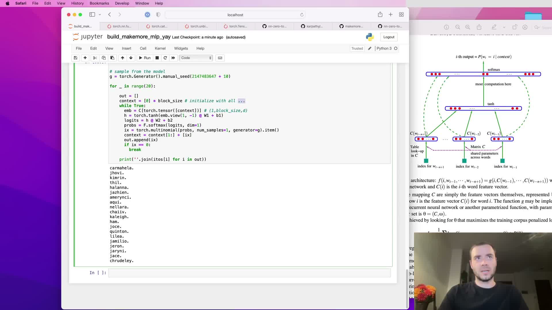
Autoregressive sampling generates sequences by repeatedly predicting the next token conditioned on the current k-length context:
- Embed the current context (k tokens).
- Compute logits and convert to softmax probabilities (use a numerically stable softmax).
- Draw the next token index via multinomial sampling from the distribution.
- Append the sampled token to the context and repeat until a termination condition.
For single-example generation use batch dimension 1. Stochastic sampling from the learned distribution produces novel outputs that reflect model generalization — with a trained MLP over characters the outputs become more name-like compared to a bigram baseline. Sampling is useful for qualitative assessment of learned sequence structure and creativity.
Provision of executable Colab notebooks to reproduce and tinker
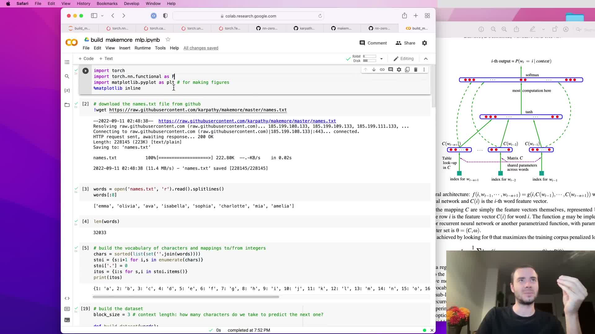
Providing a hosted Google Colab notebook enables reproducible execution of data preprocessing, model construction, training, plotting, and sampling without local installation of Jupyter or deep learning frameworks.
- The notebook mirrors implementation steps and allows hyperparameter modification in-browser.
- It lowers the barrier for reproducing results, exploring alternative architectures, and performing hyperparameter sweeps.
Colab is recommended for hands-on replication and extension of the model and experiments described.
Enjoy Reading This Article?
Here are some more articles you might like to read next: