Karpathy Series - Bulding Makemore Part 3 - Activations, Gradients, BatchNorm
- Lecture objectives and importance of activations and gradients
- Starting code and dataset organization for the MLP implementation
- Use of no-grad context for efficient evaluation and sampling procedure
- Symmetry and expected initial loss at the softmax output
- Output-layer initialization: bias and weight scaling to avoid overconfident logits
- Training dynamics after fixing output-layer scaling (hockey-stick effect)
- Tanh hidden-layer saturation and its impact on gradients
- Dead neurons and nonlinearity-specific failure modes
- Mitigating hidden-unit saturation by scaling weights and biases
- Empirical demonstration of initialization improvements on validation loss
- Principled variance preservation via fan-in scaling (Xavier/Kaiming motivation)
- Adjusting initialization gains for nonlinearities and He/Kaiming initialization
- Modern mitigations that relax fragile initialization requirements
- Batch normalization: standardizing activations per batch to control statistics
- Learned scale and shift (gamma and beta) and avoiding permanent Gaussian forcing
- BatchNorm inference: calibration, running statistics, and no-grad updates
- Numerical safeguards, parameter/buffer semantics and bias handling with BatchNorm
- ResNet design pattern and typical placement of BatchNorm
- PyTorch layer conventions and default initialization behavior
- Need for diagnostics and overview of pyTorch-like modularization
- Practical diagnostics: activation histograms, saturation metrics, gradient histograms, and parameter statistics
Lecture objectives and importance of activations and gradients

The lecture frames the objective as developing an intuitive and diagnostic understanding of neural network activations and backward-flowing gradients because that understanding determines optimization difficulty and explains historical architecture choices (e.g., recurrent networks).
The scope prioritizes mastering how activations and gradients behave during training before moving from a simple multilayer perceptron (MLP) to more complex architectures.
Emphasis is placed on first-order optimization methods and on why certain architectures are harder to optimize, which motivates later discussion of initialization, normalization techniques, and diagnostic tooling used during training.
This conceptual framing establishes why subsequent implementation and analysis details matter for practical model development — it connects low-level behavior (activations/gradients) to high-level design and engineering choices.
Starting code and dataset organization for the MLP implementation
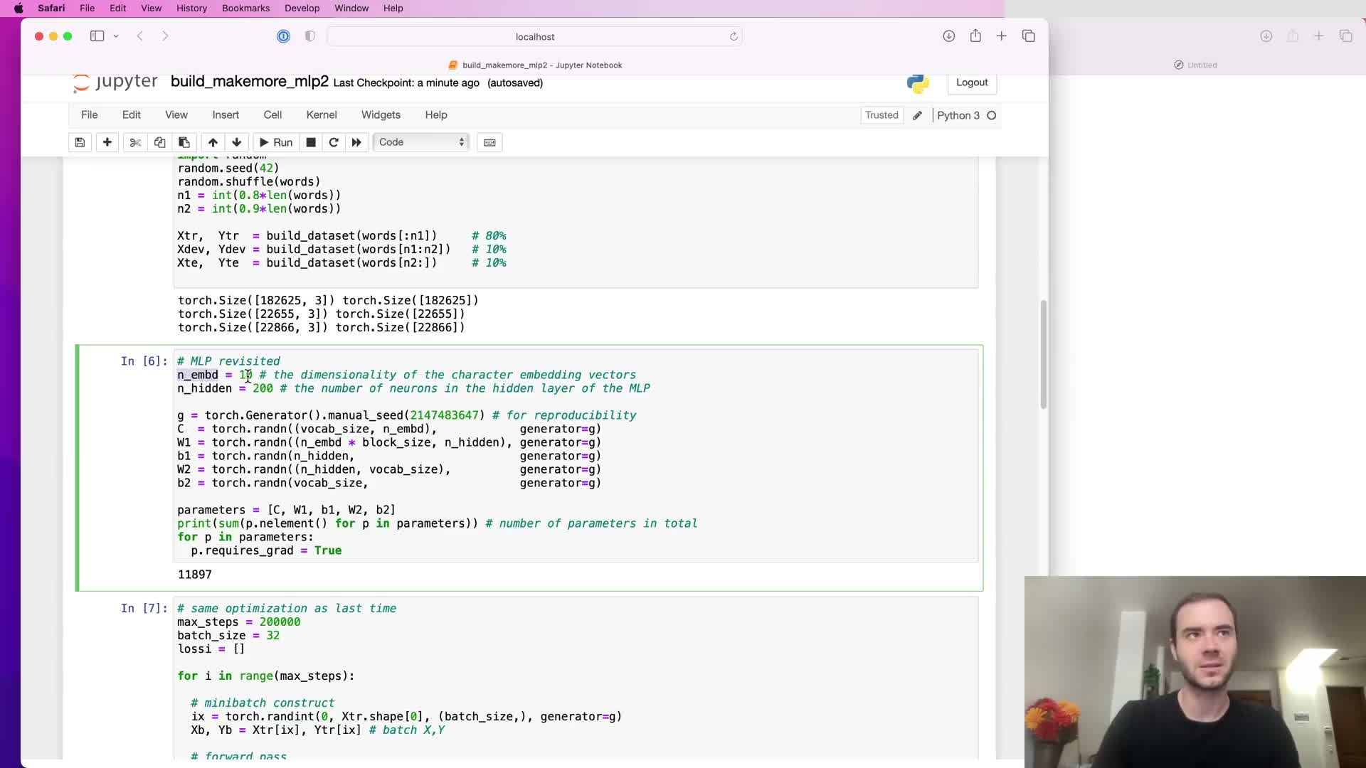
The project uses a character-level language modeling setup with an embedding layer and a multilayer perceptron.
Key dataset and model details:
- Dataset: ~32k training examples with a restricted vocabulary of lowercase letters plus a dot token.
- Architecture: embedding → MLP → softmax over 27 tokens.
- Hyperparameters: embedding dimensionality, number of hidden units, etc., are exposed as named variables (no magic numbers).
- Training regimen: batch size 32 and many optimization steps; evaluation accepts arbitrary splits (train/val/test).
Refactoring and modular organization:
- Exposes hyperparameters for easy experimentation.
- Simplifies swapping architectures, tuning hyperparameters, and adding diagnostics.
- Mirrors common PyTorch code structure for reproducibility and clarity.
Use of no-grad context for efficient evaluation and sampling procedure
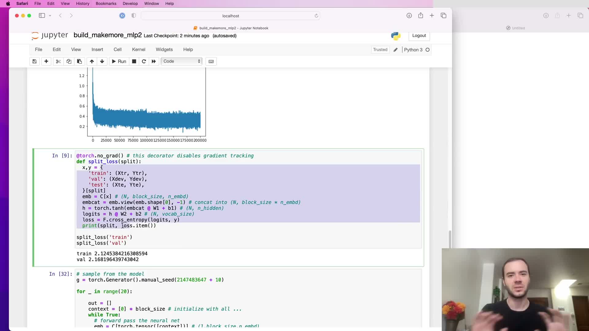
Evaluation code runs inside a no-gradient context (e.g., torch.no_grad decorator or context manager) so validation and sampling forward passes do not build or retain autograd graphs.
Benefits of no-gradient evaluation:
- Reduces memory overhead.
- Reduces compute overhead.
- Ensures correct gradient bookkeeping (no accidental gradient accumulation during evaluation).
The model sampling routine follows the standard autoregressive pattern:
- Use the network to compute output logits and convert them to a probability distribution (softmax).
- Sample a token from that distribution.
- Append the sampled token to the context window and repeat until a termination token is produced.
This separation between training (requires gradients) and evaluation/sampling (no gradients) ensures both efficiency and correctness.
Symmetry and expected initial loss at the softmax output
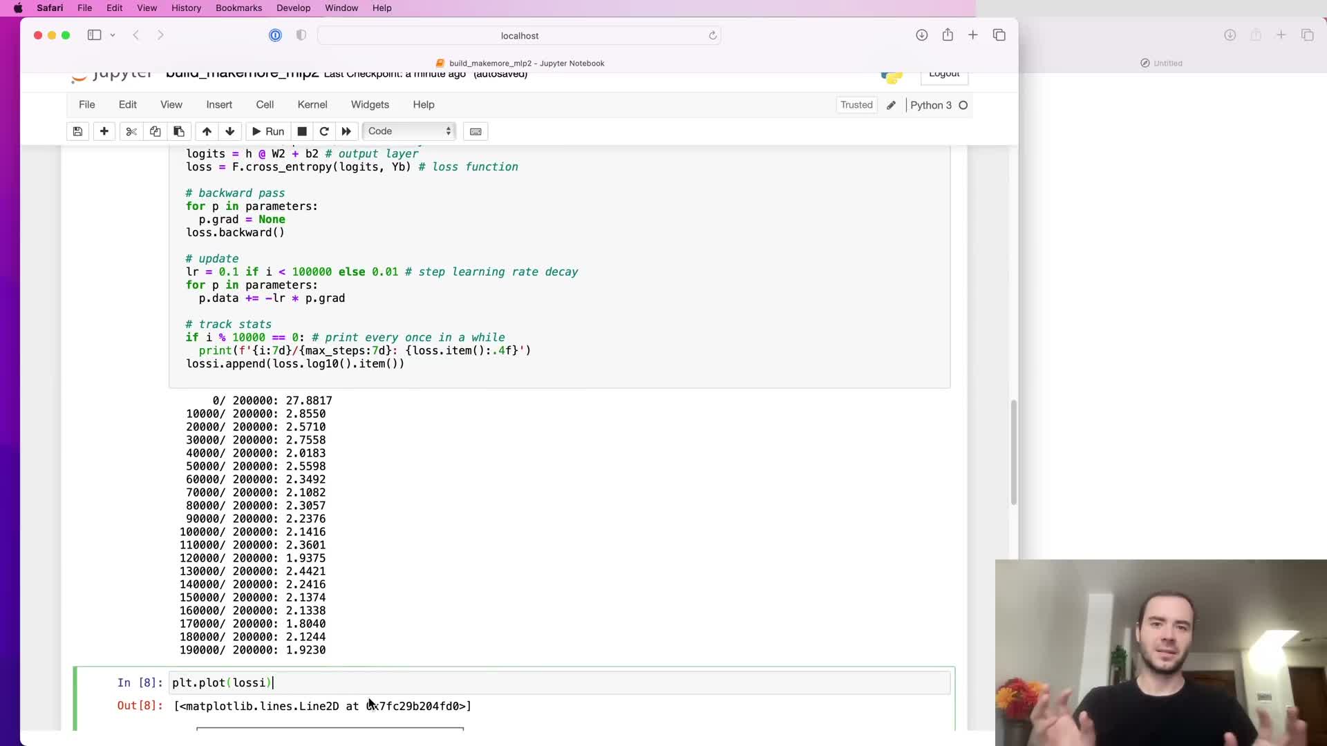
At random initialization the expected predictive distribution should be near-uniform across the 27-character vocabulary, yielding an expected negative log-likelihood of approximately -log(1/27) ≃ 3.29.
If logits at initialization take large, asymmetric values then the softmax can be confidently wrong and produce extremely high loss values — a symptom of poor output-layer initialization.
Therefore, the output layer should be initialized so logits are numerically small and approximately equal across classes to reflect symmetry and avoid wasteful early training that only corrects gross confidence errors.
Output-layer initialization: bias and weight scaling to avoid overconfident logits
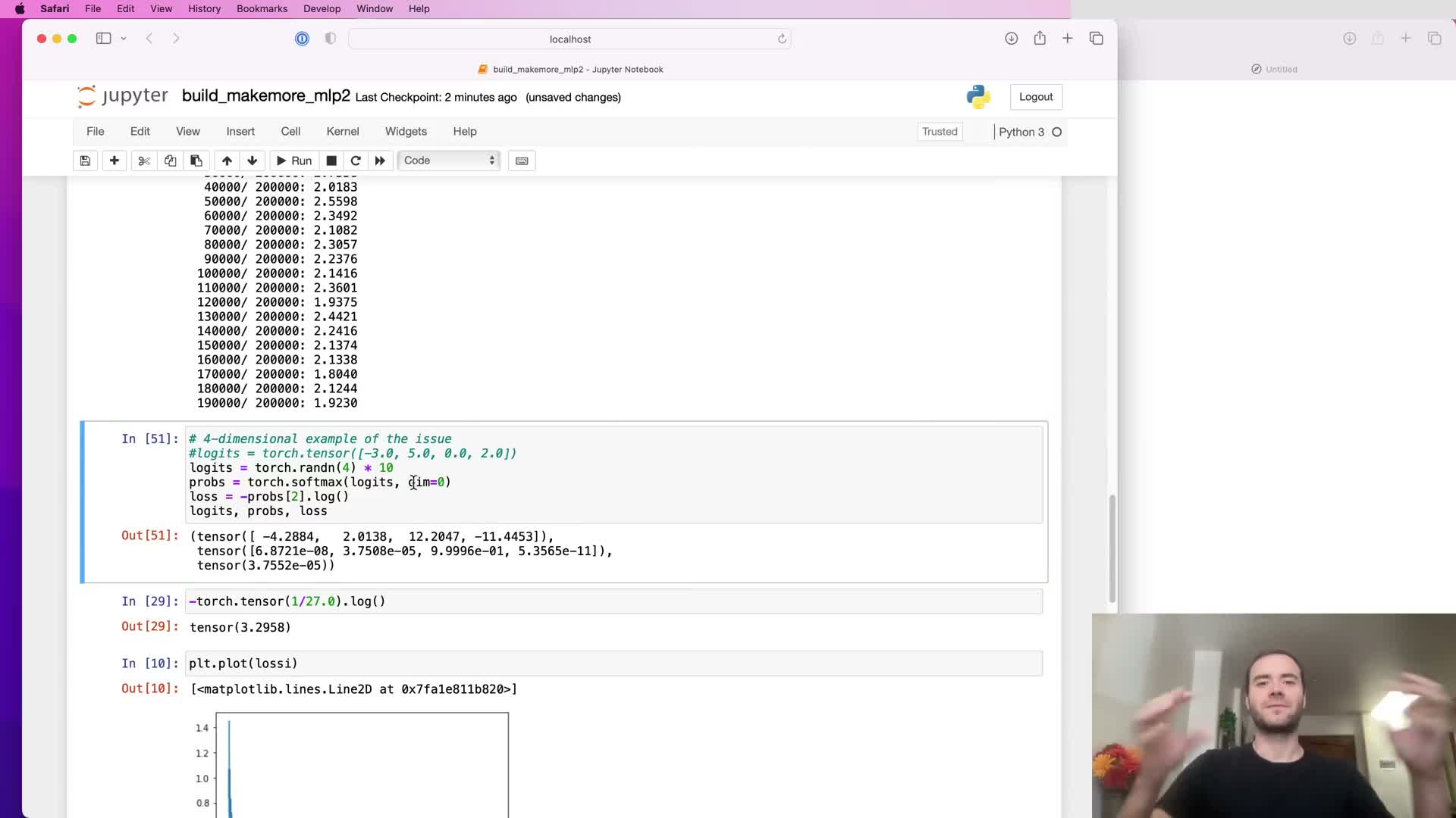
Random biases and large output weights can create extreme logits and overconfident wrong predictions at initialization.
Practical adjustments to avoid extreme initial logits:
- Set the output bias vector to zero.
- Scale down the output weight matrix by a modest factor (e.g., 0.01–0.1) so initial logits stay near zero.
- Keep small nonzero random weights (avoid exact zeroing) so symmetry breaking remains possible for gradient-based learning.
These pragmatic steps preserve slight randomness for optimization while preventing wasteful early corrective updates that arise from overconfident initial predictions.
Training dynamics after fixing output-layer scaling (hockey-stick effect)
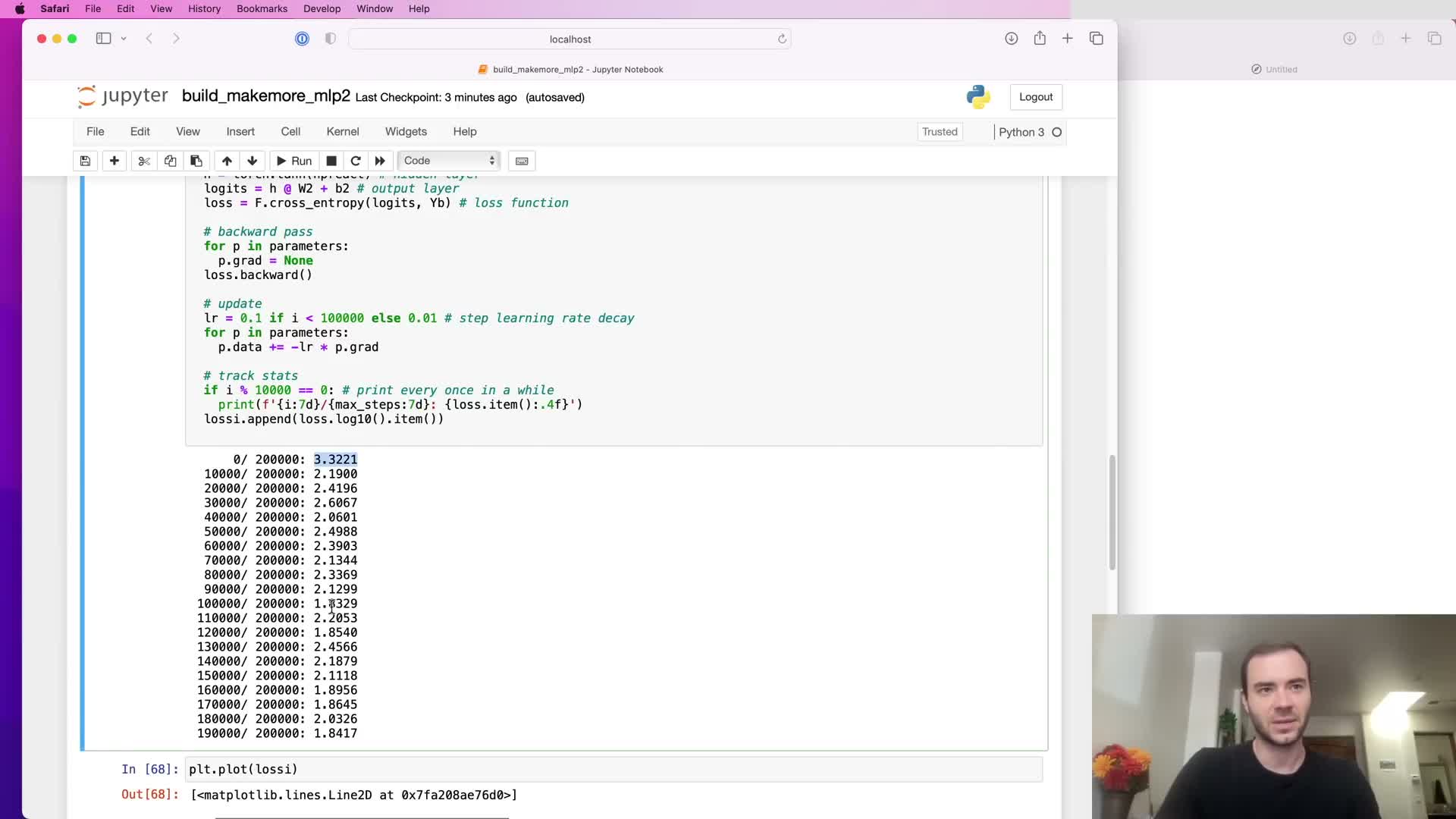
When output logits are initialized to extreme values, training often shows an initial fast phase where the optimizer simply collapses logits toward zero — the so-called “hockey-stick” descent.
With corrected output-layer scaling this trivial early phase disappears, so early loss descent more accurately reflects substantive model learning instead of just correcting overconfidence.
The result is more effective use of training iterations and typically improved final validation metrics because fewer steps are wasted on trivial fixes.
Tanh hidden-layer saturation and its impact on gradients
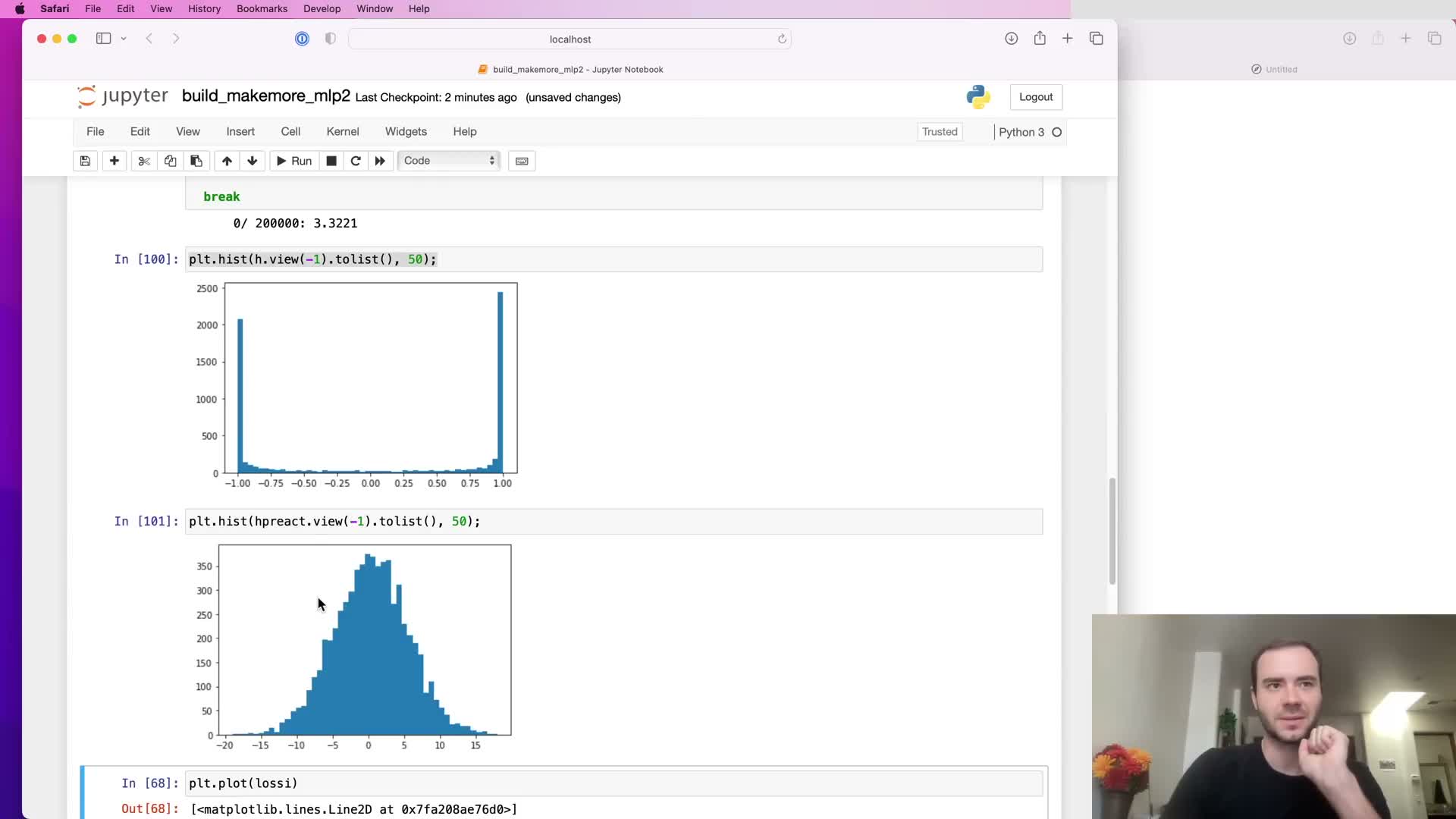
If pre-activation values feeding tanh are too large in magnitude then tanh outputs saturate near ±1, concentrating mass at the function tails.
Consequences of tanh saturation:
- Local derivative of tanh is 1 − t^2, which is near zero in the tails, so gradients are effectively killed during backpropagation.
- Learning stalls because those units stop contributing meaningful gradient signal.
- Visual diagnostics (histograms) reveal broad pre-activation ranges (e.g., ±15) and post-activation mass at ±1, indicating severe saturation.
This reduces effective gradient flow across the layer and is especially harmful in deeper networks where vanishing compounds across layers.
Dead neurons and nonlinearity-specific failure modes
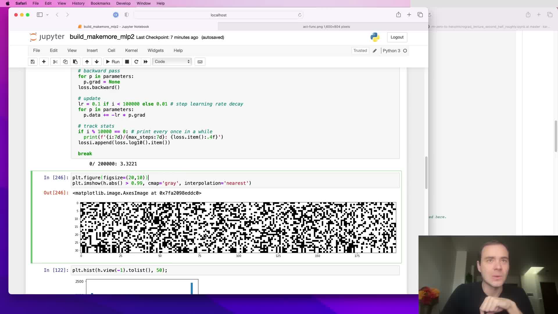
A neuron that produces saturated outputs for all inputs in the dataset (e.g., always tanh ≈ ±1 or ReLU ≤ 0) receives zero gradient and becomes permanently “dead” because its weights no longer affect the loss.
Where dead neurons come from and how they differ by nonlinearity:
-
tanh / sigmoid: saturated tails with near-zero derivatives.
-
ReLU: hard zero region for negative pre-activations (can produce permanently inactive units).
-
Leaky ReLU / ELU: mitigate but do not fully eliminate the risk of ineffective units.
Detecting dead neurons:
- Inspect per-neuron activation statistics across a batch or dataset.
- Columns (neurons) that are consistently saturated indicate dead units that will not recover under standard gradient-based updates.
Mitigating hidden-unit saturation by scaling weights and biases
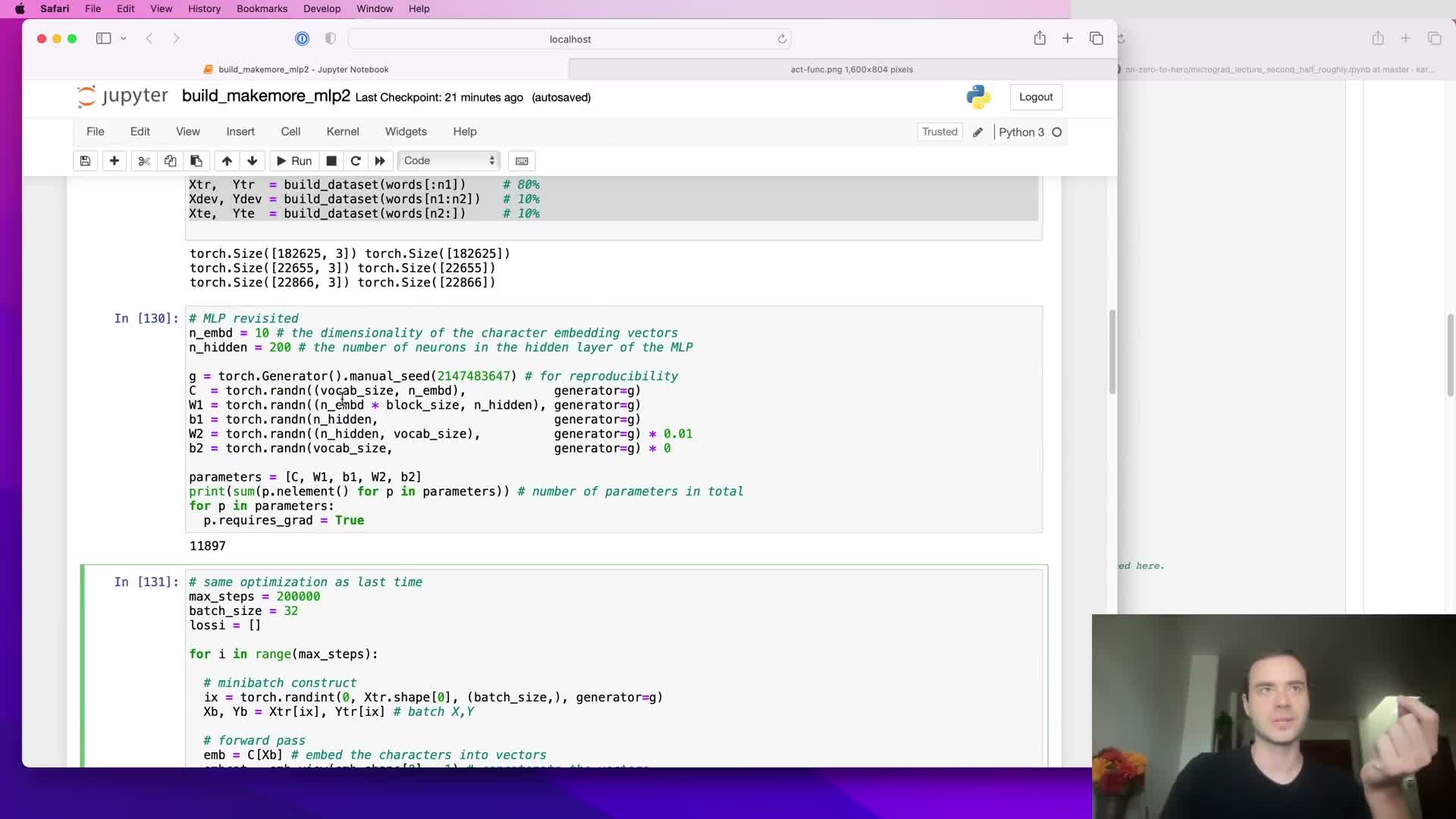
Pre-activation magnitudes arise from inputs multiplied by input-to-hidden weights plus biases; controlling those initialization scales prevents widespread saturation.
Practical initialization adjustments:
- Reduce the initialization scale of input-to-hidden weights (and optionally shrink biases).
- Multiply weight matrices and biases by a factor such as 0.1 to contract pre-activation variance from very large values to a controlled range (e.g., ±1.5).
- Retain small randomized biases to preserve symmetry breaking while avoiding saturation.
These steps produce more favorable activation histograms and preserve gradient flow, improving convergence in practice.
Empirical demonstration of initialization improvements on validation loss
Applying the pragmatic fixes — zeroing output biases, scaling output weights, and scaling input-to-hidden weights — reduces initial pathological loss behavior and produces a meaningful reduction in final validation loss (for example, from ~2.17 to ~2.10 in the demonstrated MLP).
Why this works:
- Fewer early iterations are spent correcting gross initialization artifacts.
- More iterations are allocated to fitting task-relevant structure.
- Absolute gains depend on model capacity and task, but the example shows how initialization choices materially affect optimization progress.
Principled variance preservation via fan-in scaling (Xavier/Kaiming motivation)
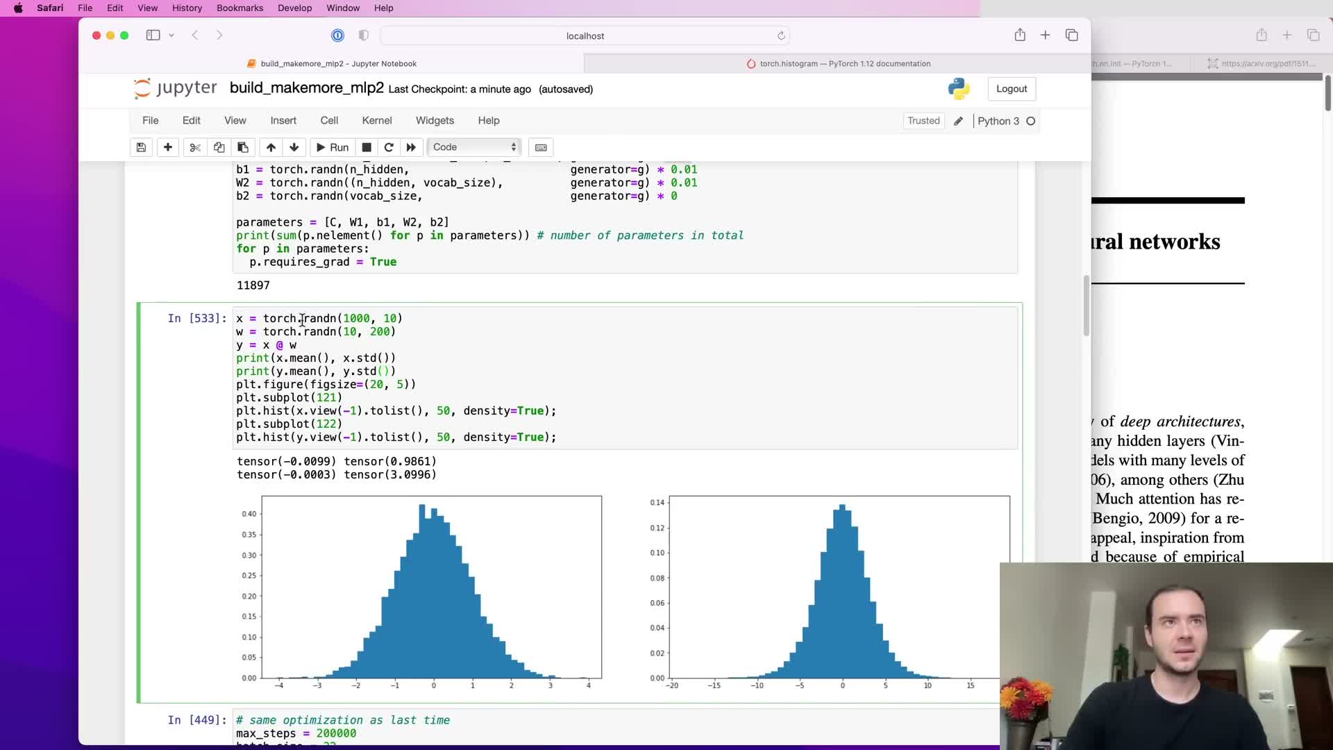
When inputs and weights are independent zero-mean random variables, the output variance after a linear transform scales with the number of input dimensions.
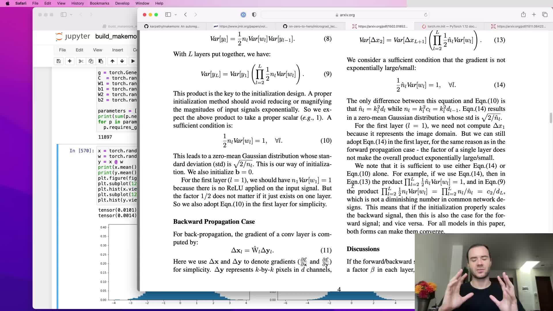
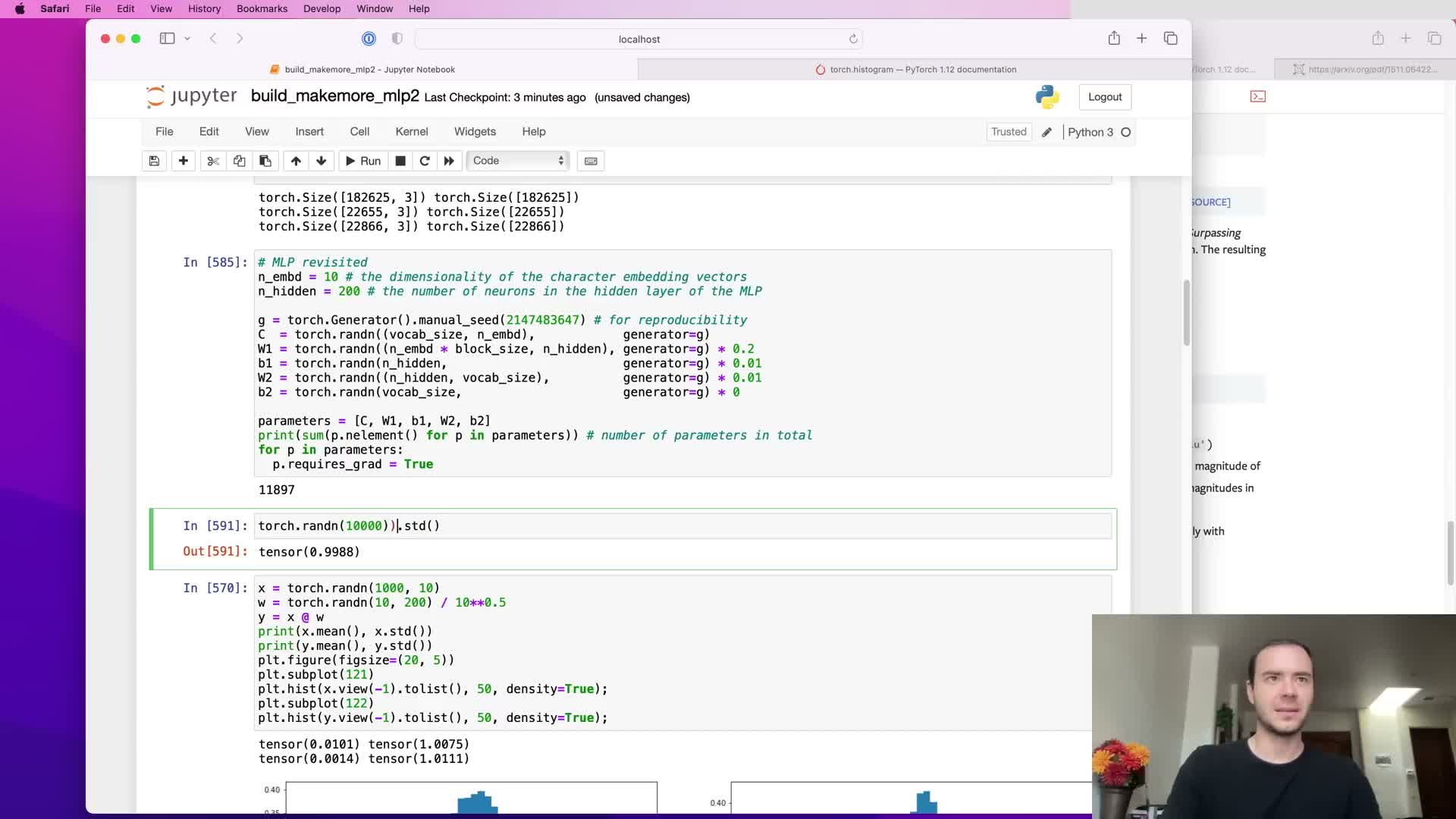
To preserve a stable activation variance one scales initial weights by 1/sqrt(fan_in).
This variance analysis ensures activations neither explode nor vanish layer-to-layer in deep linear stacks, making 1/sqrt(fan_in) a principled baseline for initializing dense or convolutional weight tensors and reducing the need for layer-specific tuning as depth increases.
Adjusting initialization gains for nonlinearities and He/Kaiming initialization
Nonlinear activation functions change forward and backward signal variances.
For ReLU-like nonlinearities that zero roughly half the distribution, the recommended Gaussian standard deviation is sqrt(2/fan_in) (the He/Kaiming initialization) to compensate.
Notes on gains and PyTorch:
- Different nonlinearities require different multiplicative gains to balance contraction/expansion.
- PyTorch initializers accept a gain parameter tied to the nonlinearity (e.g., gain=√2 for ReLU).
- Correct gain selection helps keep both activations and gradients well-scaled through deep networks.
Modern mitigations that relax fragile initialization requirements
Later innovations make precise initialization less fragile:
-
Residual connections add identity pathways that alleviate signal attenuation.
-
Normalization layers (batch, layer, group, instance) actively control activation statistics during training.
- Superior optimizers (RMSprop, Adam) adapt gradient steps per-parameter.
These techniques reduce sensitivity to exact initial variance scaling and enable deeper architectures to train reliably with simpler initialization heuristics, though principled initialization remains a useful baseline for stability and speed.
Batch normalization: standardizing activations per batch to control statistics
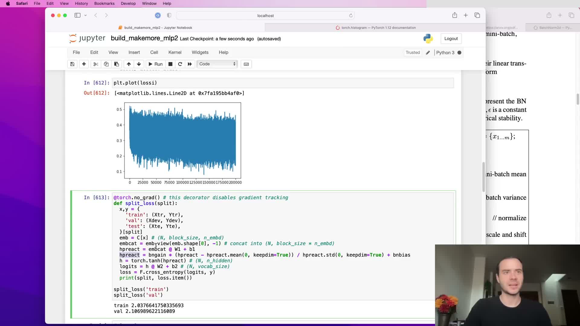
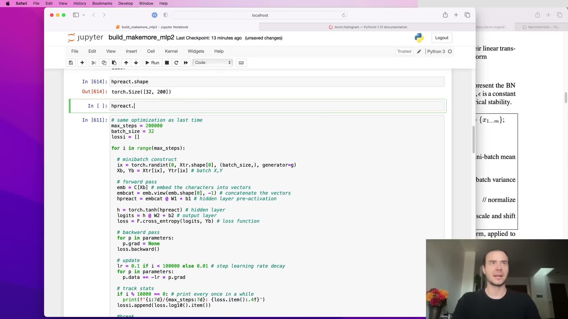
Batch normalization standardizes layer pre-activations by subtracting the batch mean and dividing by the batch standard deviation, producing per-feature activations with zero mean and unit variance across the mini-batch.
Key properties:
- The operation is differentiable and inserted into the computational graph so gradients flow through the normalization.
- It enforces well-scaled activations during training and mitigates saturation and internal covariate shift across layers.
- Because normalization is applied per mini-batch, it constrains activations to a predictable distribution and stabilizes deep network training dynamics.
Learned scale and shift (gamma and beta) and avoiding permanent Gaussian forcing
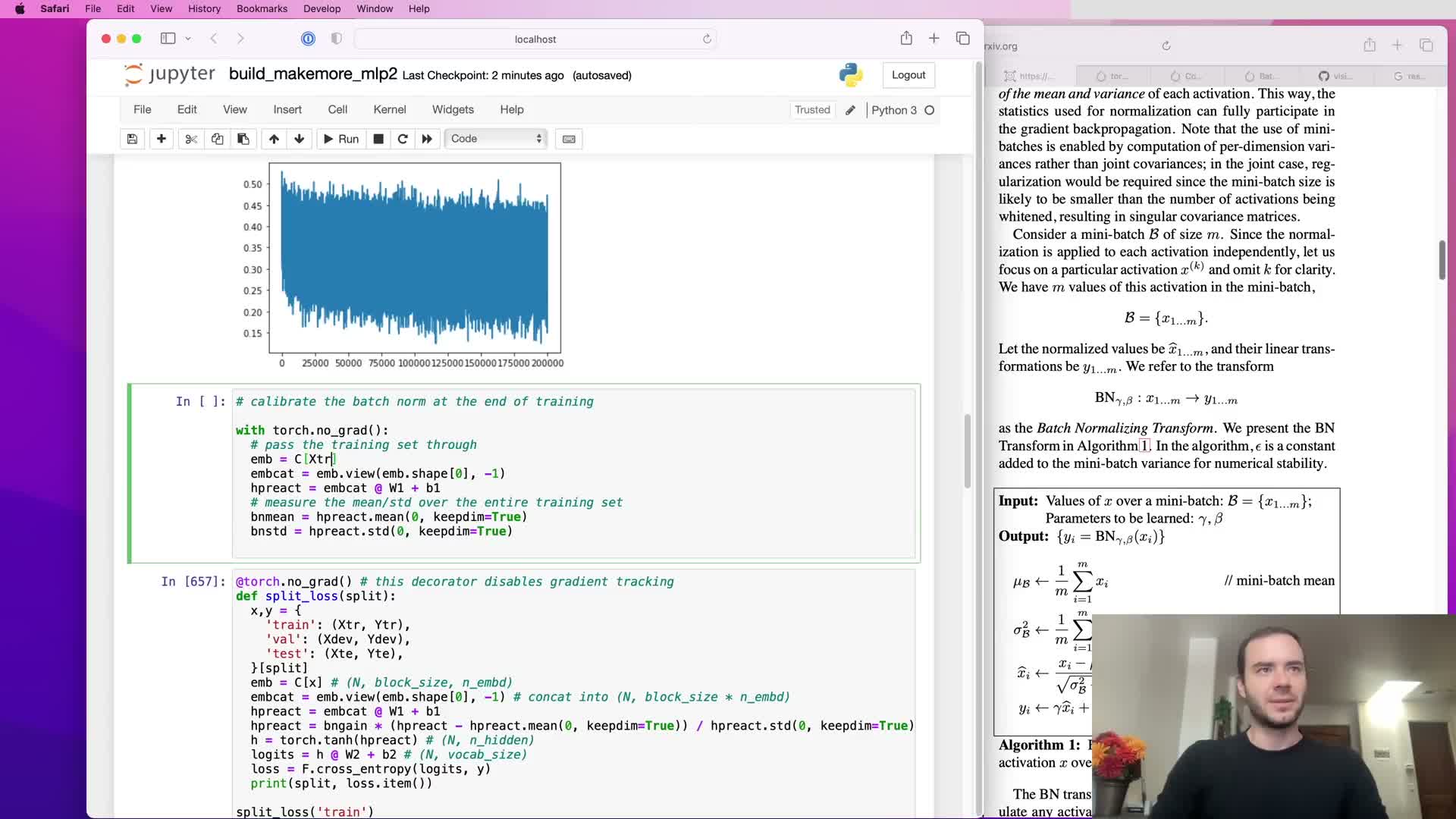
To permit the network to recover arbitrary useful distributions, BatchNorm follows standardization with a learned per-feature scale (gamma) and shift (beta).
Typical defaults and rationale:
- Initialize gamma to ones and beta to zeros so the initial behavior is unit Gaussian.
- Training can reshape each feature’s distribution via backpropagation, preserving expressivity while retaining the stabilization benefits of normalization.
BatchNorm inference: calibration, running statistics, and no-grad updates
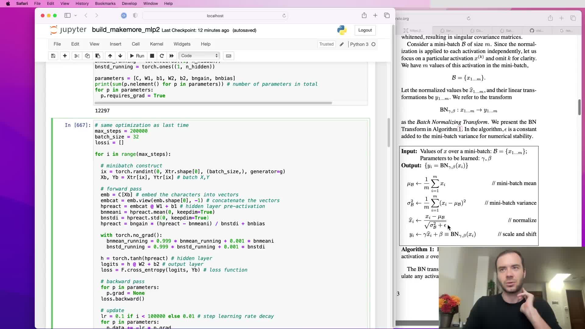
Because batch normalization depends on batch statistics, inference on single examples requires fixed estimates of per-feature mean and variance.
How those estimates are obtained and used:
- Calibrate by a post-training pass over the training set or accumulate online via exponential moving averages (running mean and running variance) during training.
- Update running estimates with a small momentum outside the gradient graph (use a no_grad context) so they do not participate in backpropagation.
- Use the running estimates at evaluation time to normalize single examples deterministically.
This design enables one-stage training without a separate calibration pass while preserving correct inference behavior.
Numerical safeguards, parameter/buffer semantics and bias handling with BatchNorm
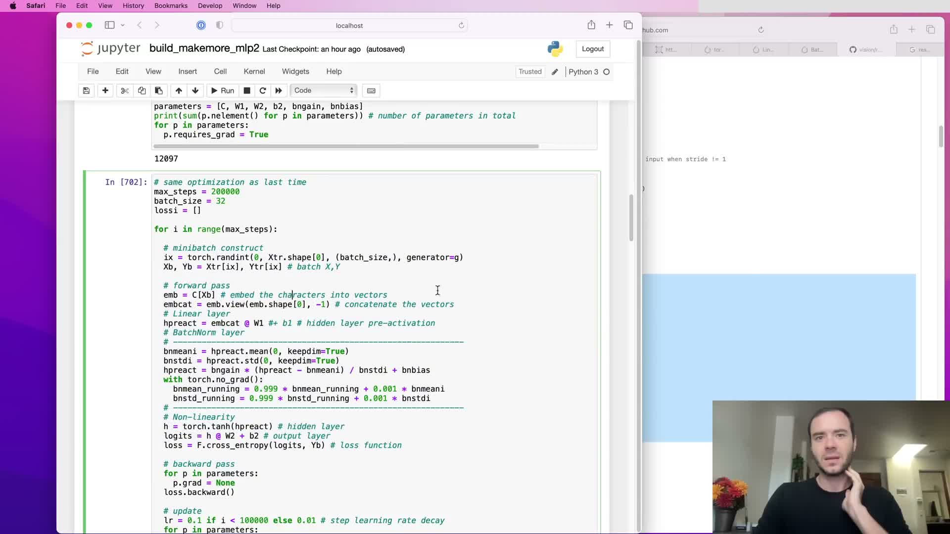
BatchNorm implementations include a small epsilon in the denominator to avoid division-by-zero when variance is extremely small, ensuring numerical stability.
Practical notes:
- Layers immediately preceding a BatchNorm typically disable their own bias terms because those biases are cancelled by the BatchNorm mean subtraction and therefore become redundant and receive zero gradients.
- PyTorch distinguishes trainable parameters (gamma/beta) from buffers (running mean/variance) to reflect that running statistics are updated outside gradient-based optimization and should not be included in parameter gradient updates.
ResNet design pattern and typical placement of BatchNorm
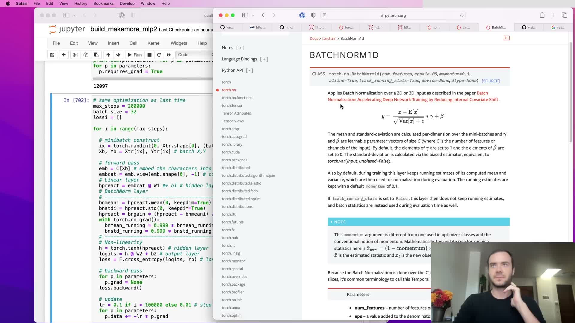
Modern convolutional architectures (e.g., ResNet) adopt a recurring motif: convolution → BatchNorm → nonlinearity (often ReLU) repeatedly, sometimes with residual identity shortcuts between blocks.
Practical conventions in these blocks:
- Convolutional layers commonly set bias=False because BatchNorm provides the necessary affine shift.
- BatchNorm is usually applied right after the convolution and before the activation.
This pattern standardizes internal feature statistics across depth and enables very deep models to be trained robustly — it underlies many state-of-the-art vision architectures.
PyTorch layer conventions and default initialization behavior
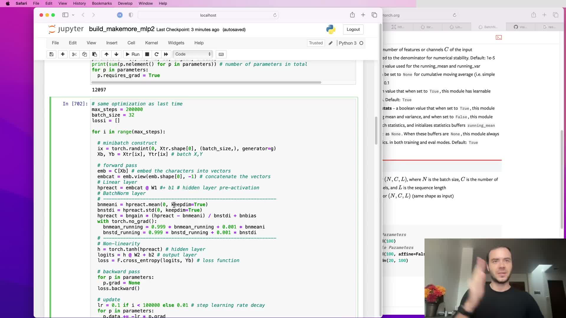
PyTorch linear and convolutional modules expose fan_in/fan_out-derived initialization defaults that sample weights from uniform distributions scaled by 1/sqrt(fan_in) (or variants) and initialize biases to zero if enabled.
BatchNorm modules expose useful arguments and defaults:
-
epsilon (for numerical stability).
-
momentum (for running statistics updates).
-
affine flag (whether to learn gamma/beta).
-
track_running_stats (whether to maintain running mean/variance).
Understanding these defaults allows developers to rely on well-tested initialization strategies and tune momentum or epsilon only when necessary (e.g., small batches or special numerical circumstances).
Need for diagnostics and overview of pyTorch-like modularization
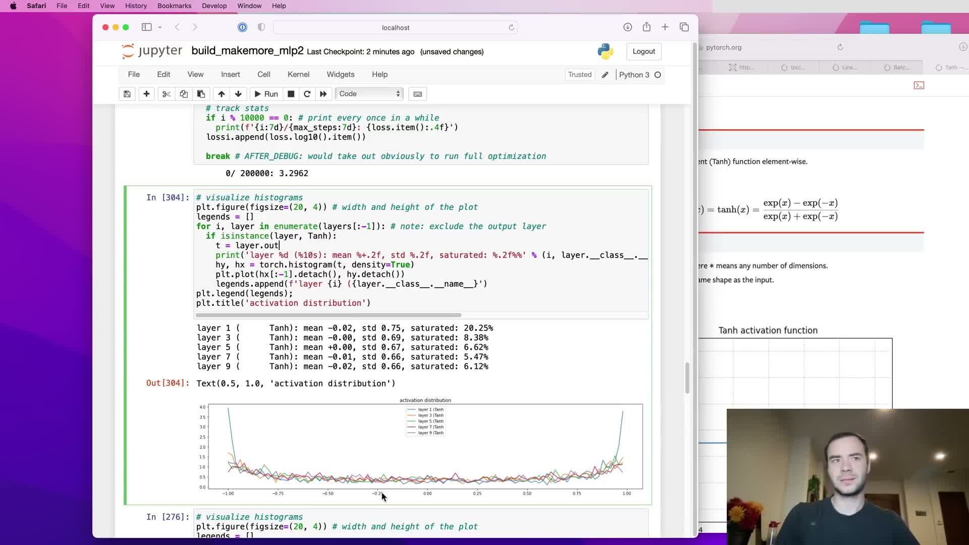
Refactoring model code into modular layer classes (e.g., Linear, BatchNorm1d, Tanh) mirrors PyTorch’s API and simplifies instrumentation and diagnostics by providing consistent access to layer outputs and parameters.
Instrumentation and diagnostics benefits:
- Easy recording of forward activations (per-layer means, standard deviations, saturation rates).
- Access to backward gradients (distributions and magnitudes).
- Visibility into where gradients vanish or explode and detection of dead neurons.
These diagnostics form the basis for actionable fixes such as re-scaling initializations, adjusting learning rates, or inserting normalization layers.
Practical diagnostics: activation histograms, saturation metrics, gradient histograms, and parameter statistics
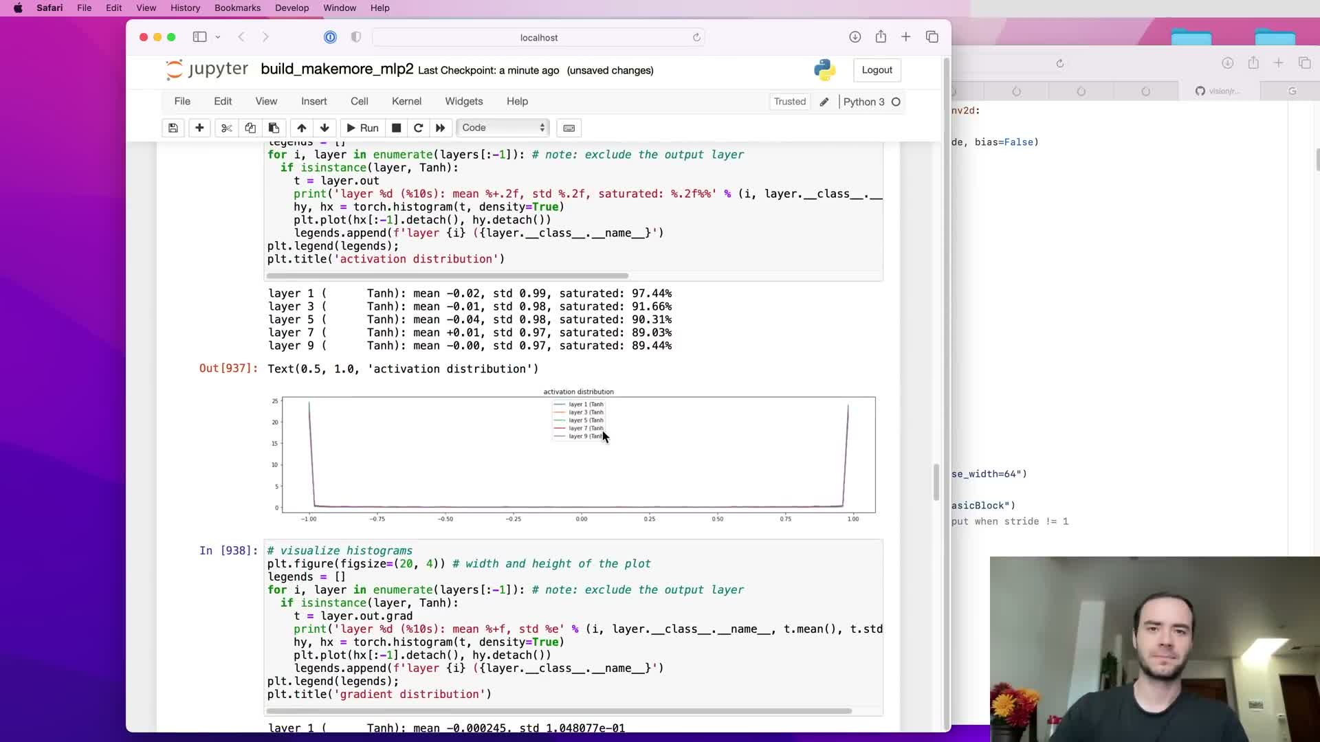
A practical diagnostic suite includes:
- Per-layer histograms of activations and gradients.
-
Per-layer saturation percentages (e.g., proportion of tanh outputs with t > 0.97).
- Parameter-level statistics such as weight histograms, parameter standard deviations, and gradient-to-parameter ratios.
Monitoring these metrics over iterations reveals trends like shrinking or exploding activations/gradients, layer-wise asymmetries, and disproportionate learning in specific layers.
These signals inform concrete interventions (change initial scaling, add BatchNorm, modify learning rate, or change optimizer) to restore homogeneity of forward and backward flows across the network.
Enjoy Reading This Article?
Here are some more articles you might like to read next: