Karpathy Series - Bulding Makemore Part 4 - Becoming a Backprop Ninja
- Manual tensor-level backward implementation exposes autograd internals and prevents silent failures
- Manual gradient programming was historically standard and facilitated numerical gradient checking in research code
- The notebook implements a two-layer MLP with batch normalization and a sequence of exercises to derive manual backward passes
- Gradient of the batch-averaged negative log-probabilities with respect to extracted log-probabilities equals -1/N at selected target indices and zero elsewhere
- The elementwise logarithm backpropagates by multiplying the upstream gradient by 1/probability, amplifying low-probability examples
- Softmax normalization backpropagates through exponentiation, a summation with broadcasting, and a numerically-stable max subtraction that has negligible gradient
- Backward pass through a linear (dense) layer is expressible as matrix multiplications and vector sums derived by shape matching
- The tanh activation backward uses the identity d/dx tanh(x) = 1 - tanh(x)^2, and batch-norm scale/shift parameters accumulate gradients across the batch
- Batch normalization forward computes per-feature mean and variance and the choice of normalization denominator (N vs N-1) changes bias properties
- Backpropagation through batch normalization requires careful topological ordering and handling of broadcasts, sums, and fan-outs
- Concatenation, reshape (view), and embedding lookup backward passes undo the forward indexing and accumulate repeated contributions
- The analytic gradient of cross-entropy with softmax simplifies to softmax probabilities minus a one-hot label and is scaled by the batch size mean
- Logits gradients act as per-row conservation ‘forces’ that push down incorrect probabilities and pull up the correct one with zero net sum
- The closed-form backward formula for batch normalization condenses many atomic derivatives into an efficient per-feature expression that uses batch-level statistics
- A complete manual backward pass assembled from validated component derivatives can replace autograd for training and yield equivalent results
Manual tensor-level backward implementation exposes autograd internals and prevents silent failures

Implementing backpropagation at the tensor level makes explicit the gradient computations that autograd otherwise hides, enabling precise debugging and avoidance of subtle bugs.
Writing manual backward passes clarifies how each intermediate tensor contributes to the loss and where gradients can vanish or explode—this is essential when diagnosing saturated activations, dead neurons, or incorrect gradient manipulations (for example, clipping the loss instead of clipping gradients).
Implementing tensor-level derivatives forces correct handling of broadcasting, accumulation, and numerical stability, and it serves as a pedagogical exercise that strengthens intuition about gradient flow.
This approach is not an argument against autograd in production; rather, it provides a concrete safety net and a deeper understanding for debugging and for designing architectures.
Manual gradient programming was historically standard and facilitated numerical gradient checking in research code

Historically, researchers wrote explicit backward passes because auto-differentiation frameworks were not broadly available.
Common workflows used languages like Matlab or early numpy code to compute gradients and updates manually. Techniques such as contrastive divergence and bespoke gradient estimators required inline manipulation of gradients and parameter updates.
As a result, a gradient-checking tandem of analytic and numerical gradients became standard practice.
Implementing manual backward computations encourages construction of numerical gradient checks (finite-difference checks) to validate analytic derivatives before large-scale experiments.
This historical perspective shows manual differentiation’s role in rigorous model development and in building intuition about when and why gradients behave pathologically.
The notebook implements a two-layer MLP with batch normalization and a sequence of exercises to derive manual backward passes
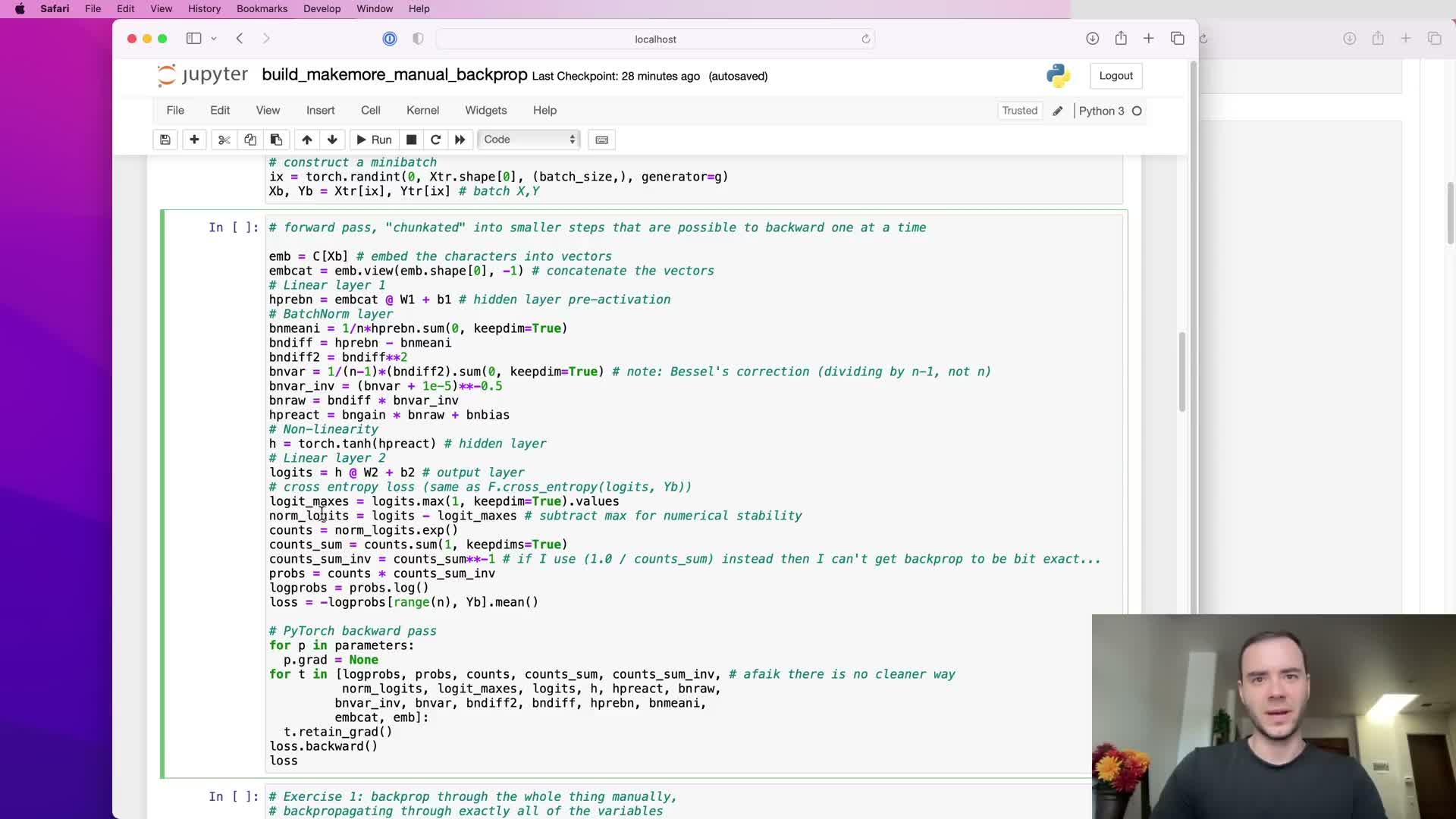
The working environment defines a two-layer multilayer perceptron (MLP) with the following components:
-
Embedding table
-
First linear layer
-
Batch normalization
-
tanh nonlinearity
-
Second linear layer
- An explicit cross-entropy loss
The notebook provides starter code, utilities to compare manual versus PyTorch gradients, and small-bias random initialization to unmask implementation errors.
Intermediate tensors are retained during the forward pass so their derivatives can be computed and compared.
A helper function compares elementwise equality and the maximum difference between manual and autograd gradients.
The course of work is organized into exercises:
- Backprop through the fully decomposed loss graph.
- Derive the analytic cross-entropy gradient with respect to logits.
- Derive an efficient batch-normalization backward formula.
- Assemble the full manual training loop and compare results with autograd.
Gradient of the batch-averaged negative log-probabilities with respect to extracted log-probabilities equals -1/N at selected target indices and zero elsewhere
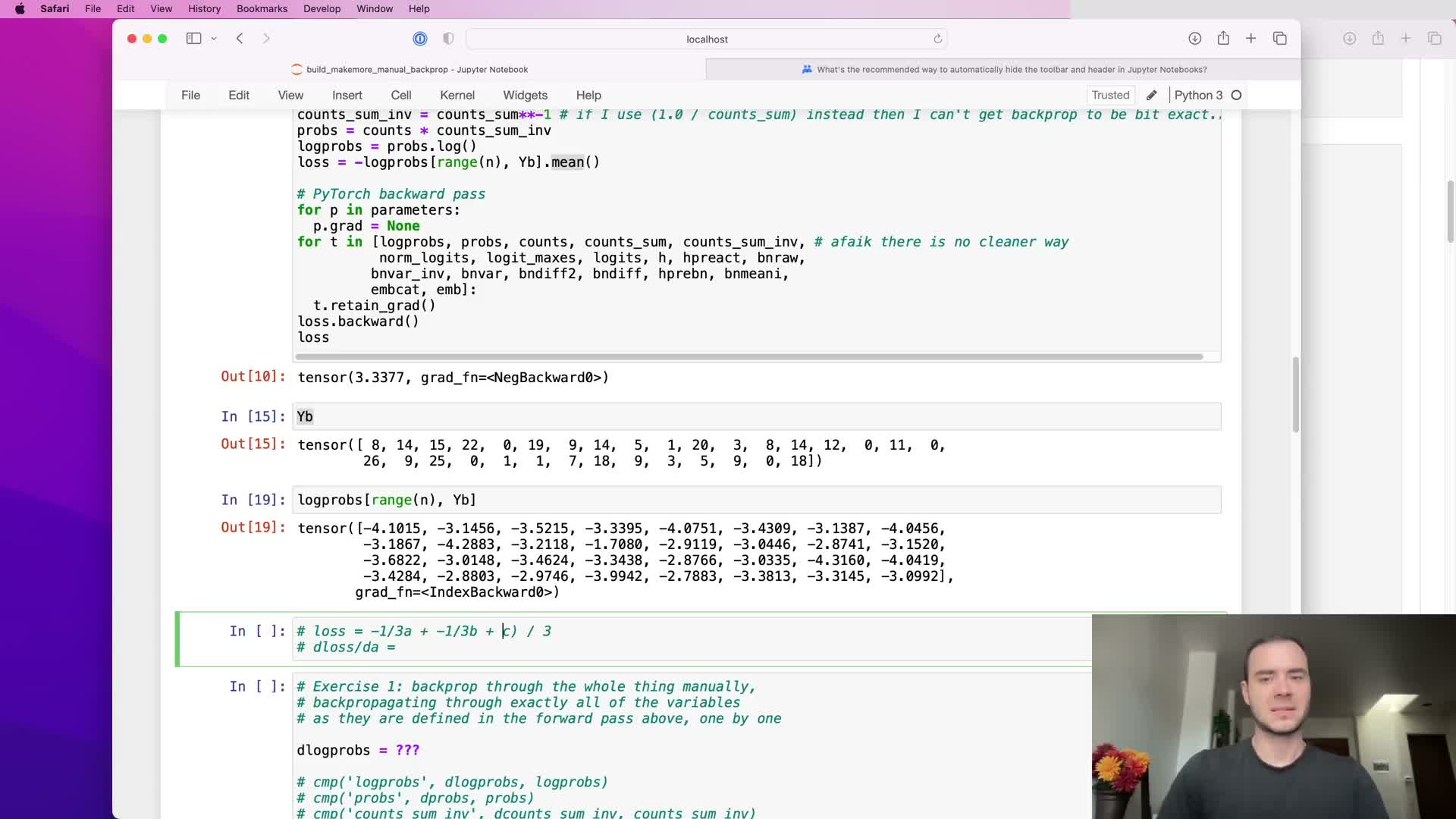
When the loss is computed as the mean negative log-probability of the correct class across a batch, the derivative with respect to each extracted log-probability (one per example) is:
-
-1/N at the positions selected by the label indices
-
0 for all other logit locations
Shape consistency requires the gradient tensor to match the log-probabilities tensor (e.g., batch_size × num_classes).
Implementation pattern:
- Initialize with zeros_like(log_probs).
- Assign -1.0 / N to the indexed positions corresponding to the ground-truth labels.
This derivative is straightforward, cheap to implement, and serves as the base of the chain rule for backpropagating through subsequent layers.
Validate it against autograd using exact or allclose comparisons.
The elementwise logarithm backpropagates by multiplying the upstream gradient by 1/probability, amplifying low-probability examples
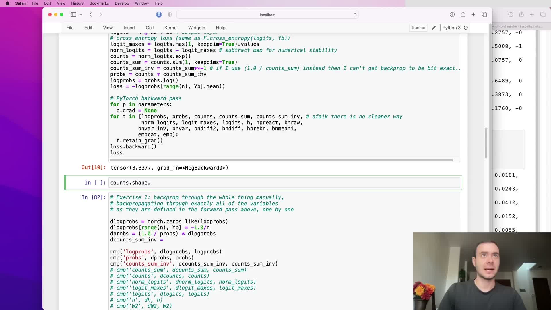
For an elementwise log operation y = log(x) the local derivative is dy/dx = 1/x, so the gradient flowing into the predecessor tensor is the upstream gradient multiplied elementwise by 1/x.
In the cross-entropy–softmax decomposition this means gradients associated with very small predicted probabilities are amplified (1 / small_value), which increases the corrective signal for severely underpredicted true classes.
Implementation note:
- Compute this as an elementwise multiply of d_log_probs by 1.0 / probs (or probs.reciprocal()).
- Respect the original tensor shapes and broadcasting semantics.
This step highlights why numerical stability and correct probability handling matter in the backward pass.
Softmax normalization backpropagates through exponentiation, a summation with broadcasting, and a numerically-stable max subtraction that has negligible gradient
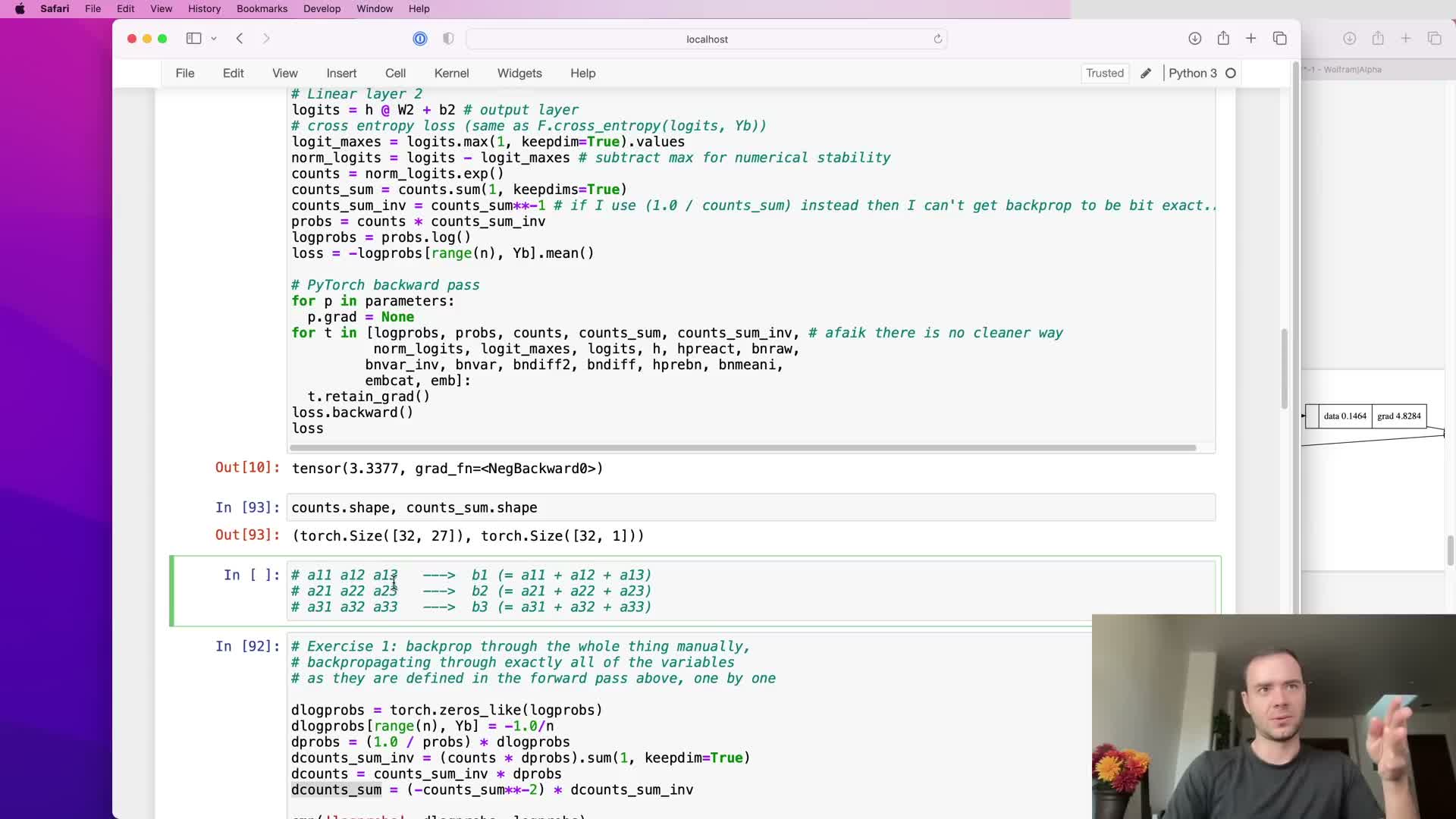
Softmax is implemented as:
-
counts = exp(logits - max_per_row) (subtract per-row max for numerical stability)
-
probs = counts * (count_sum_inverse) where count_sum_inverse = 1 / sum(counts)
Backpropagation follows from elementwise derivatives:
- d(exp(x))/dx = exp(x)
- d(1/sum)/dsum = -1 * sum^{-2} (power rule)
Practical considerations:
- When tensors are broadcast (e.g., a column vector of sums broadcast across columns), the backward pass must account for tensor replication by summing gradients across the broadcasted dimension.
- When a scalar or row is reused across columns, gradients from each use are summed into the original variable.
- The subtraction of the per-row maximum for numerical stability does not change the softmax output; it yields gradients that are theoretically zero and only produce tiny floating-point residuals in practice.
- Careful shape reasoning (for example, use of keepdim in sums and appropriate transposes) is required to preserve correspondence with autograd.
Backward pass through a linear (dense) layer is expressible as matrix multiplications and vector sums derived by shape matching
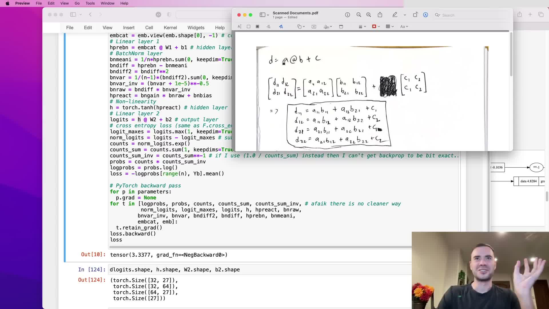
For a linear forward pass D = H W + b with shapes:
- H: (batch, Nhidden)
- W: (Nhidden, Nclasses)
- b: (Nclasses,)
the backward propagation reduces to:
-
dH = dD W^T
-
dW = H^T dD
-
db = sum_rows(dD) (sum over the batch axis)
These formulas follow from expanding scalar dot-products in the forward pass and applying the chain rule elementwise, then recognizing the summed contributions as matrix multiplications plus appropriate transpositions.
Shape analysis yields which transpose and summation axes must be used—only one configuration makes the matrix dimensions conform.
Implement these formulas using efficient BLAS-backed matrix operations and verify by comparing to autograd gradients.
The tanh activation backward uses the identity d/dx tanh(x) = 1 - tanh(x)^2, and batch-norm scale/shift parameters accumulate gradients across the batch
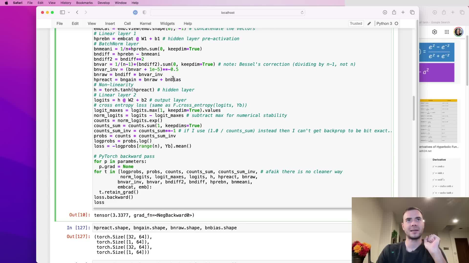
For a tanh nonlinearity a = tanh(z) the local derivative is da/dz = 1 - a^2, where a is the tanh output.
- The upstream gradient is multiplied elementwise by (1 - a^2) to yield dZ.
- Computing this using the activation output avoids recomputing hyperbolic functions of the input.
In batch normalization, the affine parameters are handled simply:
-
dgamma = sum_over_batch(d_pre-activation * x_hat)
-
dbeta = sum_over_batch(d_pre-activation)
These sums must respect the broadcasting that occurred in the forward pass and typically collapse the batch dimension while retaining feature dimensionality.
Implementation must ensure correct use of keepdim or reshape so that gamma/beta gradients have the intended shapes and can be applied in parameter updates.
Batch normalization forward computes per-feature mean and variance and the choice of normalization denominator (N vs N-1) changes bias properties
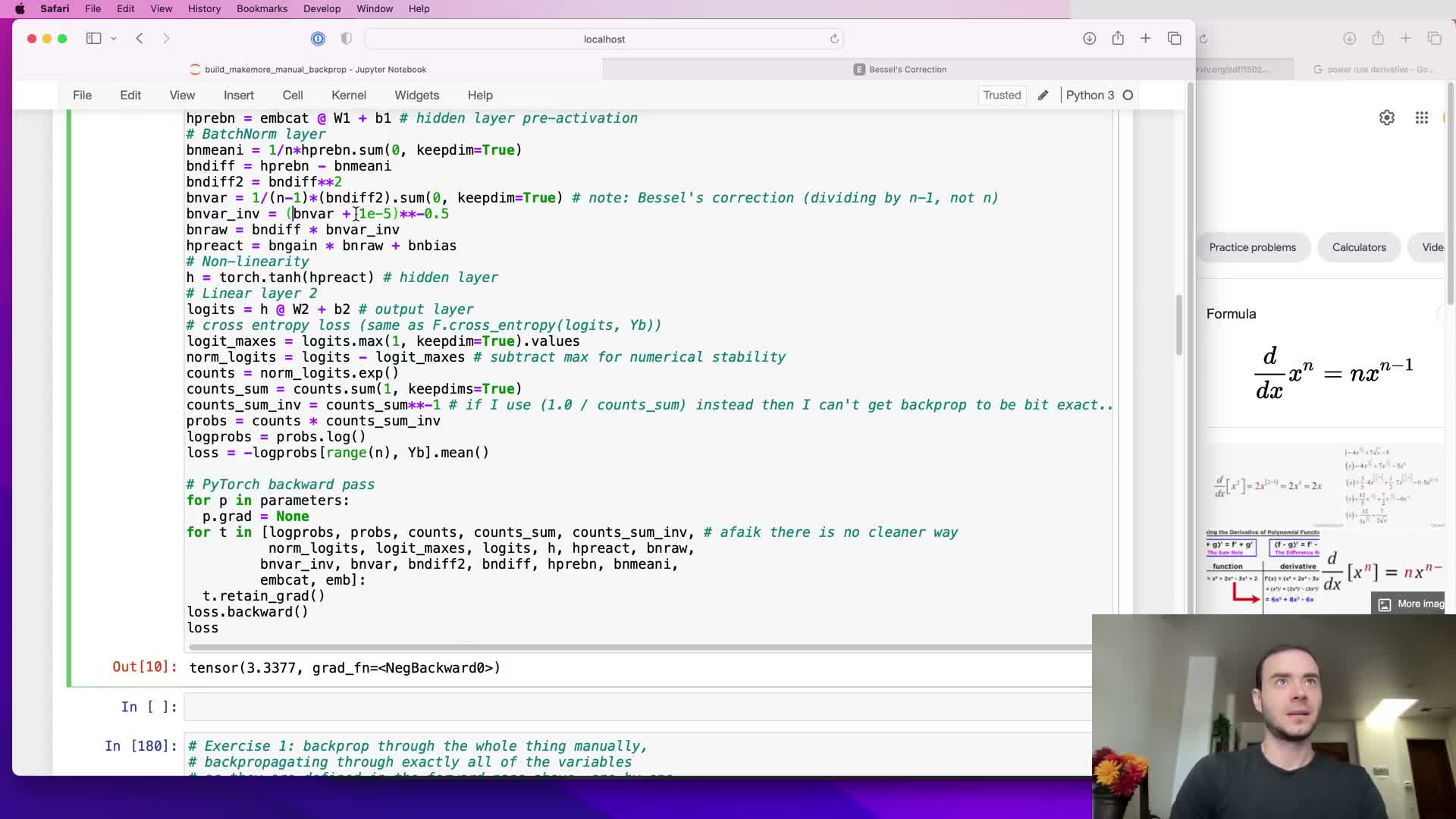
Batch normalization decomposes into the following steps:
- Per-feature mean: mu = (1/m) sum x
- Centered differences: x - mu
- Variance estimate: sigma^2 = (1/(m-1)) sum (x - mu)^2 (or biased 1/m alternative)
- Regularization with epsilon to prevent divide-by-zero
- Inverse square-root scaling to produce x_hat = (x - mu) * (sigma^2 + eps)^{-1/2}
Implementation decision point:
- Using (N-1) (Bessel correction) produces an unbiased variance estimator for small sample sizes and avoids systematic underestimation that the biased 1/N estimator produces.
- This choice affects training-time statistics and the calibration of running means/variances used at inference.
- Some frameworks historically mix biased estimation at training and unbiased at inference, creating a train–test mismatch; consistent use of an unbiased estimator (1/(N-1)) is recommended for small mini-batches.
Numerically, epsilon prevents divide-by-zero and the inverse-root is efficiently implemented as a power -0.5, followed by broadcasting to align feature dimensions.
Backpropagation through batch normalization requires careful topological ordering and handling of broadcasts, sums, and fan-outs

The backward pass for batch normalization is implemented by traversing the computational graph in topologically sorted order:
- Propagate gradients from dY to dX_hat (via gamma).
- Propagate from dX_hat to d_var and d_mu.
- Finally compute dX, because mu and var are shared scalars that fan out into many X_hat nodes.
Key implementation points:
- Operations that summed across the batch during the forward pass imply replication in the backward pass and vice versa.
- Gradients that come from replicated uses must be summed along the same axis used for reduction (often the batch axis with keepdim semantics).
- A practical implementation constructs intermediate gradients with zeros_like, uses ones-matrix multiplications to replicate or broadcast, and accumulates contributions from multiple branches using += to account for fan-outs.
Check each intermediate against autograd to ensure correctness.
Concatenation, reshape (view), and embedding lookup backward passes undo the forward indexing and accumulate repeated contributions
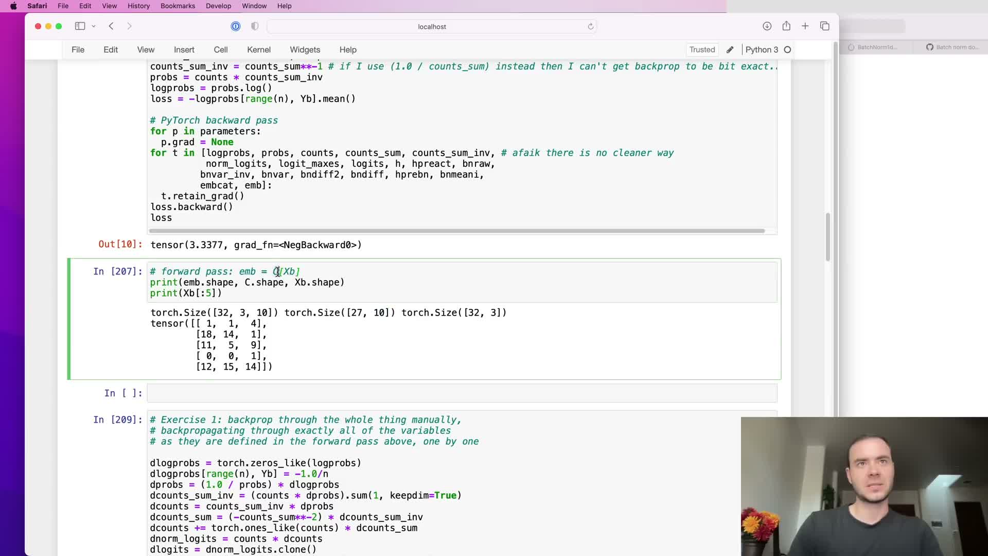
Reshaping (view) is a no-op with respect to memory layout, so the backward pass simply reshapes the upstream gradient back to the original operand shape (e.g., call .view(original_shape) on the gradient).
For concatenation or explicit stacking that created a larger tensor from smaller tensors, the backward pass slices the upstream gradient to match each original component and assigns those slices to the corresponding gradient variables.
An embedding lookup performed via integer indexing maps rows of an embedding matrix into a batched tensor; the backward pass reverses this by:
- Initializing an embedding gradient matrix of zeros.
- For each lookup index, adding the corresponding vector gradient into the embedding gradient row (accumulating with += if an index appears multiple times).
When a vectorized scatter-add operation is available it is preferred; otherwise a loop that accumulates contributions is correct and must preserve shapes.
The analytic gradient of cross-entropy with softmax simplifies to softmax probabilities minus a one-hot label and is scaled by the batch size mean
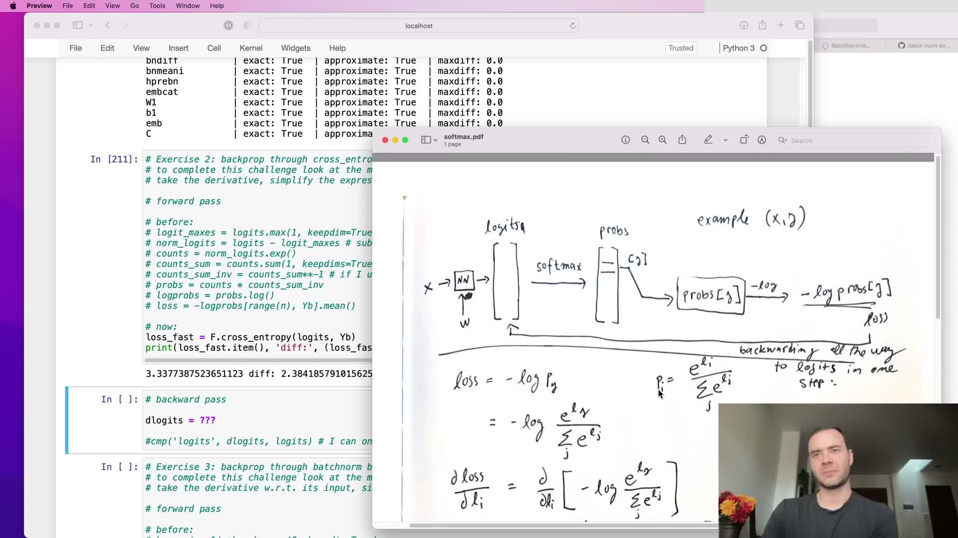
For a single example with softmax probabilities p = softmax(logits) and true label y, the derivative of the negative log-likelihood with respect to logits is:
- ∂L/∂logit_i = p_i for i ≠ y
- ∂L/∂logit_y = p_y − 1
This compact form arises after differentiating the softmax and log and canceling common terms.
For a batch loss computed by averaging over N examples, this gradient is additionally divided by N.
Implementation recipe:
- Compute p across rows.
- Subtract 1 at the ground-truth indices.
- Divide by the batch size.
This analytic expression is far more efficient than decomposing the loss into many atomic ops and backpropagating through each step, and it matches autograd to floating-point tolerance.
Logits gradients act as per-row conservation ‘forces’ that push down incorrect probabilities and pull up the correct one with zero net sum
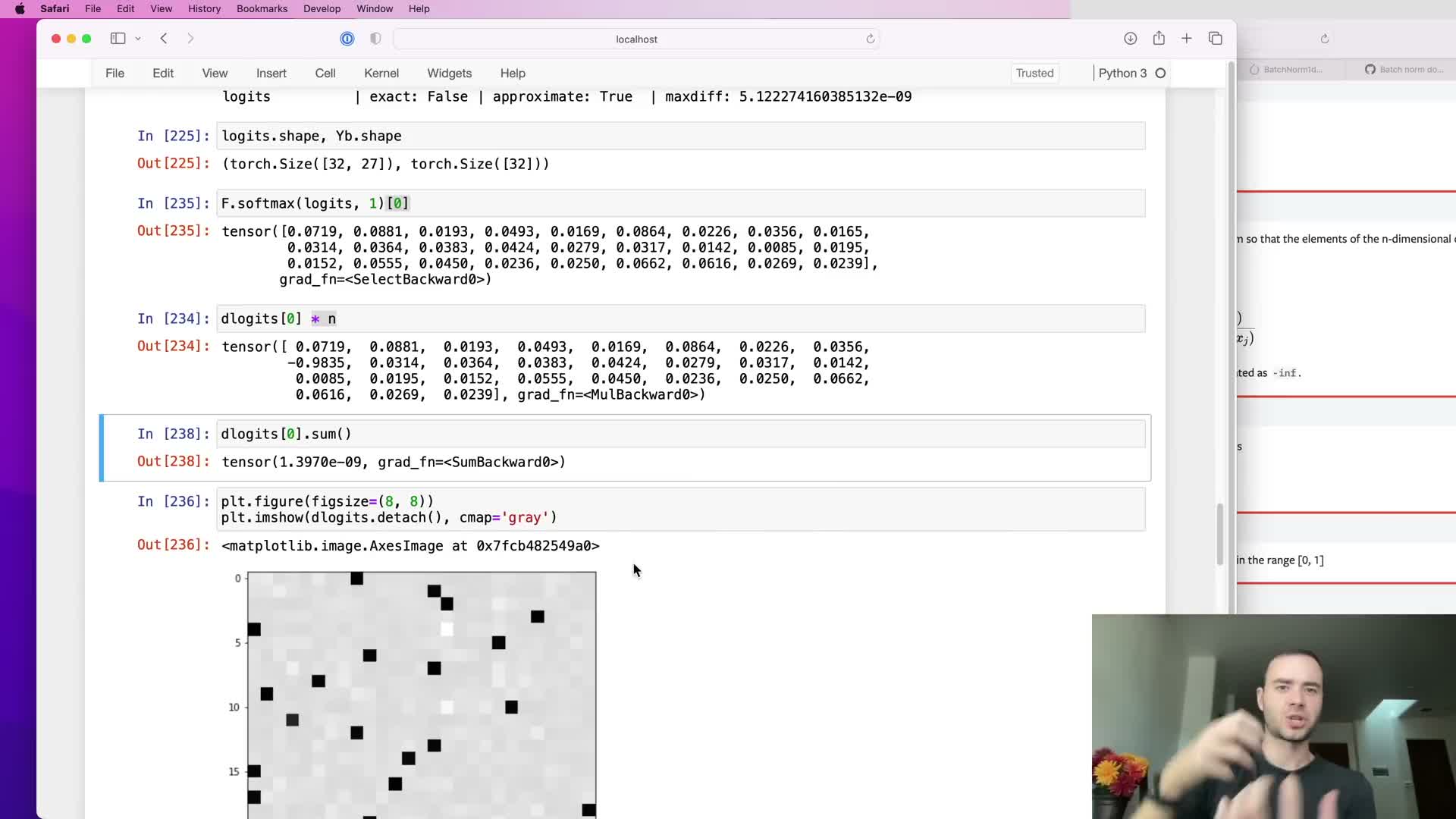
The gradient vector for each example’s logits can be interpreted as a set of forces that conserve mass:
- The per-class gradient entries sum to zero, meaning the total probability mass is redistributed rather than created or destroyed.
- Each incorrect class receives a negative pull proportional to its predicted probability p_i.
- The true class receives a positive push of magnitude 1 − p_y.
Thus, confident mispredictions produce large corrective gradients. This physical metaphor explains why gradient magnitudes reflect both the confidence and the correctness of predictions and clarifies how local manipulations at the logits propagate through the network to update parameters.
The closed-form backward formula for batch normalization condenses many atomic derivatives into an efficient per-feature expression that uses batch-level statistics
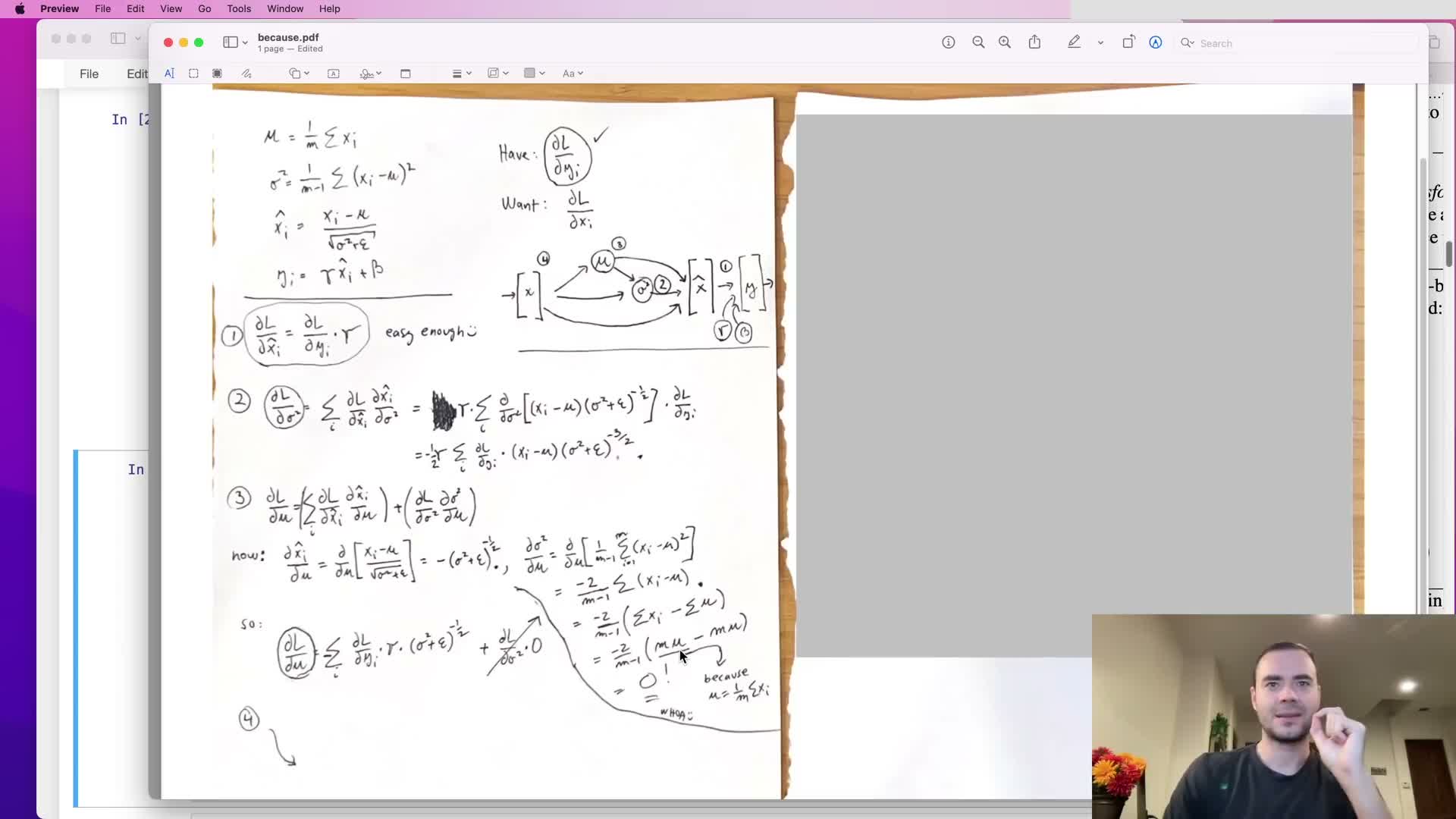
Deriving dL/dX for batch-normalized activations yields a compact vectorized expression that combines:
- The upstream gradient
- The per-feature inverse-standard-deviation factors
- The mean of upstream gradients over the batch
- Inner products with the centered inputs
Algebraic simplification consolidates terms involving (var + eps)^{-3/2} and sums over batch elements into three additive components.
The final formula computes the gradient in parallel for all features by using elementwise multiplications, reductions (sums) over the batch axis, and appropriately shaped broadcasting so the same per-feature scalar factors apply across the batch.
Implementing this analytic backward-pass is substantially more efficient than backpropagating through each intermediate step and must be carefully validated against autograd across all features to ensure broadcasting and accumulation are correct.
A complete manual backward pass assembled from validated component derivatives can replace autograd for training and yield equivalent results
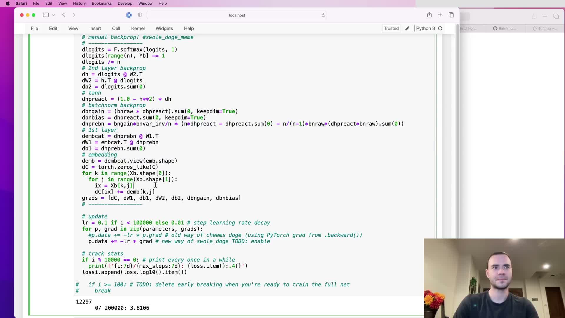
Assembling the previously derived manual gradients—analytic cross-entropy, linear-layer matrix derivatives, tanh nonlinearity, batch-normalization closed-form gradient, embedding lookup accumulation—produces a full backward pass that computes parameter gradients without calling loss.backward.
When parameter updates use these manually computed gradients inside a torch.no_grad block, the training loop behaves equivalently to autograd-based training up to floating-point tolerances; small numerical differences on the order of 1e-9 are typical.
This end-to-end implementation verifies correctness by comparing per-parameter gradients to autograd, then proceeds to update weights and biases, calibrate running BN statistics, evaluate losses, and sample from the model.
Manual implementation provides full transparency into gradient flow and is a valuable debugging and educational tool, even though autograd remains the practical choice for day-to-day development.
Enjoy Reading This Article?
Here are some more articles you might like to read next: