Karpathy Series - Bulding Makemore Part 5 - Wavenet
- Lecture goal: transition from shallow MLP to deeper hierarchical WaveNet-like architecture
- Starter code and dataset overview: reuse of part-three code and dataset statistics
- Modular layer-building approach and API design (linear, batchnorm, 10h)
- Model construction, parameter initialization, and early evaluation behavior
- Smoothing noisy loss plots by reshaping and averaging training trace
- Encapsulating embedding lookup and flattening as explicit layer modules
- Introducing a Sequential container to compose layers and simplify forward pass
- BatchNorm training/evaluation state pitfalls demonstrated by single-example forward
- Baseline performance and rationale for larger context windows
- Empirical improvement from naive scaling of context length to 8 characters
- Tensor shape inspection through the forward pass and multi-dimensional linear multiplication
- Design concept for hierarchical progressive fusion of consecutive tokens
- Flatten_consecutive operator: implementation choices and correctness by view vs explicit concatenation
- Applying flatten_consecutive with n=2 to create a hierarchical model and inspecting activations
- Choosing channel widths to match parameter budgets and initial experiment results
- Diagnosing incorrect BatchNorm statistics when input tensors are three-dimensional
- API divergence from PyTorch’s BatchNorm1d and deliberate channel ordering choice
- Retraining after BatchNorm fix and modest validation improvement
- Scaling embedding dimensionality and hidden units yields further validation gains (crossing 2.0)
- Convolutional interpretation, efficiency via sliding filters, and future work directions
Lecture goal: transition from shallow MLP to deeper hierarchical WaveNet-like architecture
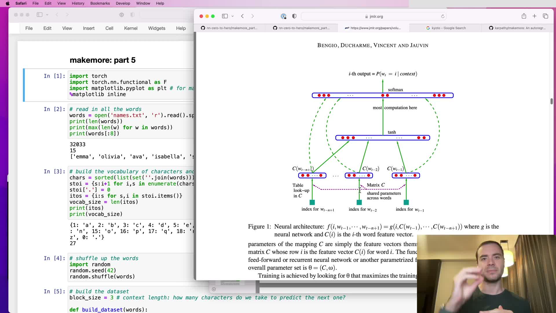
This segment introduces the lecture objective: extend a previously implemented character-level multi-layer perceptron (MLP) into a deeper model that consumes longer contexts and progressively fuses input information, arriving at an architecture conceptually equivalent to WaveNet.
Key reframing of the task:
- Move from a model that conditions on the previous 3 characters to one that accepts a longer context.
- Shift the fusion strategy from compressing all context into a single hidden layer to fusing information across depth (hierarchical, staged fusion).
- Preserve the autoregressive next-character prediction formulation while increasing the receptive field and better retaining temporal structure.
Intended outcome: a hierarchical progressive-fusion network that supports larger receptive fields without destroying stepwise temporal information.
Starter code and dataset overview: reuse of part-three code and dataset statistics
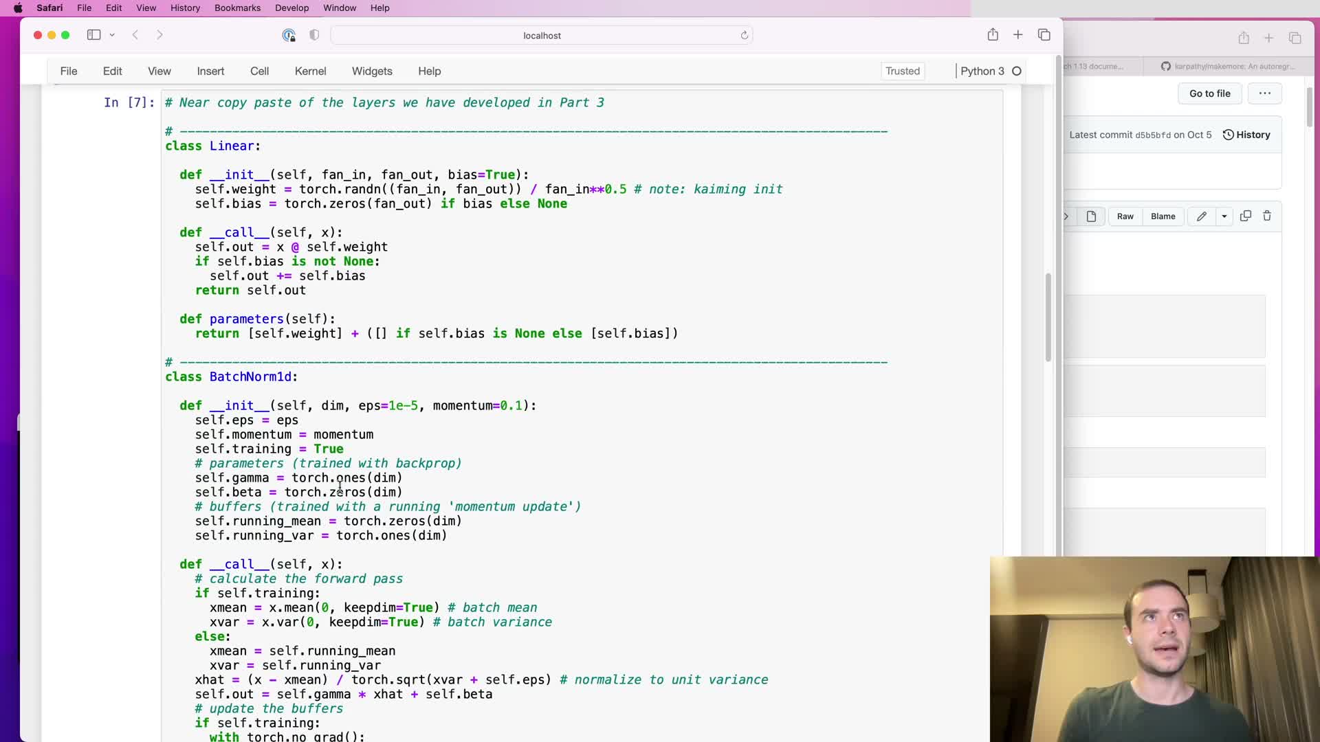
This segment summarizes the starter code provenance and dataset:
- The codebase is largely copied from earlier parts; the data generation pipeline is unchanged.
- Task formulation remains next-character prediction from a short preceding context.
- Dataset size and form: roughly 182,000 examples for the 3→1 task (preprocessing and example generation unchanged).
Why this matters:
- Establishes a familiar baseline environment (same training loop and data loader).
- Architectural experiments will operate on this unchanged data pipeline so observed effects come from model changes rather than data quirks.
Modular layer-building approach and API design (linear, batchnorm, 10h)
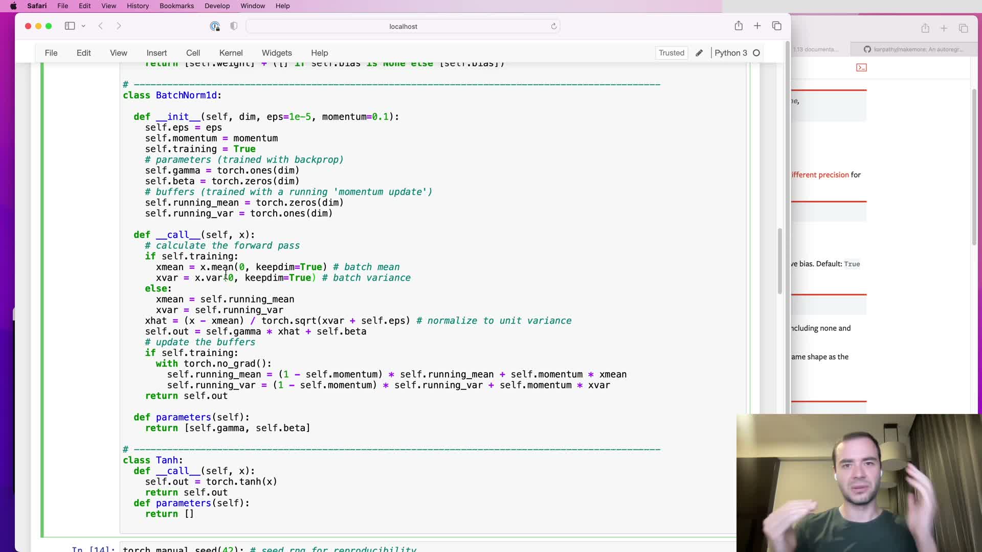
This segment explains the decision to implement neural network components as modular layer classes with APIs modeled after PyTorch’s torch.nn:
- Implement basic building blocks as Lego-style modules (e.g., Linear, BatchNorm1d equivalents, and an elementwise nonlinearity like ‘10h’).
- Keep forward signatures familiar so these modules can be swapped with real PyTorch components later.
Why this design:
- Makes modules composable into larger graphs.
- Eases readability, testing, and later replacement with official libraries.
BatchNorm-like layer caveats:
- Has external state (running mean and variance).
- Behavior depends on training vs. evaluation mode (per-batch stats vs. running stats).
- Introduces cross-example coupling, so mode mismanagement can cause subtle, hard-to-find bugs (e.g., bad variance estimates, NaNs).
Model construction, parameter initialization, and early evaluation behavior
This segment covers assembling the initial network:
- Architecture: an embedding table followed by a sequence of Linear → BatchNorm → nonlinearity → Linear.
- Use weight scaling at initialization to avoid excessively large initial logits.
- Expose parameters so standard gradient-based optimizers can operate.
Practical notes:
- Initial parameter count was on the order of ~12k.
- Optimizer and loss setup follow standard practice (e.g., SGD/Adam + cross-entropy for next-char prediction).
- Observed issue: high-variance loss estimates caused by very small batch sizes.
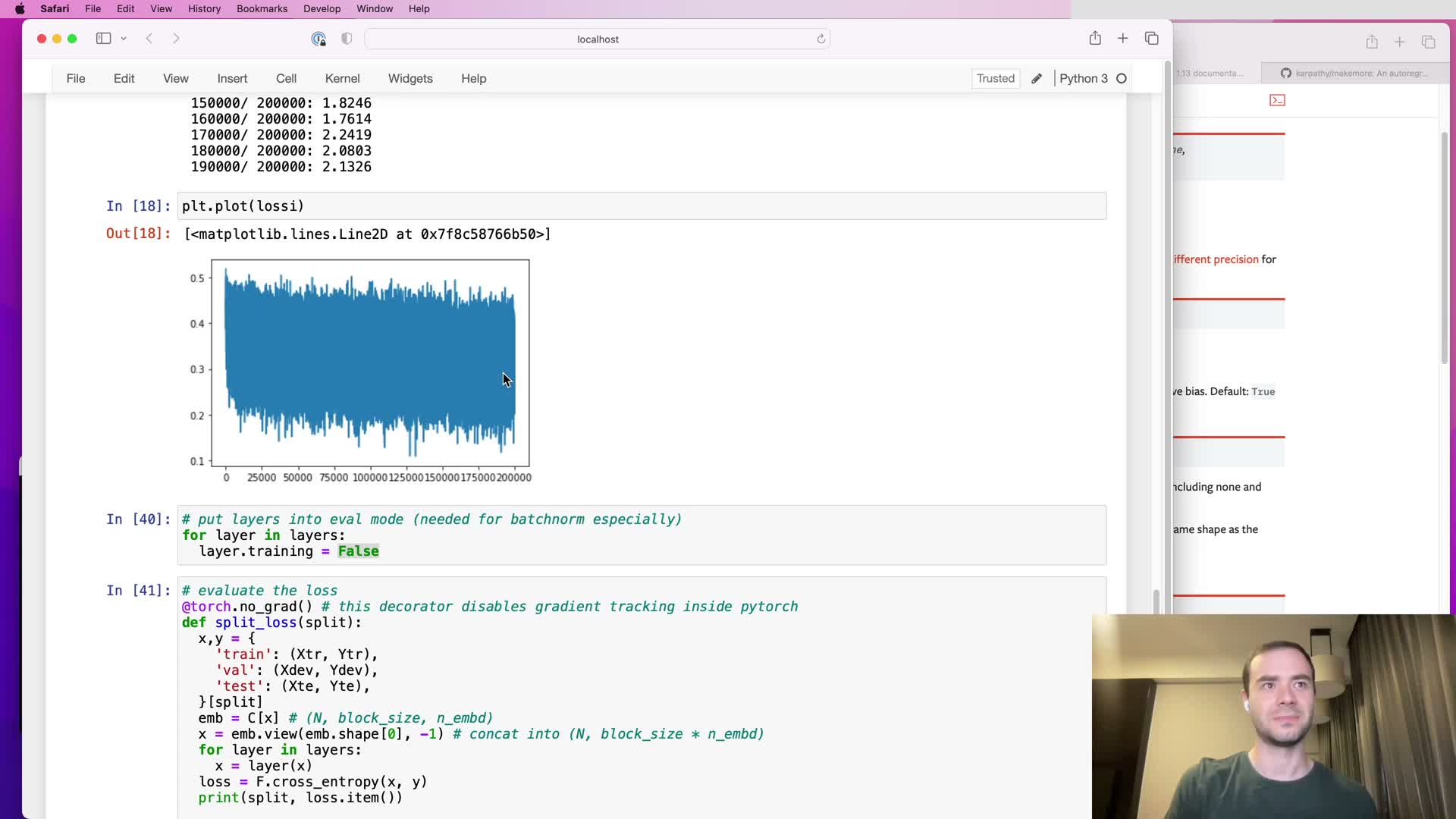
- Important evaluation procedure for models with BatchNorm: set training=False (eval mode) so the model uses running statistics for stable validation and sampling.
Smoothing noisy loss plots by reshaping and averaging training trace
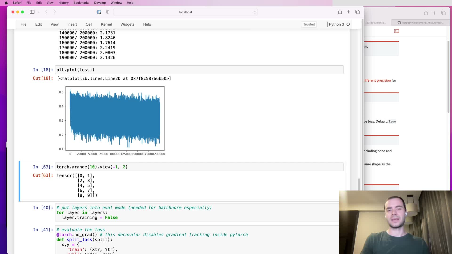
This segment describes a simple technique to de-noise the logged scalar training trace:
- Reshape a 1-D list of loss values into a 2-D tensor with rows of a chosen length (e.g., 1000), then compute the mean along rows to produce a smoothed sequence for plotting.
- Use PyTorch’s view/reshape semantics and the -1 placeholder to compute chunk-wise statistics efficiently without copying memory.
Why do this:
- Smooths noisy scalar traces so learning curves are easier to interpret.
- Makes it simpler to visualize effects like learning rate decay, plateaus, or sudden instabilities.
Encapsulating embedding lookup and flattening as explicit layer modules
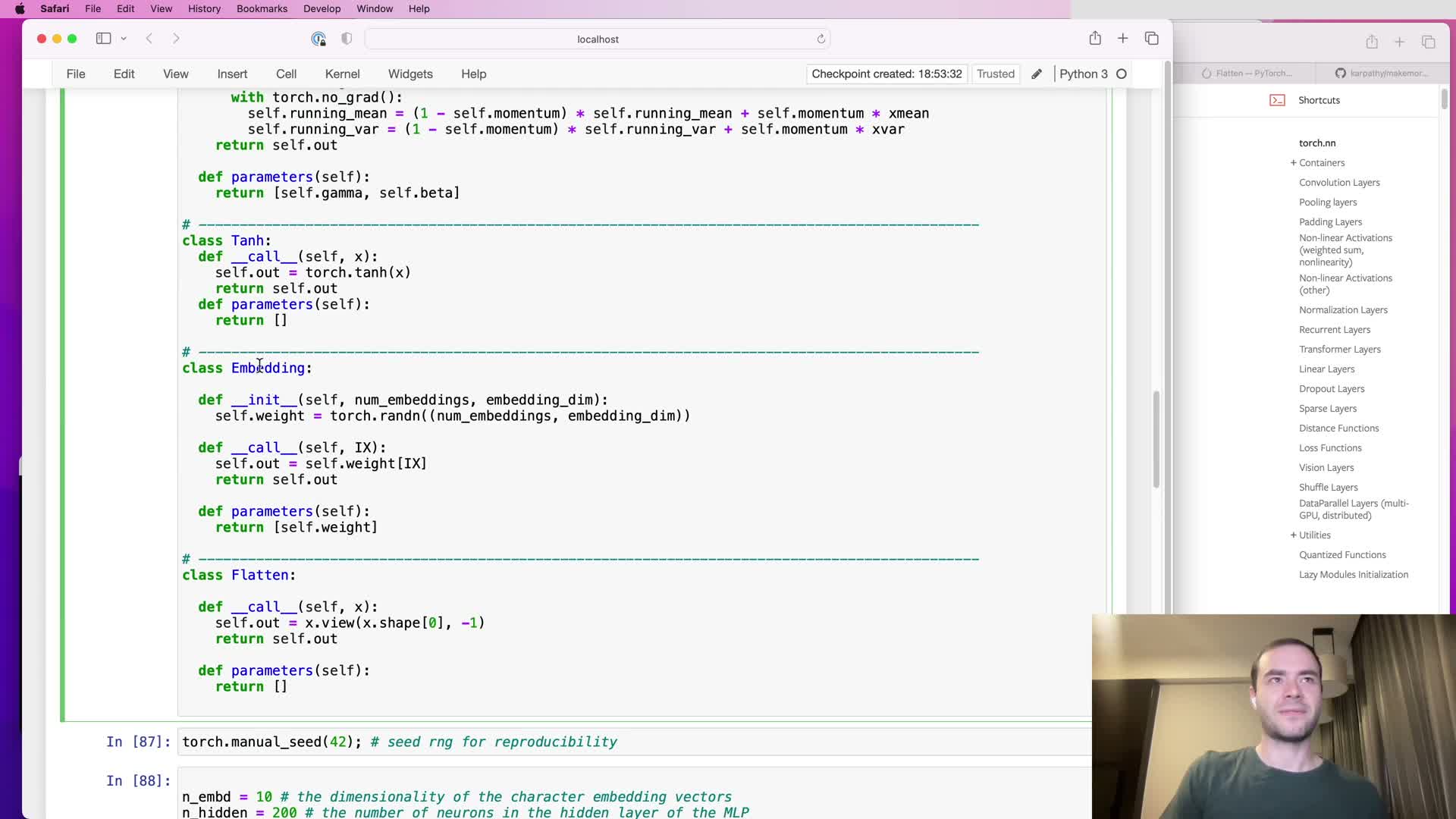
This segment explains refactoring special-case operations into first-class module classes:
- Move embedding table indexing into an Embedding module that mirrors torch.nn.Embedding: exposes the weight matrix and implements index-based lookup in forward.
- Move view-based flattening into a Flatten module that performs reshape/view without copying memory.
Advantages:
- Uniform model definition: the entire network becomes a homogeneous sequence of modules.
- Simplifies forward logic and parameter management (parameters and buffers are exposed consistently).
Introducing a Sequential container to compose layers and simplify forward pass
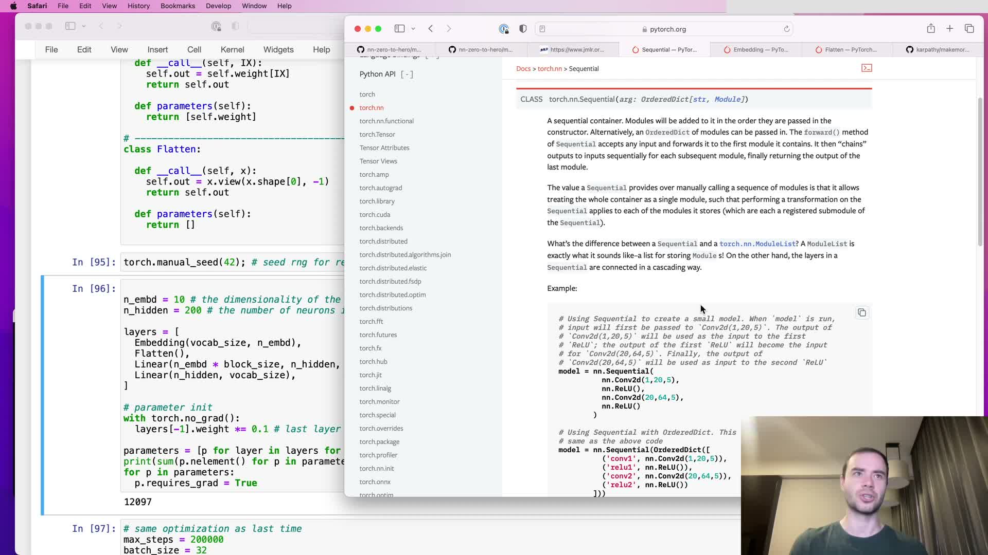
This segment introduces a Sequential container module that aggregates child modules:
- The container holds an ordered list of child modules and implements a forward pass that pipes input through each child sequentially.
- Responsibilities:
- Maintain child modules in order.
- Expose aggregated parameters and buffers.
- Provide a single callable object so the model can be invoked as model(x).
- Maintain child modules in order.
Result:
- Substantial simplification of training and sampling code.
- Cleaner modularity and clearer parameter extraction for optimizers.
BatchNorm training/evaluation state pitfalls demonstrated by single-example forward
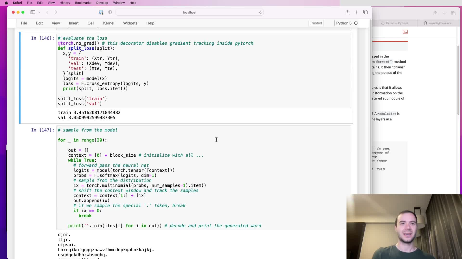
This segment demonstrates a typical bug caused by misusing BatchNorm:
- Symptom: forwarding a single-example batch while BatchNorm is left in training mode yields invalid variance estimates (variance over a single scalar is zero/undefined), which can propagate NaNs through the network.
- Mechanism: BatchNorm maintains running mean/variance updated by an exponential moving average (EMA) during training, but inference should use those running statistics rather than per-batch estimates.
Takeaway: explicitly toggle module mode (train() vs eval()) when switching between training, validation, and sampling to avoid catastrophic numerical issues.
Baseline performance and rationale for larger context windows
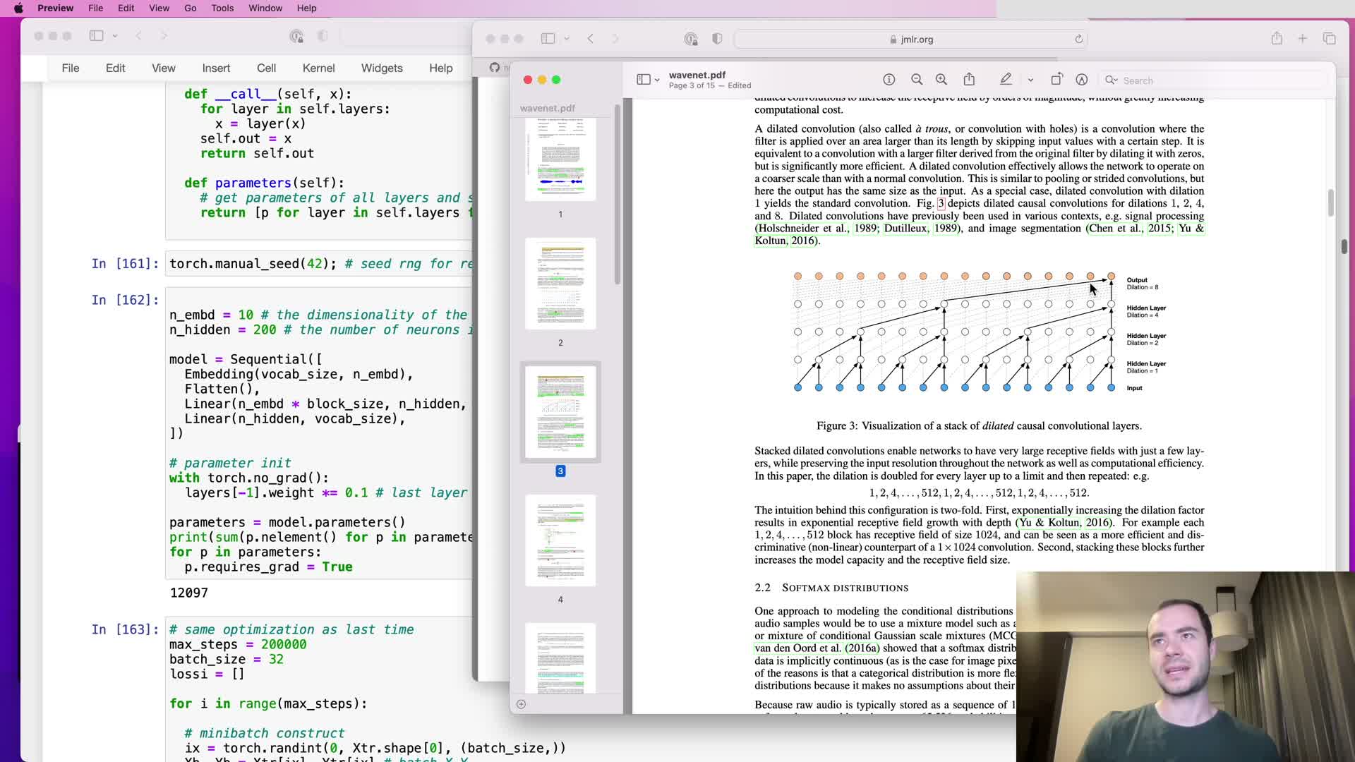
This segment reports baseline loss numbers after fixes and motivates increasing context window:
- Baseline numbers after initial fixes: training loss ≈ 2.05, validation loss ≈ 2.10.
- Observation: similar training and validation loss suggests limited overfitting, which points to capacity or receptive field limitations rather than data scarcity.
Motivation: increase the block size from 3 → 8 characters to give the model a larger context to condition on and thereby capture longer-range dependencies.
Empirical improvement from naive scaling of context length to 8 characters
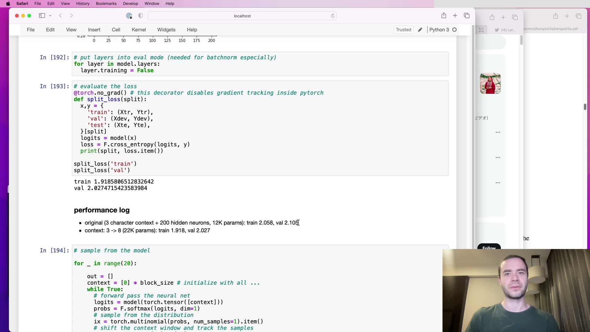
This segment reports the empirical effect of increasing block size from 3 to 8 while keeping a flattened MLP-style architecture:
- Validation loss improved from ~2.10 → ~2.02.
- Sampled outputs became qualitatively more name-like, indicating better sequence modeling.
Interpretation:
- Larger receptive field helps, establishing a useful baseline.
- Caveat: naive scaling of input length into a flat MLP is not the most principled way to distribute parameters — better gains may be available from architecture-aware designs.
Tensor shape inspection through the forward pass and multi-dimensional linear multiplication
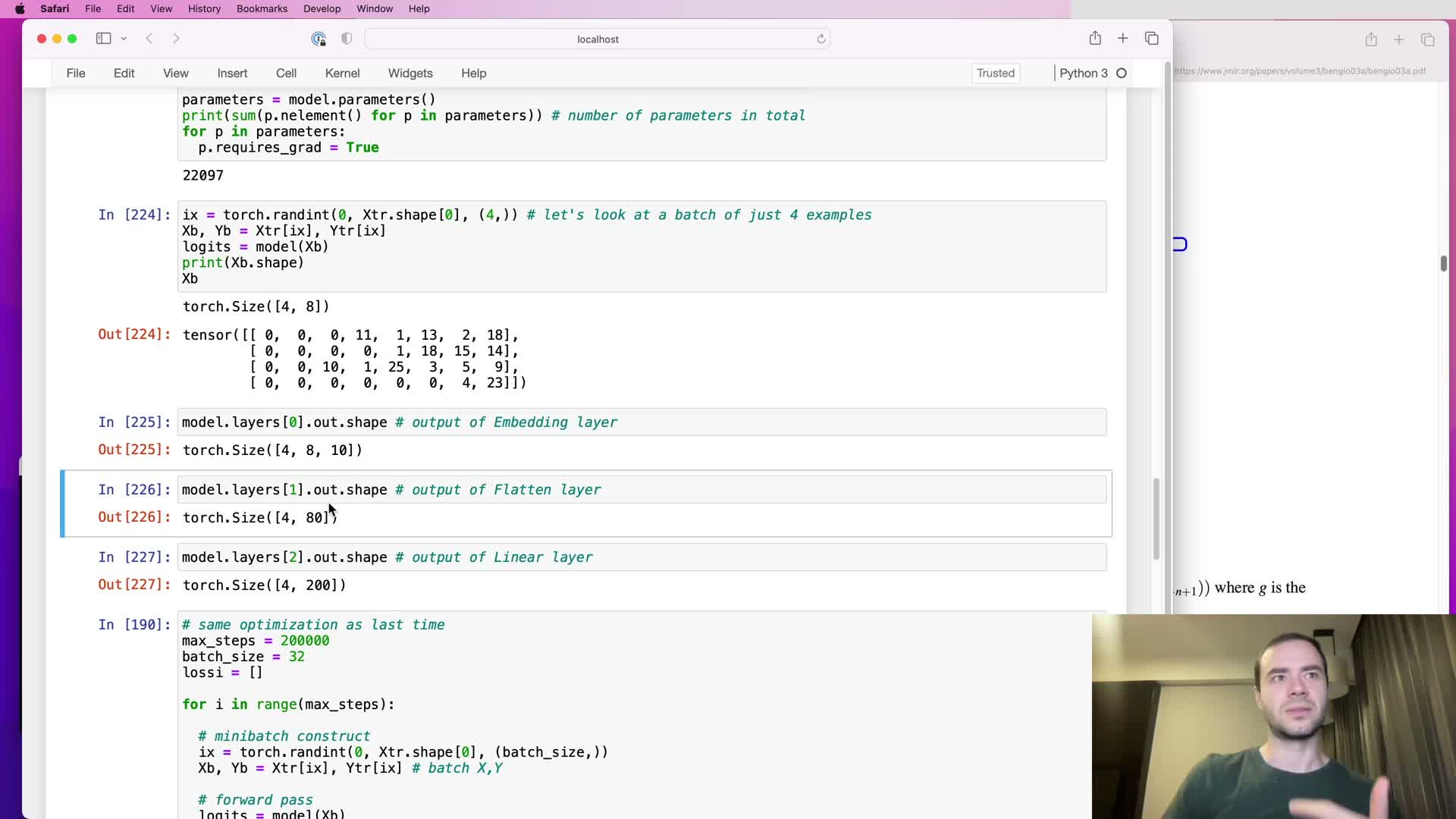
This segment inspects intermediate tensor shapes to validate behavior:
- Confirmed shapes:
- Embedding output: B × T × C.
- Flattening: B × (T*C).
- Linear layer: matrix multiply behaves as expected, with bias broadcasting applied.
- Embedding output: B × T × C.
- Important PyTorch feature: Linear layers accept inputs with extra leading batch dimensions (e.g., B × X × D) and perform the matrix multiply across the last dimension, producing outputs with corresponding leading dimensions (B × X × D_out).
Why this matters:
- Treating grouped elements as extra batch-like dimensions enables parallel processing of groups and is central to the hierarchical fusion design.
Design concept for hierarchical progressive fusion of consecutive tokens
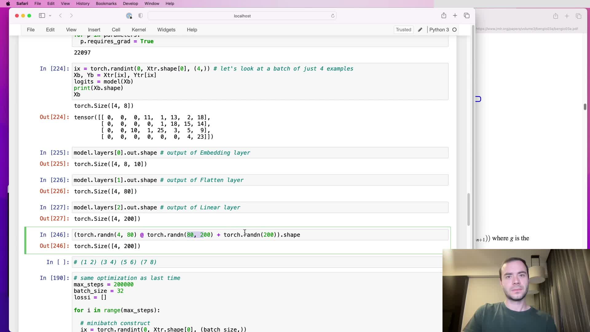
This segment presents the hierarchical fusion strategy:
- Instead of flattening all token embeddings into one long vector, group consecutive tokens (e.g., bigrams), flatten per-group, apply the same projection across groups in parallel, then repeat fusion hierarchically so each layer doubles the effective receptive field.
- Example shape progression (B=4, T=8, C=10):
- 4 × 8 × 10 → (group pairs) → 4 × 4 × 20 → 4 × 2 × 40 → …
- 4 × 8 × 10 → (group pairs) → 4 × 4 × 20 → 4 × 2 × 40 → …
Key points:
- Grouping introduces an extra batch-like dimension so groups can be processed in parallel.
- Rationale: progressive aggregation avoids crushing all context in one step and mirrors the tree-like receptive field expansion used in WaveNet-style architectures.
Flatten_consecutive operator: implementation choices and correctness by view vs explicit concatenation
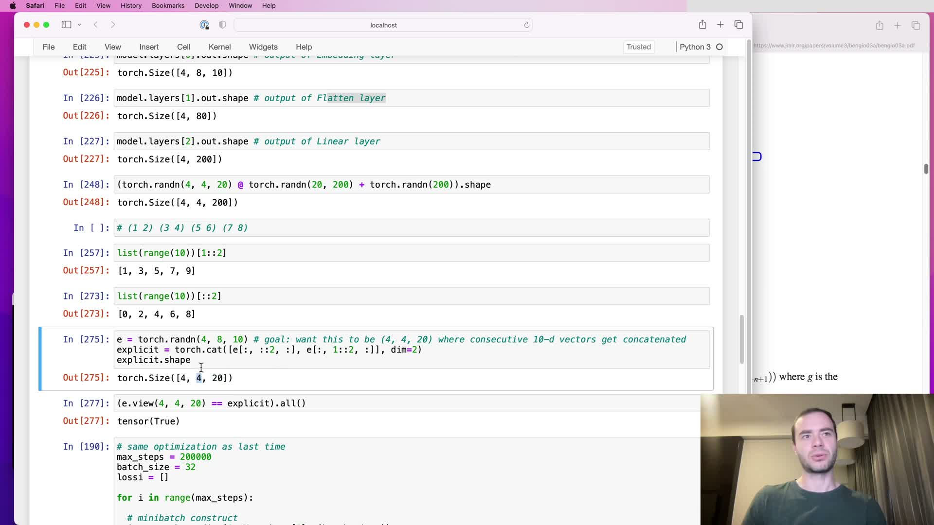
This segment details the implementation of a FlattenConsecutive module:
- Purpose: fuse n consecutive time steps into the last dimension by reshaping B × T × C → B × (T//n) × (C*n).
- Two implementation approaches:
- Explicit slicing and concatenation of even/odd indices (more code, more indexing).
- Use view/reshape with correctly computed target dimensions and integer division for group counts (compact and zero-copy when layout allows).
- Explicit slicing and concatenation of even/odd indices (more code, more indexing).
Edge cases and design choices:
- When the grouped time dimension reduces to 1, consider squeezing spurious singleton dimensions so the module preserves prior 2‑D behavior when n == T.
Applying flatten_consecutive with n=2 to create a hierarchical model and inspecting activations
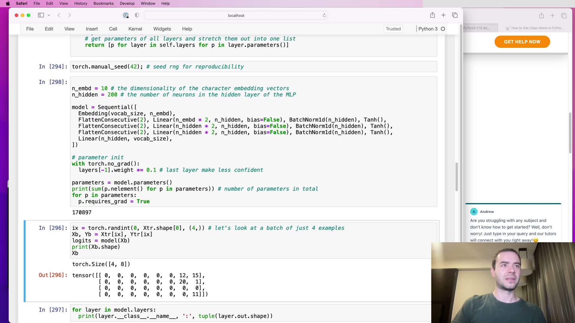
This segment implements the hierarchical model using FlattenConsecutive(n=2):
- Replace the original single-step flatten with FlattenConsecutive(n=2) and stack Linear → BatchNorm → Nonlinearity blocks that expect the smaller per-group input dimensionality (C*n).
- Verified forward propagation with shape printing: BatchNorm, elementwise nonlinearities, and subsequent projections work with 3-D tensors because they operate across the last dimension and broadcast over leading batch-like dimensions.
Result: the network computes the same final logits as before but performs staged fusion across depth, corresponding to a single branch of a tree-like WaveNet receptive field.
Choosing channel widths to match parameter budgets and initial experiment results
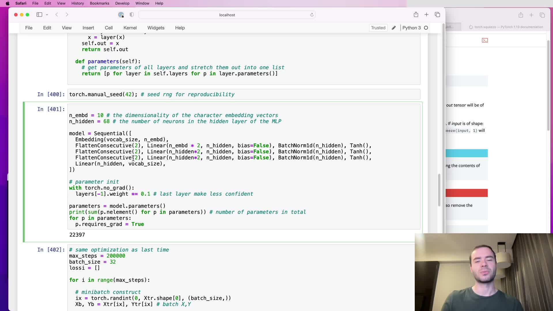
This segment discusses matching parameter budgets for fair comparison:
- Choose hidden dimensionalities (e.g., hidden = 68) so the hierarchical network matches the previous flat network’s parameter count (~22k).
- With this matched budget, the initial hierarchical design produced validation loss very close to the flat baseline (~2.029 vs ~2.027).
Takeaway: architectural change alone did not yet yield a clear gain; how channels are allocated across layers remains an important hyperparameter to explore.
Diagnosing incorrect BatchNorm statistics when input tensors are three-dimensional
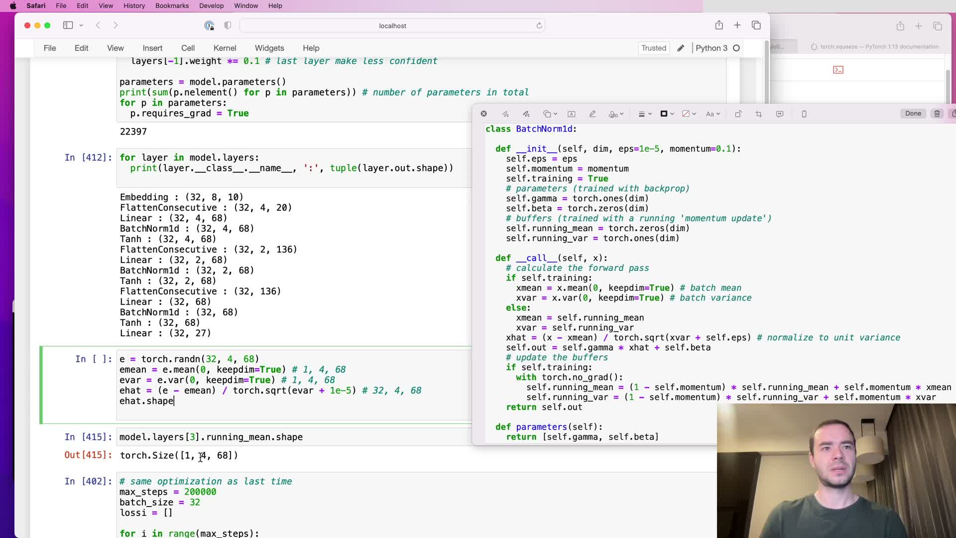
This segment diagnoses a subtle BatchNorm bug introduced by the 3-D inputs:
- Bug: BatchNorm computed mean/variance only over the zeroth dimension when inputs became 3-D (B × G × C), producing running mean shapes like 1 × G × C and treating each group position independently.
- Correct behavior: reduce over both sample and group dimensions so per-channel statistics aggregate across the composite batch.
- Technical fix: use torch.mean with a tuple of dimensions (e.g., (0,1) for 3-D inputs) instead of only (0,), and select (0,) for 2-D inputs.
Rationale: pooling over both batch and group dimensions increases the effective sample size for statistics and yields more stable running mean/variance estimates.
API divergence from PyTorch’s BatchNorm1d and deliberate channel ordering choice
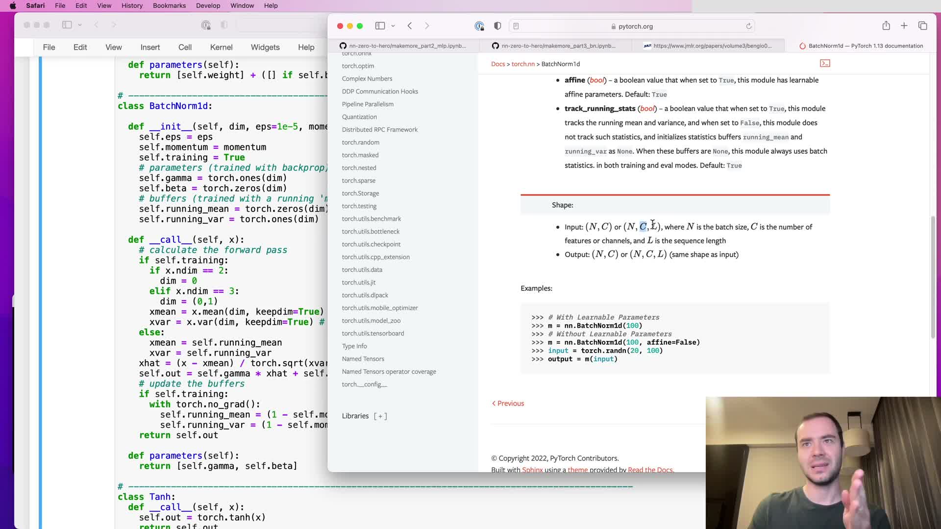
This segment explains how the custom BatchNorm1d differs from PyTorch’s API and why:
- PyTorch convention: inputs shaped N × C or N × C × L (channels in the middle).
- Custom implementation: uses N × L × C (channels last) and treats leading dimensions as batch-like for the hierarchical pipeline.
- Implication for reductions:
- PyTorch’s default reduction for 3-D is over (0,2) (collapse sample and temporal dims, keep channels).
- Custom needs to reduce over (0,1) to aggregate sample and group dims when channels are last.
- PyTorch’s default reduction for 3-D is over (0,2) (collapse sample and temporal dims, keep channels).
Justification: the channels-last layout simplifies hierarchical processing where groups appear as extra leading dimensions. The correctness of the change can be validated by inspecting the running mean shape (expected 1 × 1 × C after the fix).
Retraining after BatchNorm fix and modest validation improvement
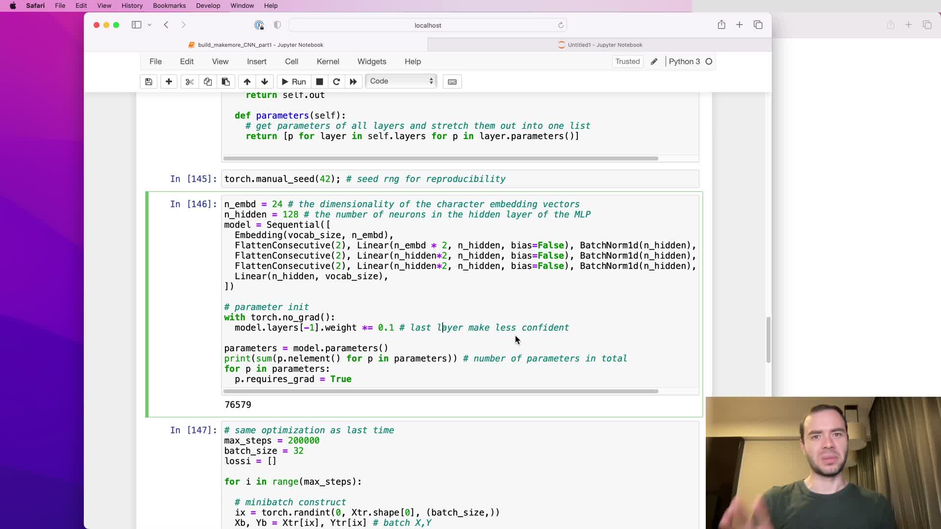
This segment reports retraining after fixing BatchNorm reduction behavior:
- Observed small validation improvement (e.g., ~2.029 → ~2.022).
- Why improvement is expected:
- Pooling statistics across both sample and group dimensions yields more stable mean and variance estimates.
- Improved stability in normalization leads to slightly better numerical stability and optimization.
- Pooling statistics across both sample and group dimensions yields more stable mean and variance estimates.
Caveat: the improvement is modest and may not be statistically significant, but it validates the correctness of BatchNorm behavior with multi-dimensional inputs.
Scaling embedding dimensionality and hidden units yields further validation gains (crossing 2.0)
This segment covers scaling experiments and tradeoffs:
- Scaling: increasing embedding size from 10 → 24 and enlarging hidden units increased model capacity to roughly ~76k parameters.
- Result: noticeable validation improvement to below 2.0 (about 1.993).
Tradeoffs and practicalities:
- Larger models generally improve performance but need longer training and more careful hyperparameter tuning.
- Current workflow lacks an automated experimental harness to efficiently explore learning rates, regularization, and channel allocation.
Conclusion: promising preliminary results that invite systematic, automated exploration.
Convolutional interpretation, efficiency via sliding filters, and future work directions

This concluding segment connects the hierarchical linear blocks to convolutional implementations and outlines next steps:
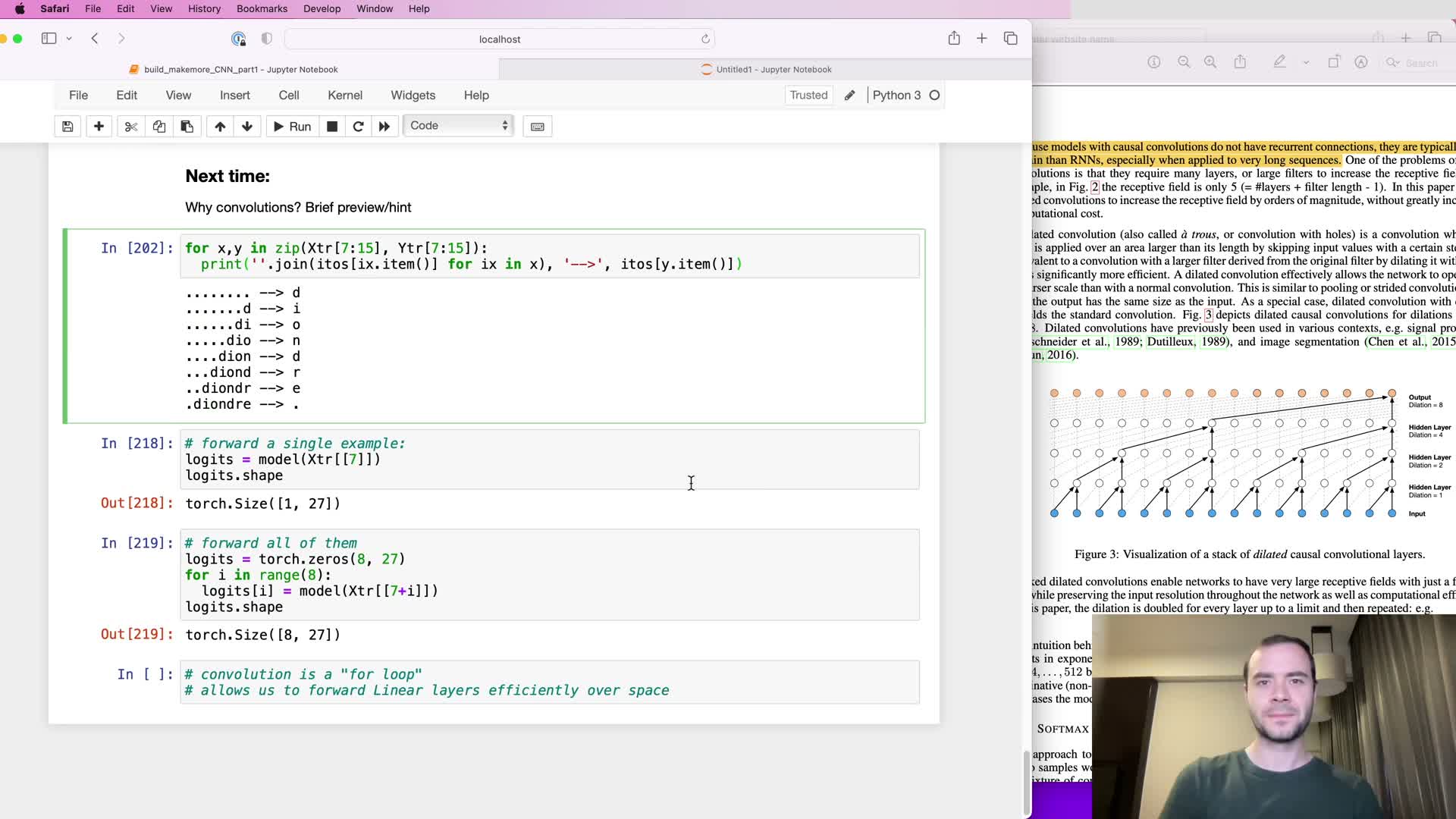
- Conceptual equivalence: the hierarchical linear blocks compute a single computational tree per output. Dilated causal convolutions implement the same mapping more efficiently by sliding shared filters across inputs and reusing intermediate computations.
- Why convolutions are an implementation optimization (not a modeling change):
- They hide Python-level loops inside highly optimized kernels.
- They reuse intermediate values instead of recomputing overlapping subtrees.
- They allow computing many outputs in parallel with shared weights.
- They hide Python-level loops inside highly optimized kernels.
Next steps suggested:
- Implement dilated causal convolutions to realize the tree-like receptive field efficiently.
- Add gated linear units (GLUs), residual, and skip connections following the WaveNet design.
- Set up an experimental harness for systematic hyperparameter search (learning rates, regularization, channel allocations).
- Explore other sequence models (e.g., RNNs, Transformers) for comparison and additional insights.
Enjoy Reading This Article?
Here are some more articles you might like to read next: