Karpathy Series - Let's build GPT from scratch
- ChatGPT demonstrates probabilistic sequence completion.
- The Transformer architecture underlies modern autoregressive language models like GPT.
- A minimal educational goal is to train a character-level Transformer on a small dataset.
- NanoGPT is a minimal codebase that reproduces Transformer training behavior.
- Load and inspect the training corpus in a reproducible environment.
- Construct the character vocabulary and determine the vocabulary size.
- Tokenization design trades vocabulary size for sequence length.
- Encode the entire dataset as a contiguous integer tensor.
- Split data into training and validation subsets and define block size for contexts.
- Each sampled chunk contains multiple training examples via shifted inputs and targets.
- Train the model to handle contexts ranging from single token up to block size during inference.
- Batching stacks multiple independent chunks for parallel processing.
- The simplest language model is a bigram model implemented via token embeddings.
- Compute cross-entropy loss by reshaping logits and targets to match framework expectations.
- Implement autoregressive generation by sampling from softmaxed logits at the last time step.
- Initialize and optimize the model with Adam, then run a standard training loop.
- Initial training of the bigram model reduces loss but cannot capture long-range context.
- Package the notebook code into a script with device handling and stable loss estimation.
- Self-attention can be approximated as weighted aggregation of past token vectors, initially illustrated by cumulative averaging.
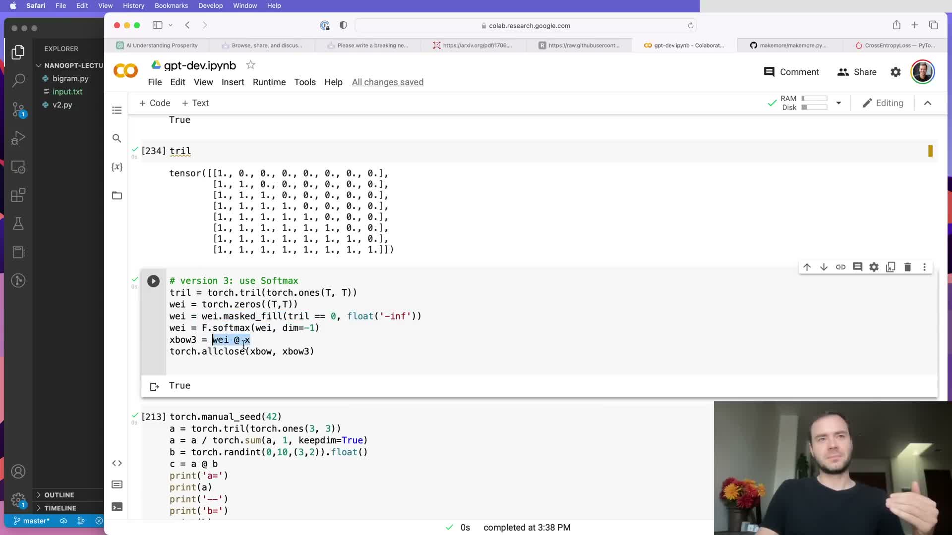
- Lower-triangular weight matrices and batched matrix multiplication vectorize prefix aggregation.
- Masking with negative infinity and softmax produces normalized, causal affinity weights.
- Introduce embeddings and an output projection to separate token identity and model dimensionality.
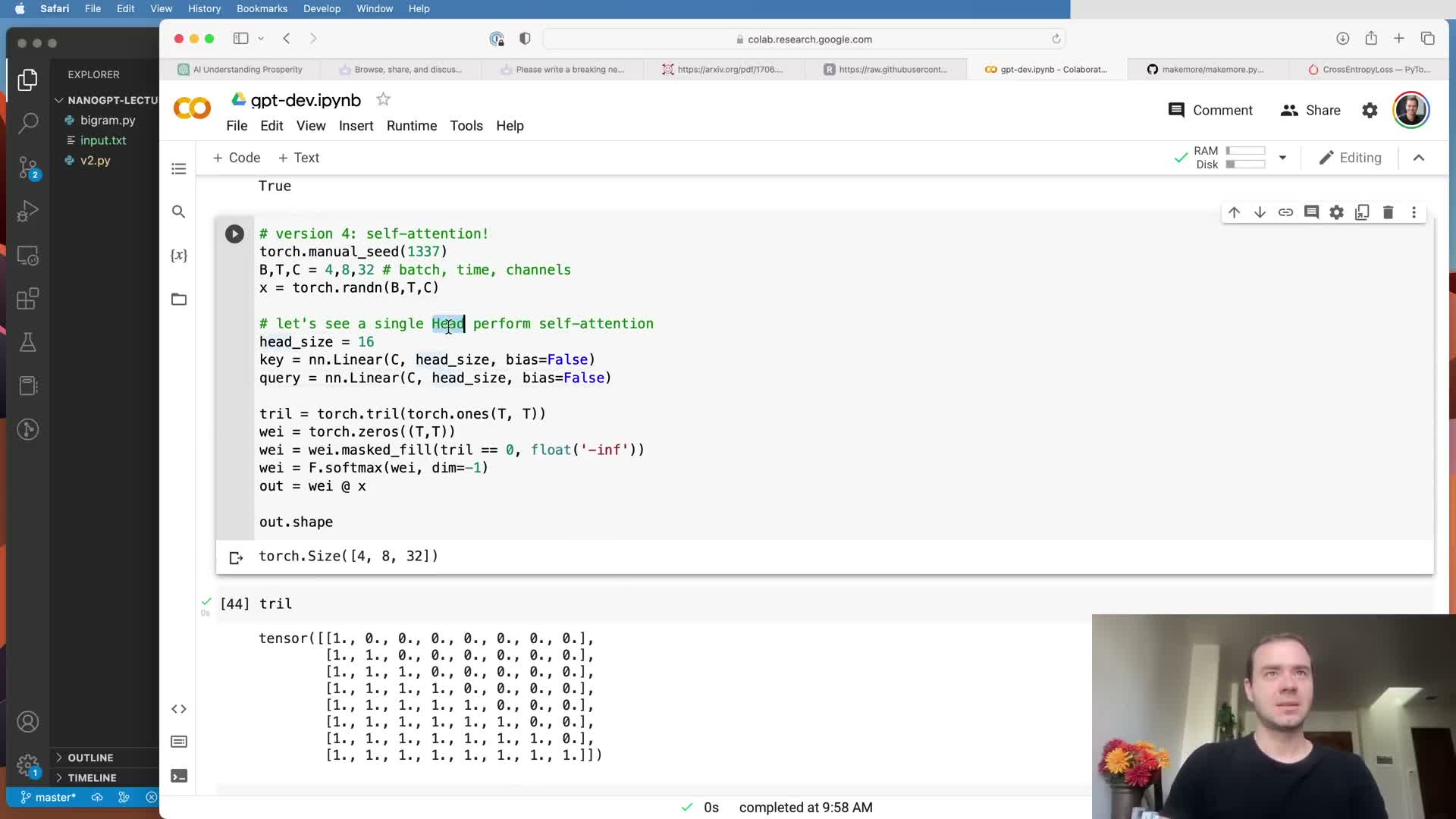
- Self-attention computes data-dependent affinities via query-key dot products and aggregates values accordingly.
- Attention is a general communication mechanism with graph and positional considerations.
- Scale dot-product attention by 1/sqrt(d_k) to control variance and softmax sharpness.
- Implement a single self-attention head module and integrate it into the model while enforcing context cropping.
- Training with a single scaled attention head yields modest gains, while multi-head attention improves representation capacity.
- Add a per-position feed-forward network to allow tokens to process gathered context independently.
- Stack Transformer blocks with residual projections to enable deep architectures.
- Use feed-forward inner expansion and LayerNorm (pre-norm) to stabilize training.
- Add dropout and scale up model hyperparameters to improve generalization and capacity.
- A decoder-only Transformer implements autoregressive language modeling; encoder-decoder variants support conditioned sequence-to-sequence tasks.
- Large-scale models require pre-training on massive corpora then fine-tuning and alignment to become useful assistants.
- NanoGPT implementation details and summary of the educational reproduction.
ChatGPT demonstrates probabilistic sequence completion.

A conversational AI like ChatGPT implements a language model that generates text by sequentially completing a given input sequence.
The model produces token-by-token outputs in a probabilistic manner, so the same prompt can yield different plausible continuations on different runs.
Key points:
-
Tokens can be words, subwords, or characters.
-
The model estimates conditional probabilities of the next token given prior context: P(next_token previous_tokens).
- This inherent probabilistic completion behavior is the foundation for prompt engineering, creative generation, and sampling variability.
The Transformer architecture underlies modern autoregressive language models like GPT.

The Transformer, introduced in “Attention Is All You Need” (2017), is the core sequence model used in GPT-style systems.
Highlights:
- It replaced recurrence with attention mechanisms that compute data-dependent interactions across sequence positions.
- This enables scalable parallel computation across time steps instead of sequential recurrence.
-
GPT = Generative Pre-trained Transformer: a Transformer pre-trained on large corpora and then adapted for downstream tasks.
- The architecture began in machine translation but became the foundation for many large-scale language models with relatively minor modifications.
A minimal educational goal is to train a character-level Transformer on a small dataset.

A compact, instructive variant of GPT can be trained on a toy corpus such as tiny Shakespeare (Shakespeare’s works concatenated into a small text file).
Why this is useful:
- Training a character-level model simplifies tokenization and implementation while preserving the pedagogical value of sequence modeling and attention.
- The model predicts the next character conditioned on preceding characters and, after training, can generate arbitrary-length text in the training corpus’ style.
- This setup demonstrates core concepts of autoregressive generation without requiring massive compute or internet-scale data.
NanoGPT is a minimal codebase that reproduces Transformer training behavior.

NanoGPT is a compact GitHub repository that implements Transformer training with very small code (two main files), illustrating the essential components required to reproduce known baselines.
Notable aspects:
- Shows that a correct implementation plus modest compute can replicate smaller released models (e.g., GPT-2 small) on standard datasets.
- Separates model definition from the training script, and includes utilities for loading pretrained weights.
- Demonstrates real-world engineering practices in a simplified form with an instructional goal: develop the model from scratch in a notebook for clarity.
Load and inspect the training corpus in a reproducible environment.
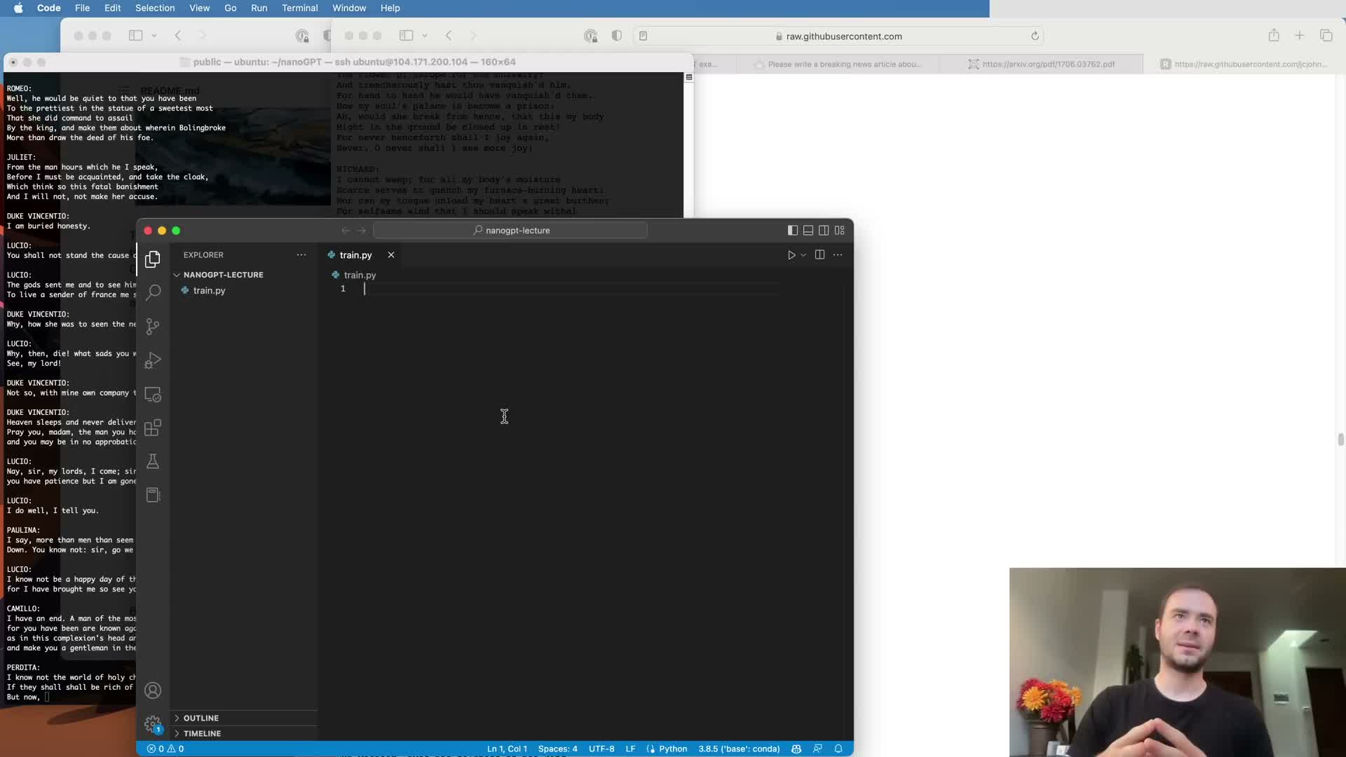
Begin experiments in a shareable environment such as a Google Colab notebook:
- Download the tiny Shakespeare corpus and load it as a single string for processing.
- Confirm dataset size and inspect initial characters to validate data integrity and encoding assumptions.
- Use the notebook to enable step-by-step development, reproducibility, and sharing of the training workflow and artifacts.
This initial validation helps catch I/O and encoding issues before further modeling steps.
Construct the character vocabulary and determine the vocabulary size.
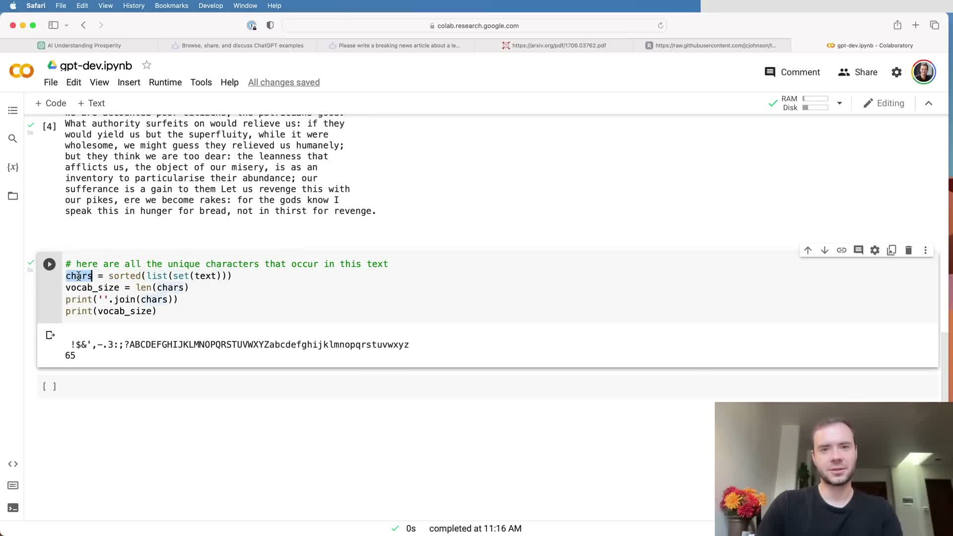
Extract the set of unique characters in the corpus and sort them to obtain a stable vocabulary ordering.
Key consequences:
-
Vocabulary size = number of unique tokens the model will consider (e.g., ~65 characters for tiny Shakespeare, including whitespace and punctuation).
- The vocabulary defines the model’s output dimensionality and the size of the embedding table.
- Character-level vocabularies are compact but produce longer sequences; establish a deterministic char→int mapping for encoding/decoding model I/O.
Tokenization design trades vocabulary size for sequence length.
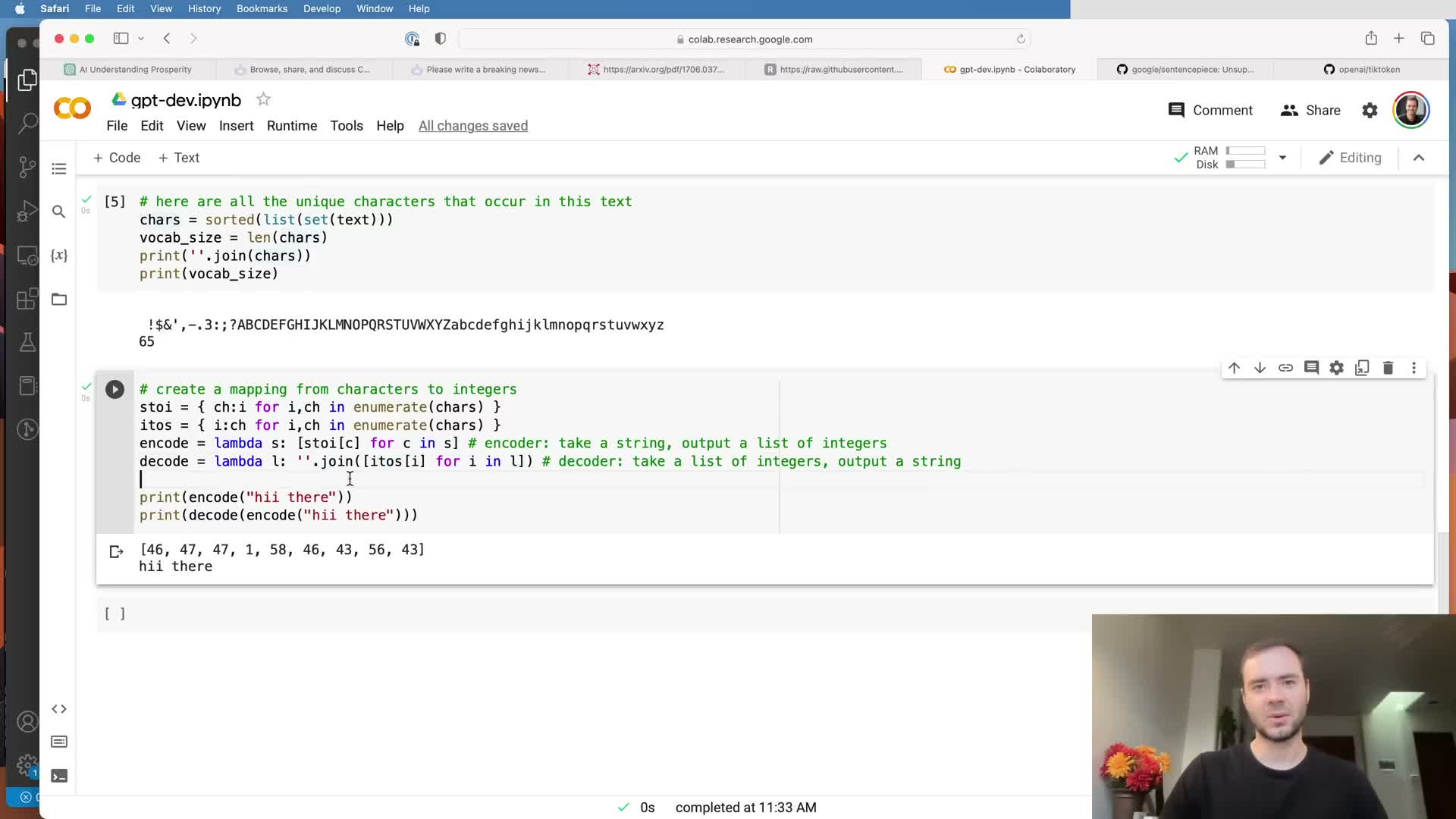
Tokenization converts raw text into integer sequences according to a vocabulary schema.
Options and trade-offs:
-
Character-level tokenizers: tiny vocabulary, simple mapping, longer sequences — preferred for instructional clarity.
-
Subword tokenizers (e.g., SentencePiece, Byte-Pair Encoding): larger vocabularies (tens of thousands), shorter sequences — used in practical large-scale models.
- The tokenizer choice determines embedding table size, tokenization/de-tokenization logic, and batching behavior.
Encode the entire dataset as a contiguous integer tensor.
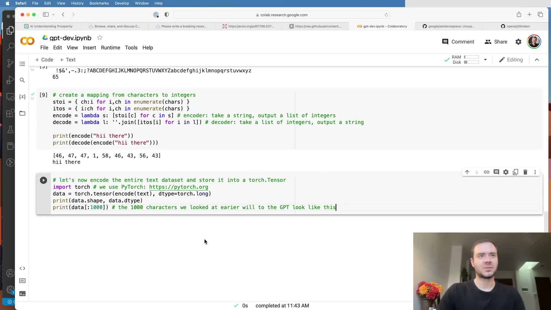
After defining encoder and decoder mappings, translate the whole corpus into a single long integer sequence and wrap it into a framework tensor (e.g., a PyTorch tensor) to serve as the data array.
Benefits and checks:
- Contiguous representation simplifies sampling random chunks for training and splitting into train/validation segments.
- Storing the dataset as a tensor facilitates efficient slicing and batching during mini-batch construction.
- Confirm correctness by inspecting correspondence between text slices and integer slices.
Split data into training and validation subsets and define block size for contexts.

Partition the data tensor into a training portion (e.g., first 90%) and a held-out validation portion (last 10%) to monitor generalization and detect overfitting.
Workflow and definitions:
- Define a maximum context length commonly called block_size or context length.
- Training samples are randomly extracted contiguous chunks of length block_size (with a target offset), not the entire corpus at once.
- Working with chunks reduces memory/compute requirements and enables the model to learn dependencies across shorter contexts.
- Keep the validation split hidden during training as an unbiased generalization estimate.
Each sampled chunk contains multiple training examples via shifted inputs and targets.
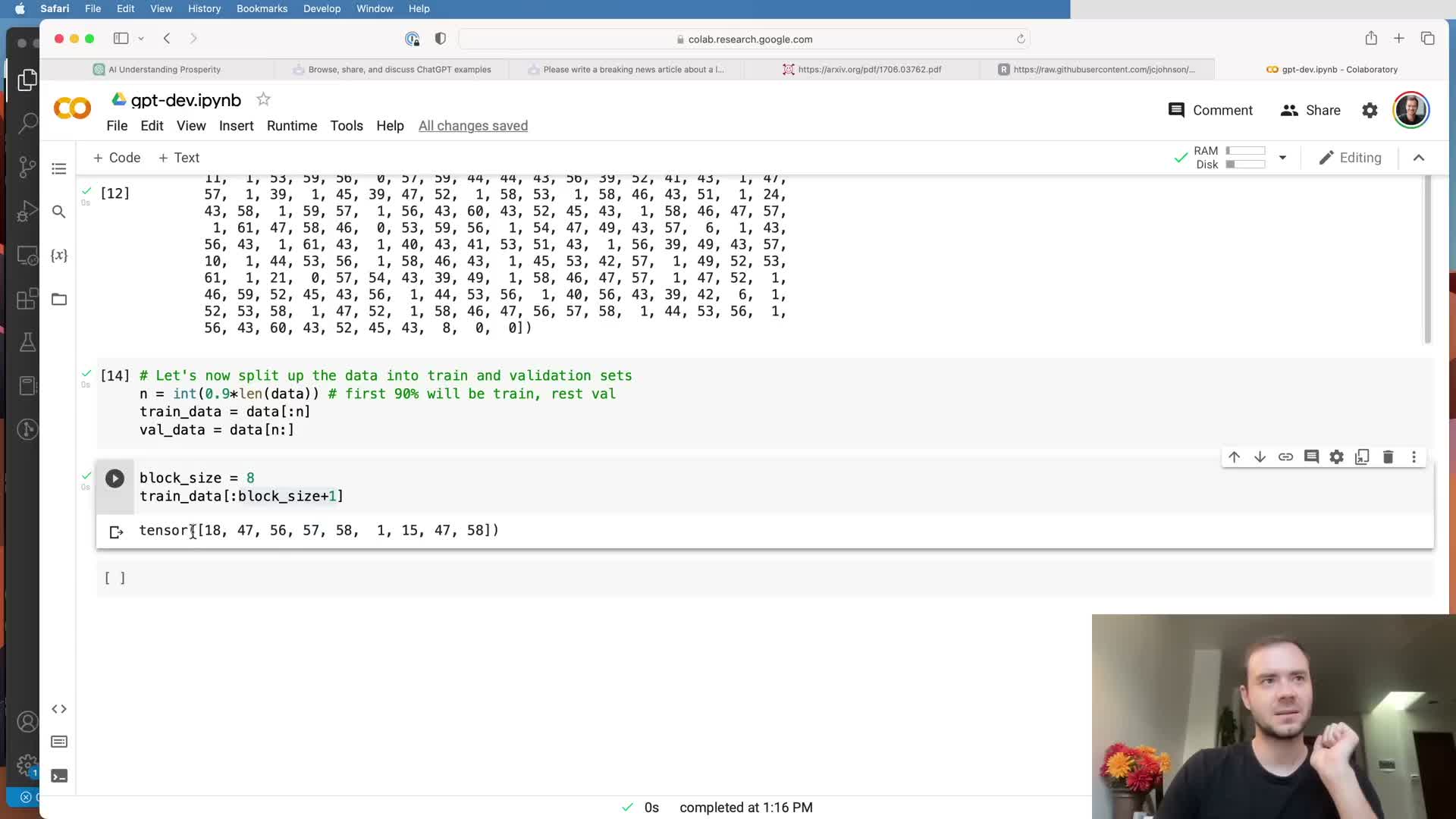
When extracting a chunk of length block_size + 1 from the sequence, construct inputs and targets as follows:
- Inputs X = the first block_size tokens of the chunk.
- Targets Y = the following tokens offset by one (the next token for each input position).
- This packs block_size training examples (one per time position) into each chunk and lets the model learn to predict the next token from all prefix lengths up to the block size.
The offset-by-one construction is fundamental to autoregressive next-token prediction.
Train the model to handle contexts ranging from single token up to block size during inference.
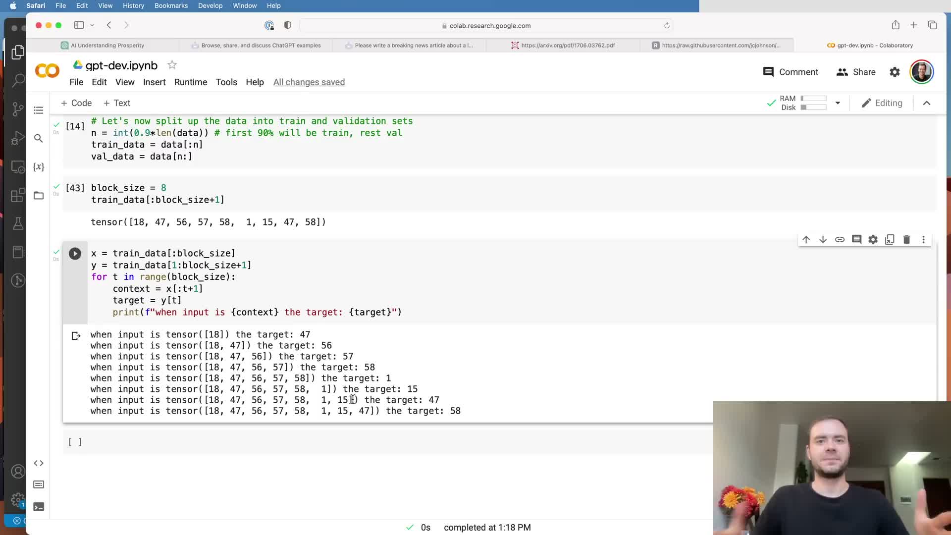
Include examples with context lengths from 1 up to block_size during training to condition the model on short and long contexts.
Implications:
- This is critical for sampling, where generation often begins with a minimal prompt and the context progressively grows.
- The model must generalize to intermediate context sizes during autoregressive sampling; longer-than-block_size contexts must be truncated.
- Truncation is necessary because positional embeddings are defined up to block_size.
Batching stacks multiple independent chunks for parallel processing.
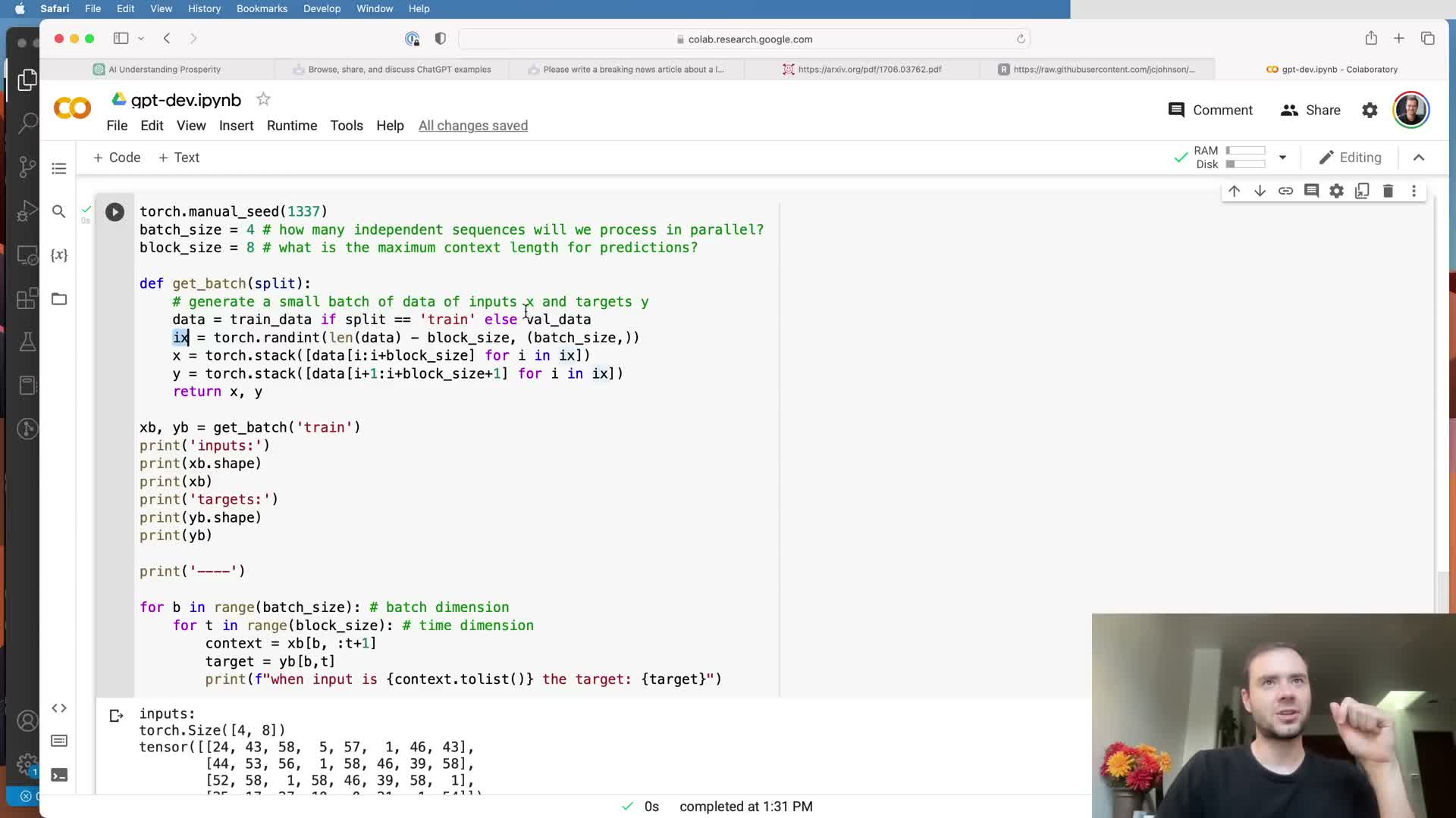
Add a batch dimension by sampling multiple random chunk offsets to create a batch of independent sequences and stack these into a tensor of shape (batch_size, block_size) for efficient parallel processing on accelerators.
Practical notes:
- Batching keeps hardware utilization high and enables parallel gradient computation across independent examples (batches do not exchange information).
- Use randomized extraction of chunk offsets and a reproducible RNG seed for deterministic experiment replication.
- Batched targets are handled analogously and later flattened for loss computation to match expected shapes.
The simplest language model is a bigram model implemented via token embeddings.
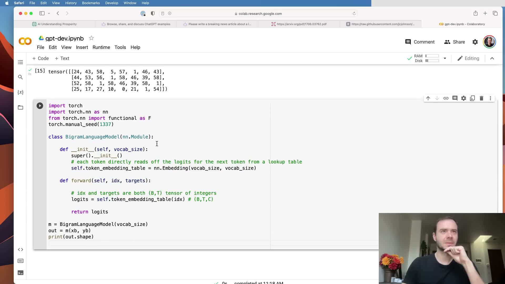
A bigram model predicts the next token solely from the identity of the current token using a token embedding table that is directly interpreted as logits for the next-token distribution.
Implementation and role:
- In PyTorch: an nn.Embedding shaped (vocab_size, vocab_size) so each token index indexes a row that scores all possible next tokens.
- The bigram model ignores context beyond the current token but can capture local correlations (some tokens strongly predict specific followers).
- Use this simple model as a baseline and a clean starting point before adding contextual mechanisms like attention.
Compute cross-entropy loss by reshaping logits and targets to match framework expectations.
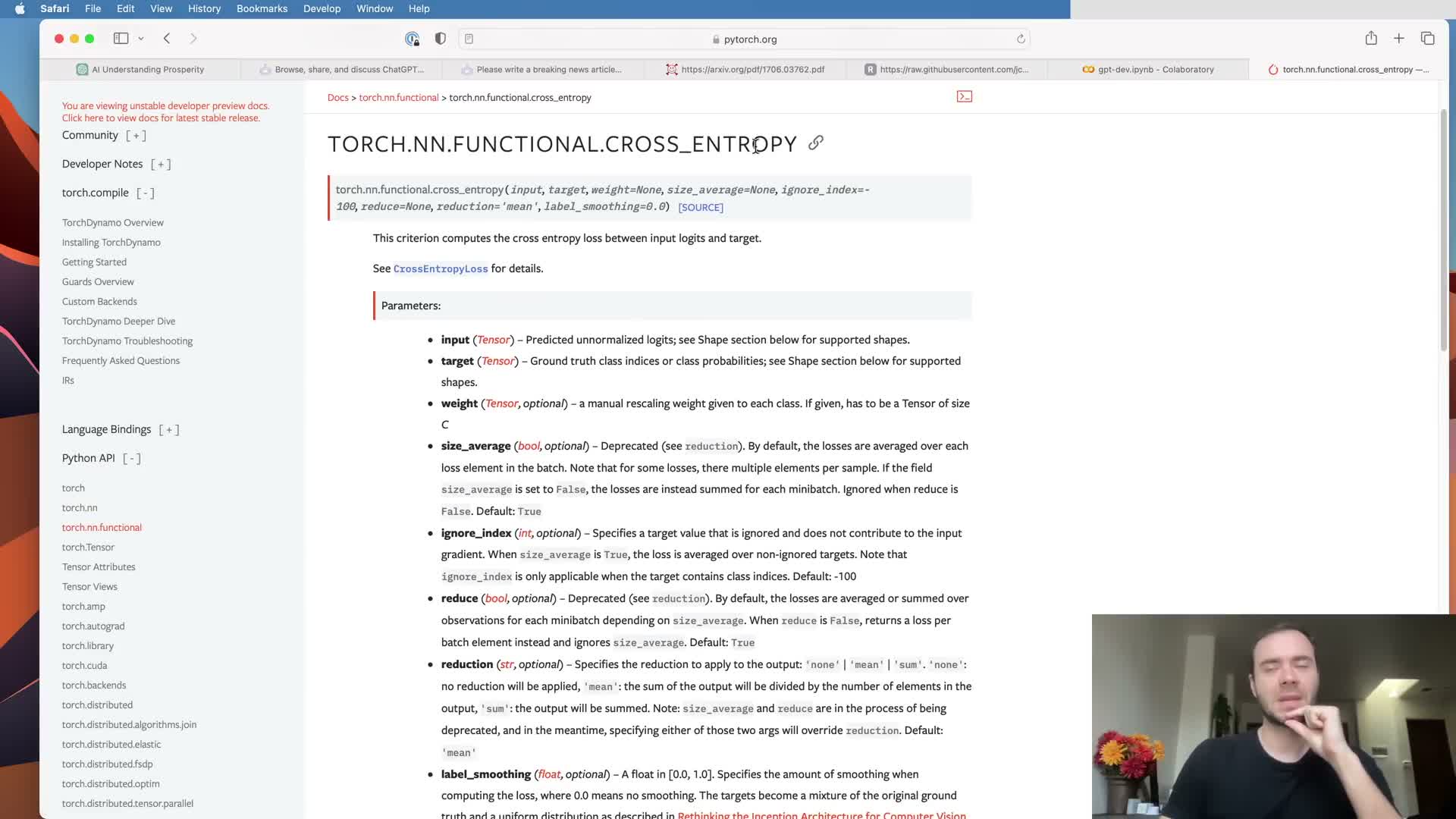
For multi-dimensional logits with shape (B, T, C), frameworks like PyTorch require rearrangement to a two-dimensional shape (BT, C)** before calling cross-entropy; similarly, targets of shape **(B, T)** must be flattened to **(BT,).
Practical checklist:
- Reshape or view tensors so the channel dimension is preserved as the second dimension and batch-time positions become the first flattened dimension.
- This aligns predictions and labels for negative log-likelihood computation and produces a scalar loss measuring next-token predictive quality.
- Sanity-check the initialization by comparing expected random-start loss to -log(1 / vocab_size).
Implement autoregressive generation by sampling from softmaxed logits at the last time step.
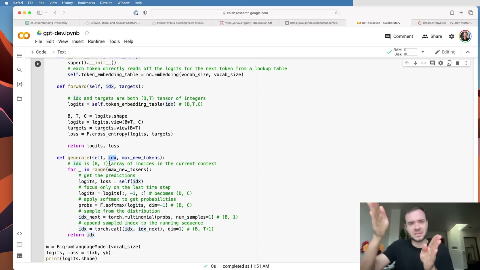
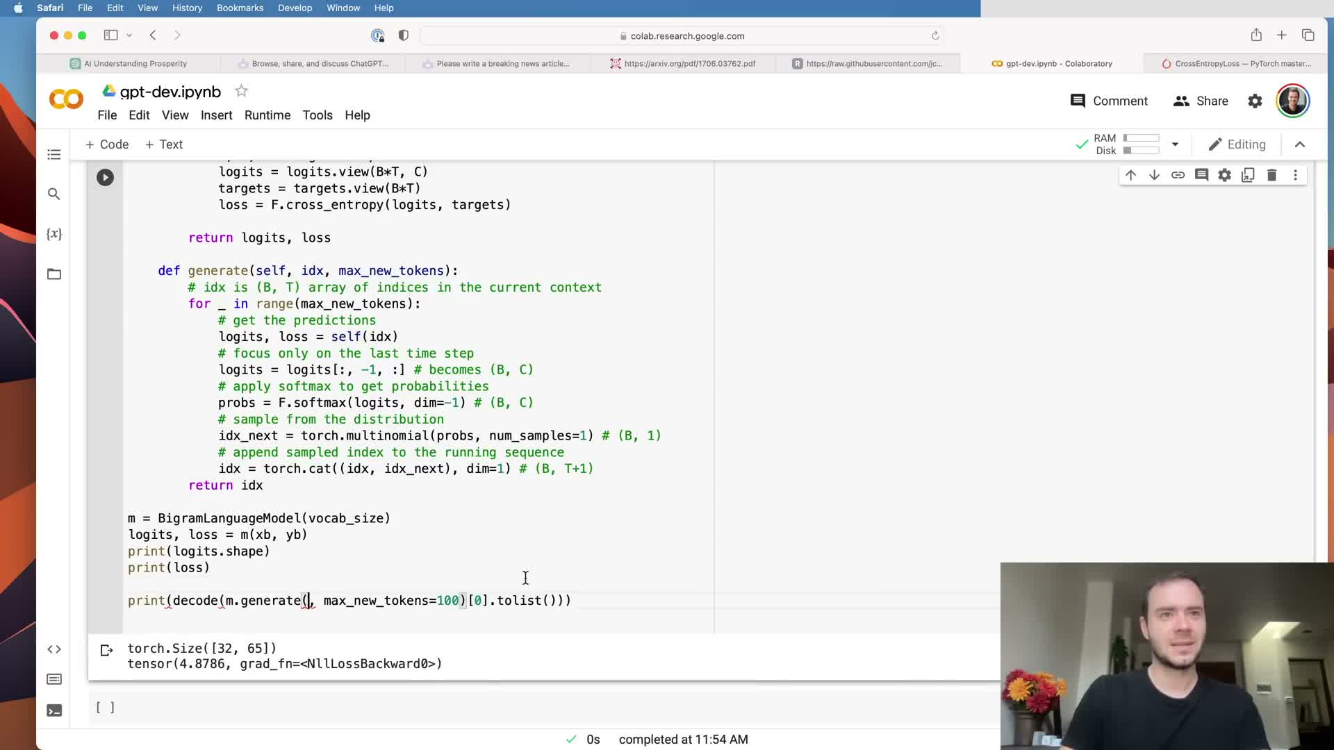
Generation extends an input context by repeatedly calling the model and sampling next tokens.
Canonical generation loop:
- Run the model on the current context and extract logits for the last time step.
- Convert logits to probabilities via softmax.
- Sample the next token with a multinomial draw and append it to the running context.
- Repeat for the desired number of new tokens to produce a variable-length sequence.
Implementation tips:
- Make targets optional in the model forward to support both training (return loss) and generation (return logits).
- Batched generation returns a batch of sequences that can be decoded back to text by mapping token indices to characters/words.
Initialize and optimize the model with Adam, then run a standard training loop.
Create an optimizer such as Adam with a suitable learning rate (e.g., ~3e-4 typical, though small networks may require adjustments) and perform the canonical training loop:
- Sample a batch.
- Compute loss.
- Zero gradients.
- Backpropagate.
- Step the optimizer.
Training practices:
- Monitor loss over many iterations and increase batch size and iteration count when scaling to larger models.
- Use periodic evaluation on the held-out validation split to detect overfitting and tune hyperparameters (learning rate, batch size, etc.).
Initial training of the bigram model reduces loss but cannot capture long-range context.
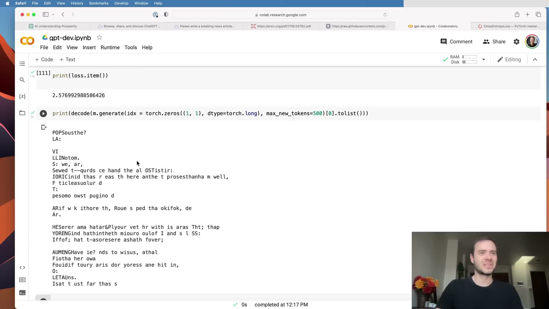
Training the bigram model with gradient-based optimization typically reduces loss from random initialization but remains limited because tokens do not communicate beyond immediate neighbors.
Consequences and motivation:
- Tokens cannot access historical context, so predictions rely only on local correlations.
- Improving next-token prediction requires mechanisms for tokens to access and aggregate relevant information from previous positions—this motivates attention mechanisms.
- The observed loss reduction confirms optimization is working and sets a baseline for architectural improvements.
Package the notebook code into a script with device handling and stable loss estimation.
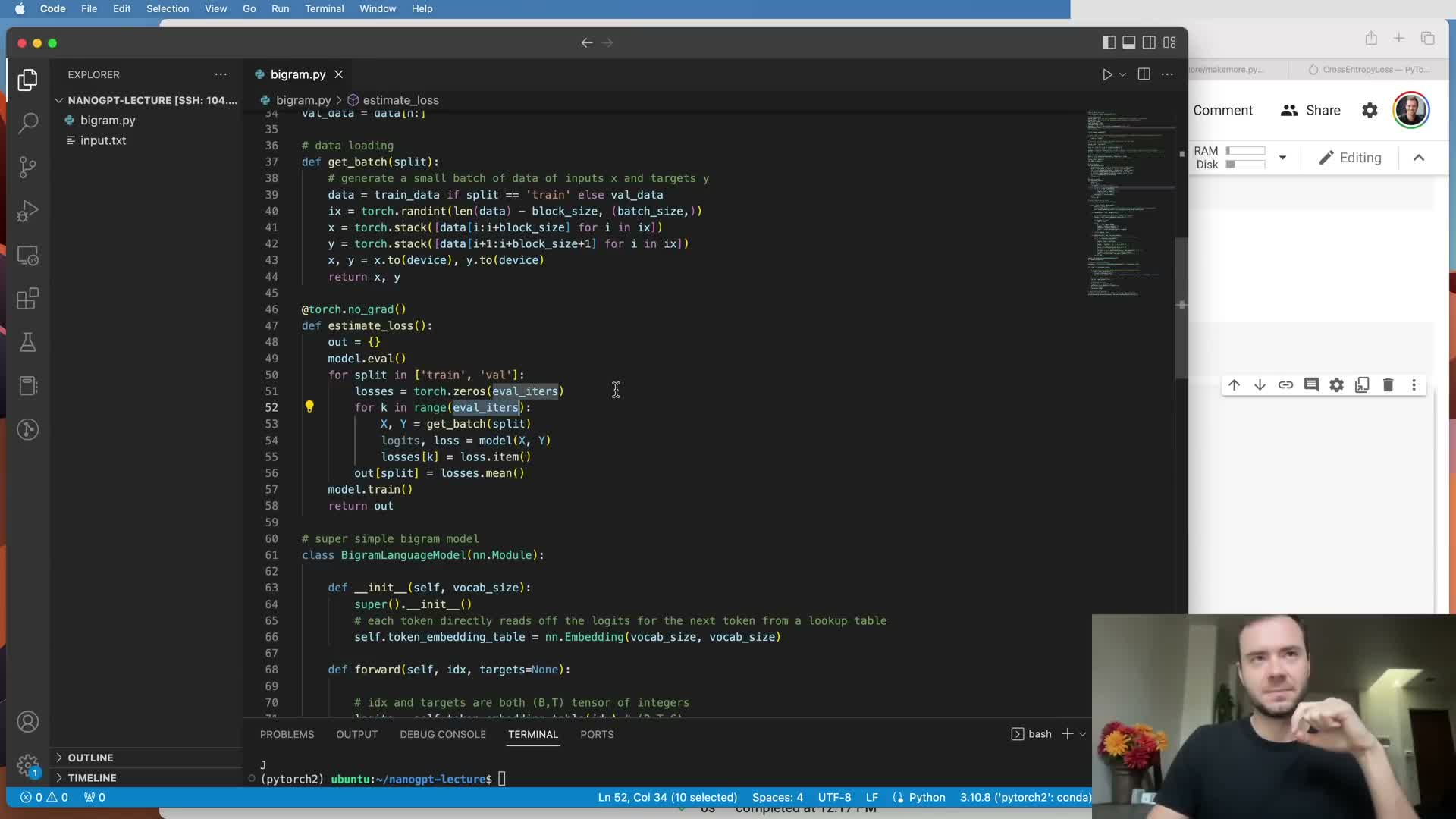
Converting the notebook into a script centralizes hyperparameters, supports running on GPUs by managing device placement, and adds engineering features such as checkpointing and evaluation scheduling.
Suggested engineering additions:
- Add checkpoint saving/loading and device management.
- Implement an estimate_loss routine that averages training and validation loss over several batches to reduce noise.
- Use evaluation mode and torch.no_grad() during validation to avoid gradient computation and reduce memory usage.
These production-oriented changes improve reproducibility and interpretability of training runs.
Self-attention can be approximated as weighted aggregation of past token vectors, initially illustrated by cumulative averaging.
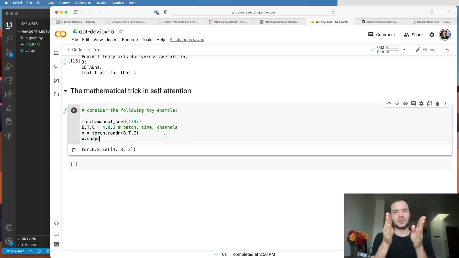
A simple communication mechanism for sequential tokens is to aggregate preceding token vectors by averaging, producing a context summary for each position.
Notes and trade-offs:
- A naive loop implementation is correct but inefficient; it serves as an intuitive toy illustration of past→present information flow.
- This bag-of-words style aggregation demonstrates the goal of attention: fuse information from previous positions into per-token representations.
- The next step is to express such aggregations as batched matrix multiplications for efficiency.
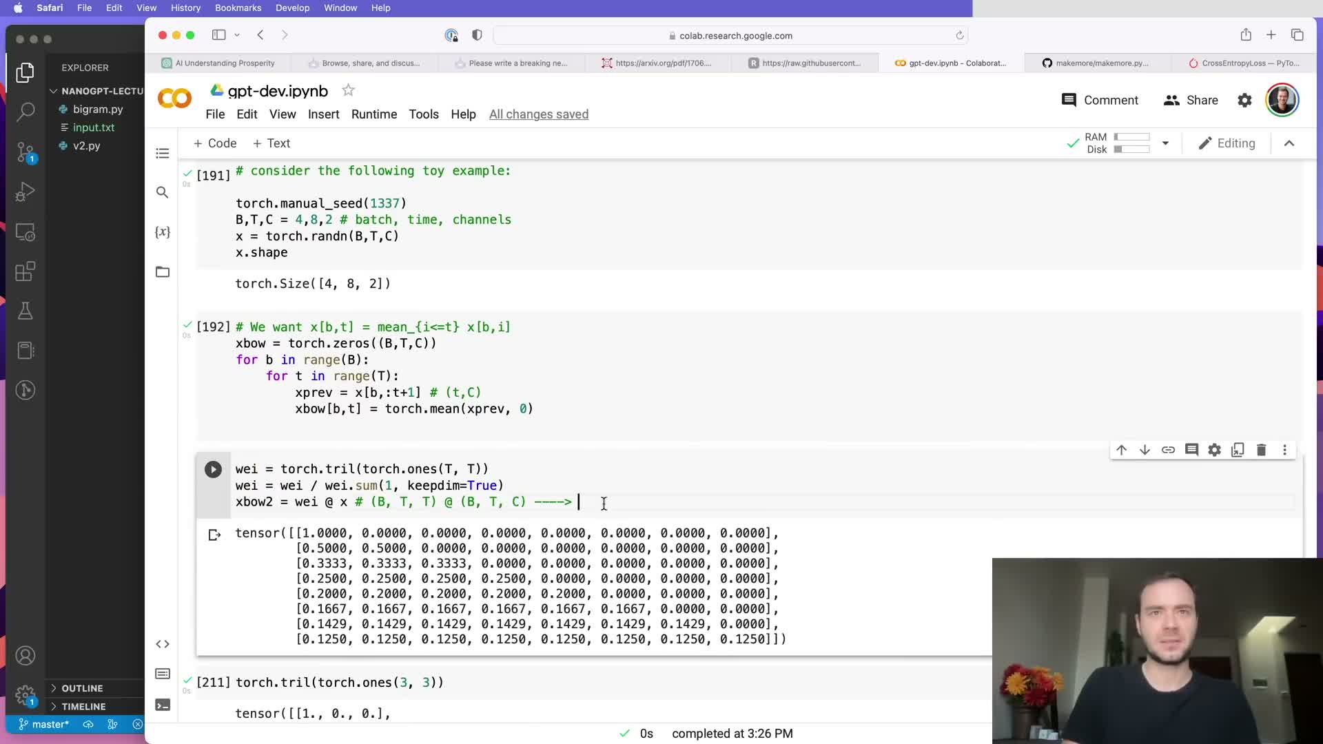
Lower-triangular weight matrices and batched matrix multiplication vectorize prefix aggregation.
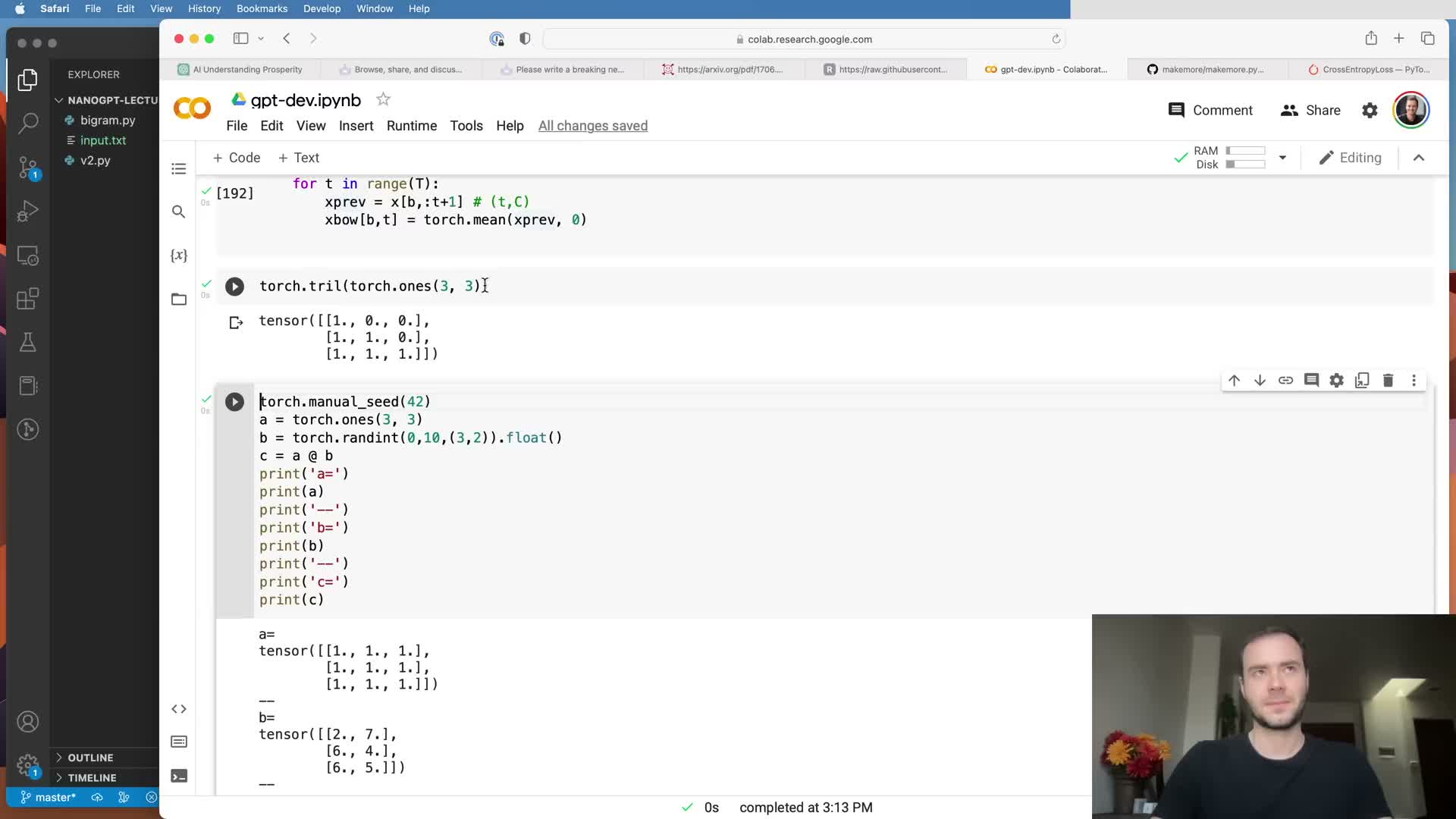
A lower-triangular binary matrix of ones can sum all prefixes for each position via a single batched matrix multiplication:
- Multiply a (T, T) lower-triangular matrix by a (B, T, C) token tensor to produce (B, T, C) prefix sums.
- Normalizing the rows of the triangular matrix yields prefix averages instead of sums.
- Using batched GEMM applies this operation independently across batch elements and eliminates explicit loops, yielding large performance gains on GPUs.
This matrix formulation is the algebraic foundation enabling efficient masked attention implementations.
Masking with negative infinity and softmax produces normalized, causal affinity weights.
To enforce causality in attention, set the non-allowed (future) entries of the T×T weight matrix to negative infinity and then apply softmax across each row:
- Filling masked positions with -inf ensures their contribution becomes zero after exponentiation and normalization, enforcing autoregressive constraints.
- Parameterize the unmasked entries as learnable affinities so the model can compute data-dependent weights via softmax to selectively aggregate information.
This masked softmax pattern is the computational primitive that enables causal attention in decoders.
Introduce embeddings and an output projection to separate token identity and model dimensionality.
Replace the trivial logits-as-embeddings approach with:
- A token embedding of dimension embed_dim.
- A separate linear language modeling head that projects model features back to vocabulary logits.
Also:
- Add positional embeddings indexed by time position and add them to token embeddings so attention can distinguish positions.
- Combined token + positional embeddings form the input representations consumed by subsequent attention layers.
This decouples embedding dimensionality from vocabulary size and enables richer continuous feature spaces.
Self-attention computes data-dependent affinities via query-key dot products and aggregates values accordingly.
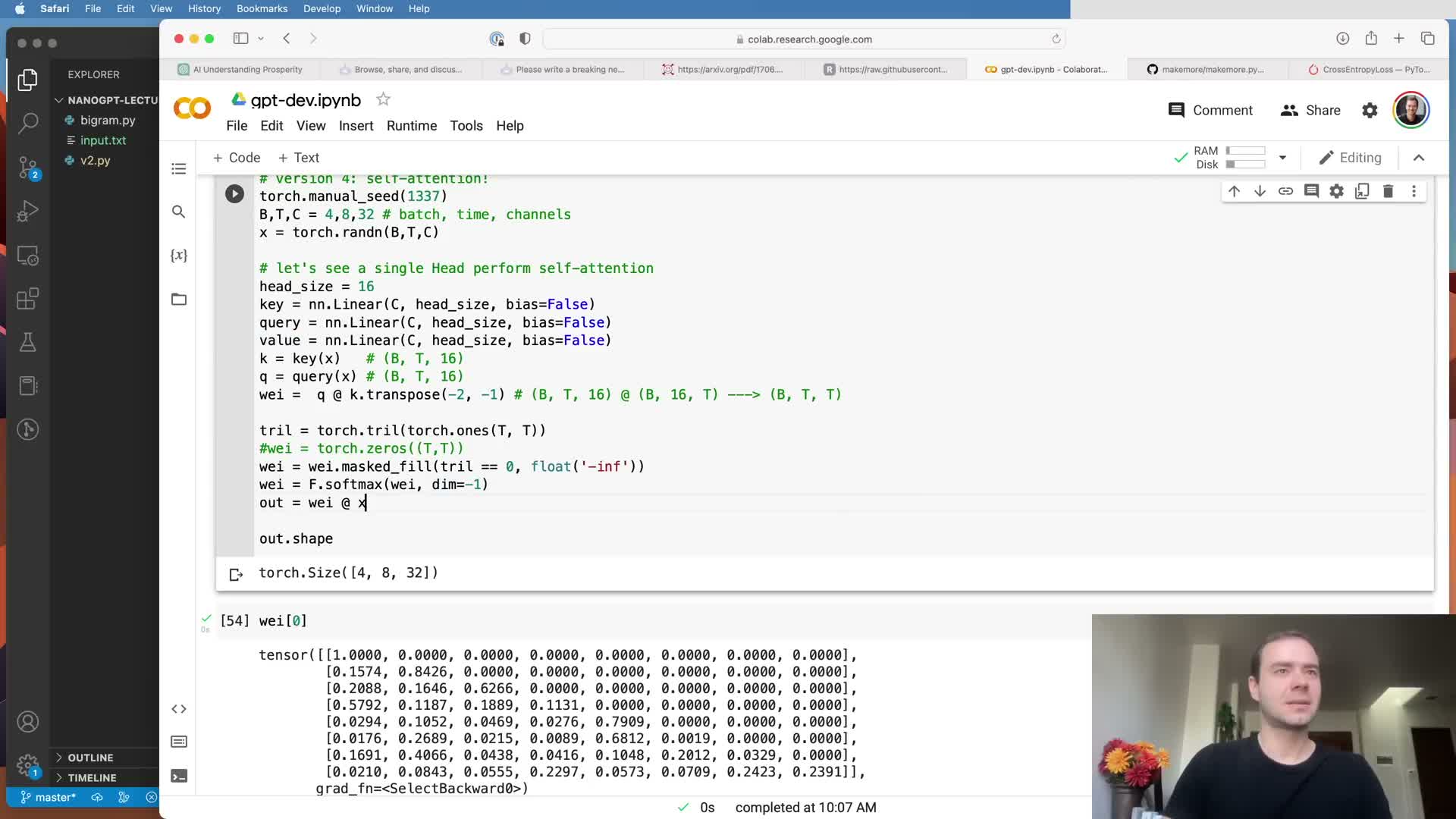
Each token emits three learned linear projections: query (Q), key (K), and value (V) vectors.
Computation steps:
- Compute affinities as Q × Kᵀ (batched) to obtain a B × T × T affinity tensor.
- Apply causal masking and softmax to convert affinities into normalized attention weights.
- Multiply these weights with the V matrix to produce aggregated, context-aware outputs per position.
The output dimension equals the head size and captures information from selected past tokens weighted by their learned relevance.
Attention is a general communication mechanism with graph and positional considerations.
Interpretation and generalization of attention:
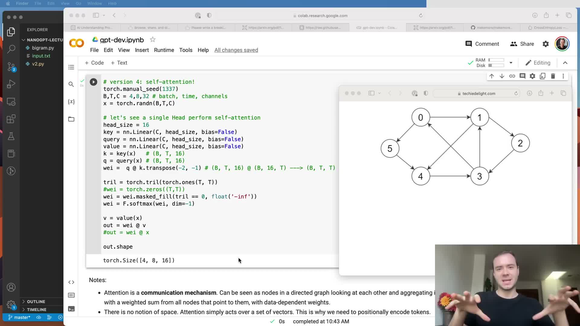
- Attention is directed communication in a graph where nodes aggregate weighted information from neighbors; in autoregressive modeling the connectivity is triangular to prevent future→past flow.
- Attention operates on unordered sets of vectors, so positional encodings are required to inject sequence order.
- Batch elements are independent pools of nodes processed in parallel with batched matrix ops.
- Attention generalizes to encoder-decoder and cross-attention when queries and keys/values originate from different sources; mask and connectivity choices tailor attention to the task.
Scale dot-product attention by 1/sqrt(d_k) to control variance and softmax sharpness.
When Q and K vectors have approximately unit variance, their dot product variance grows with head dimensionality; divide dot products by sqrt(d_k) to stabilize the attention logits.
Rationale:
- Scaling prevents the softmax from becoming extremely peaky at initialization and preserves diffuse weight distributions that allow gradients to propagate.
- Without scaling, larger head sizes would produce overly confident one-hot attention distributions and hamper learning, especially early in training.
This scaled dot-product formulation is standard practice in Transformer implementations.
Implement a single self-attention head module and integrate it into the model while enforcing context cropping.

Encapsulate key-query-value projections, the causal triangular mask (as a non-parameter buffer), scaled dot-product computation, softmax normalization, and value aggregation into a reusable Head class.
Implementation tips:
- Register the lower-triangular mask as a buffer so it moves with the module across devices but is not treated as an optimizer parameter.
- During autoregressive generation, crop the input context to at most block_size to match positional embedding capacity and avoid index overflow.
This modular head becomes the building block for multi-head attention and deeper stacks.
Training with a single scaled attention head yields modest gains, while multi-head attention improves representation capacity.
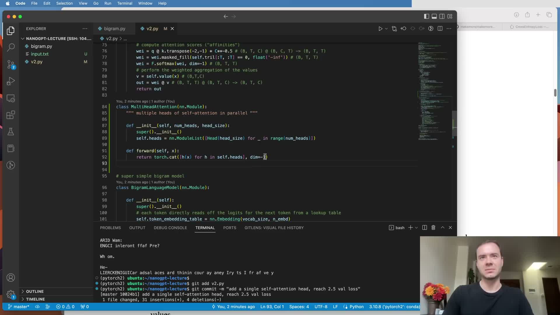
Replacing the bigram model with a single self-attention head enables data-dependent communication across positions and typically reduces validation loss modestly.
Extending to multi-head attention:
- Creates parallel communication channels (heads) that each capture different pairwise or feature-specific interactions.
- Concatenate head outputs and project back to the embedding dimension to enrich representational capacity.
- Empirically, multi-head attention reduces validation loss further vs. a single head and is analogous to grouped convolutions where separate groups learn complementary patterns.
Add a per-position feed-forward network to allow tokens to process gathered context independently.

After attention aggregates information across positions, apply a position-wise MLP (linear → nonlinearity → linear) independently to each token to let it transform and reason about the aggregated context.
Notes:
- The feed-forward block is applied identically and independently at each time position, complementing communication from attention.
- Interleaving attention and feed-forward layers allows the model to both exchange information and elaborate features hierarchically.
- Adding this stage typically improves expressivity and validation performance.
Stack Transformer blocks with residual projections to enable deep architectures.

Compose Transformer blocks that intersperse multi-head self-attention and position-wise feed-forward layers, include residual (skip) connections around each sub-layer, and project back to the embedding dimension.
Why this structure matters:
- Residual connections provide gradient highways that preserve signal from later loss gradients back to earlier layers, making deep networks feasible and improving optimization dynamics.
- Apply a linear projection after concatenated multi-head outputs to return to the residual pathway and enable parameter-efficient composition.
- This block structure is the canonical Transformer decoder block used in GPT-style models.
Use feed-forward inner expansion and LayerNorm (pre-norm) to stabilize training.
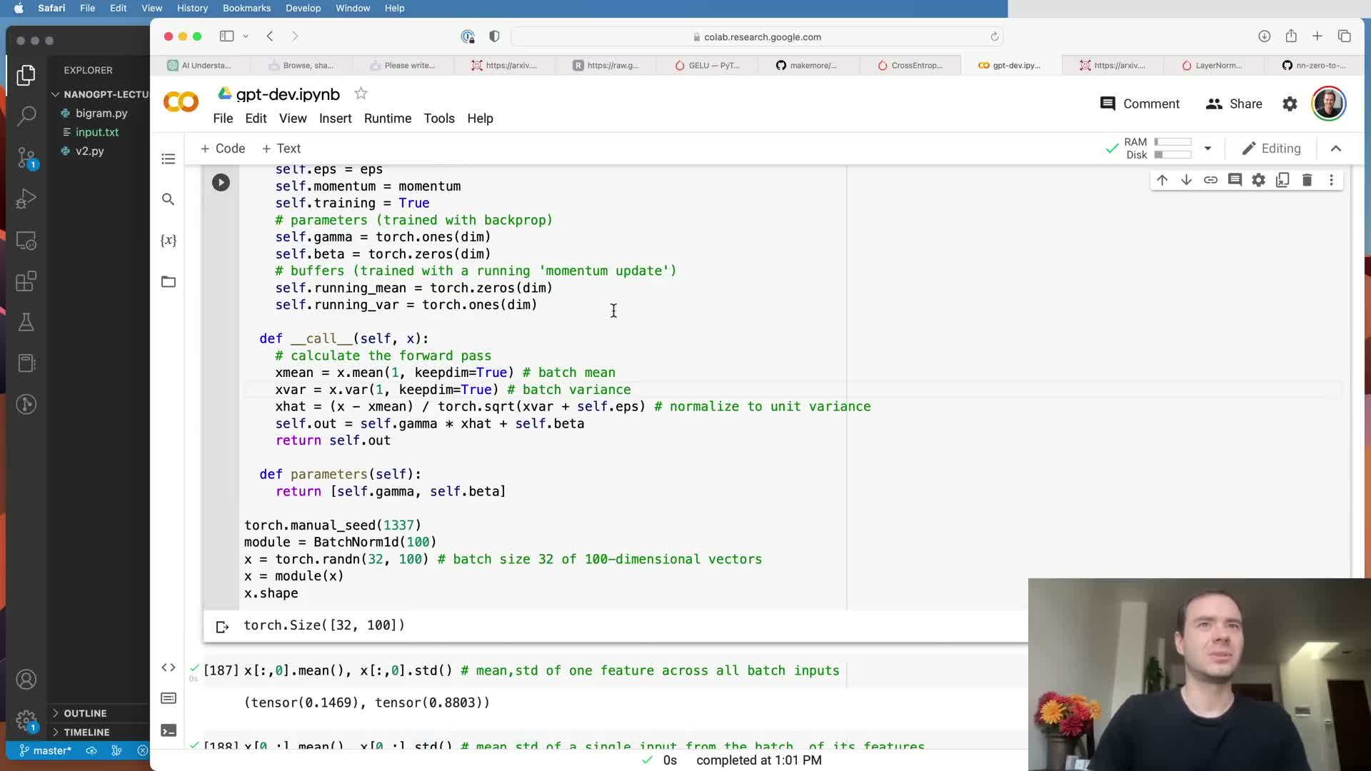
Expand the feed-forward inner layer dimensionality (commonly a factor of four) to increase per-token computation capacity, and apply LayerNorm before each sub-layer (pre-norm) to normalize feature statistics at initialization.
Practical benefits:
- Pre-norm LayerNorm normalizes across the embedding dimension per token and includes learned scale and bias.
- These choices improve gradient conditioning compared to post-norm in many setups, reducing training instability in deeper stacks.
- Together with residuals and inner expansion, pre-norm LayerNorm fosters faster convergence and better final performance.
Add dropout and scale up model hyperparameters to improve generalization and capacity.
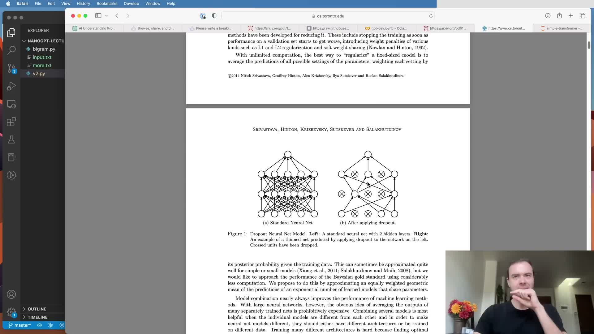
Introduce dropout on attention probabilities and residual outputs as regularization that randomly zeroes activations during training.
Scaling model capacity:
- Increase batch size, block size (e.g., 256), embedding dimension (e.g., 384), number of heads, number of layers, and adjust learning rate appropriately.
- With moderate scaling and GPU training (e.g., A100), validation loss can drop substantially, showing how capacity and regularization jointly drive gains.
- Larger models require careful regularization and hyperparameter tuning to remain optimizable.
A decoder-only Transformer implements autoregressive language modeling; encoder-decoder variants support conditioned sequence-to-sequence tasks.
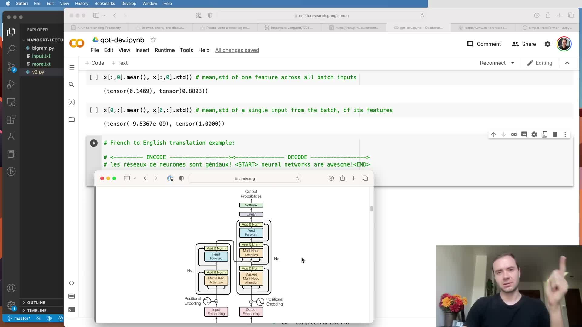
The implemented model is a decoder-only Transformer that uses causal masking so tokens cannot attend to future positions, making it suitable for unconditioned autoregressive generation (as in GPT).
Contrast with the original architecture:
- “Attention Is All You Need” used an encoder-decoder configuration for sequence-to-sequence tasks (e.g., translation): the encoder processes source tokens with full bidirectional attention and the decoder cross-attends to encoder outputs.
-
Decoder-only models omit the encoder and cross-attention, simplifying the architecture for pure language modeling.
- To turn a pre-trained decoder into an assistant-like agent (e.g., ChatGPT), additional fine-tuning and alignment stages are required.
Large-scale models require pre-training on massive corpora then fine-tuning and alignment to become useful assistants.
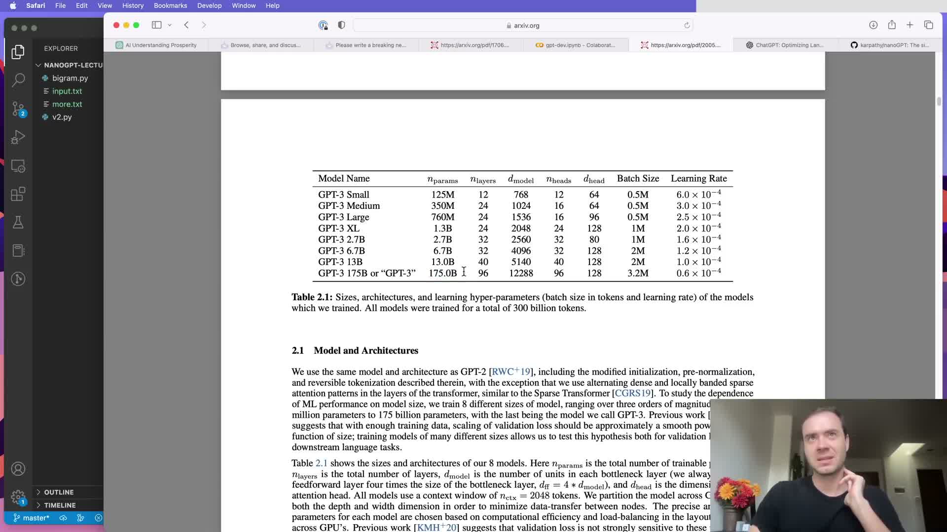
Pre-training and alignment pipeline overview:
-
Pre-training: train a large decoder-only Transformer on vast corpora of internet text to learn general language modeling capabilities — model and token scale during pre-training determine much downstream capability.
-
Supervised fine-tuning: adapt the generic model on labeled question-answer pairs and other supervised datasets.
-
Preference learning: collect human preference data and train a reward model to score outputs.
-
Reinforcement Learning from Human Feedback (RLHF): optimize the sampling policy (e.g., via PPO) against the reward model to produce controlled, helpful, and safe assistant behavior.
These alignment stages are often data- and compute-intensive beyond pre-training.
NanoGPT implementation details and summary of the educational reproduction.
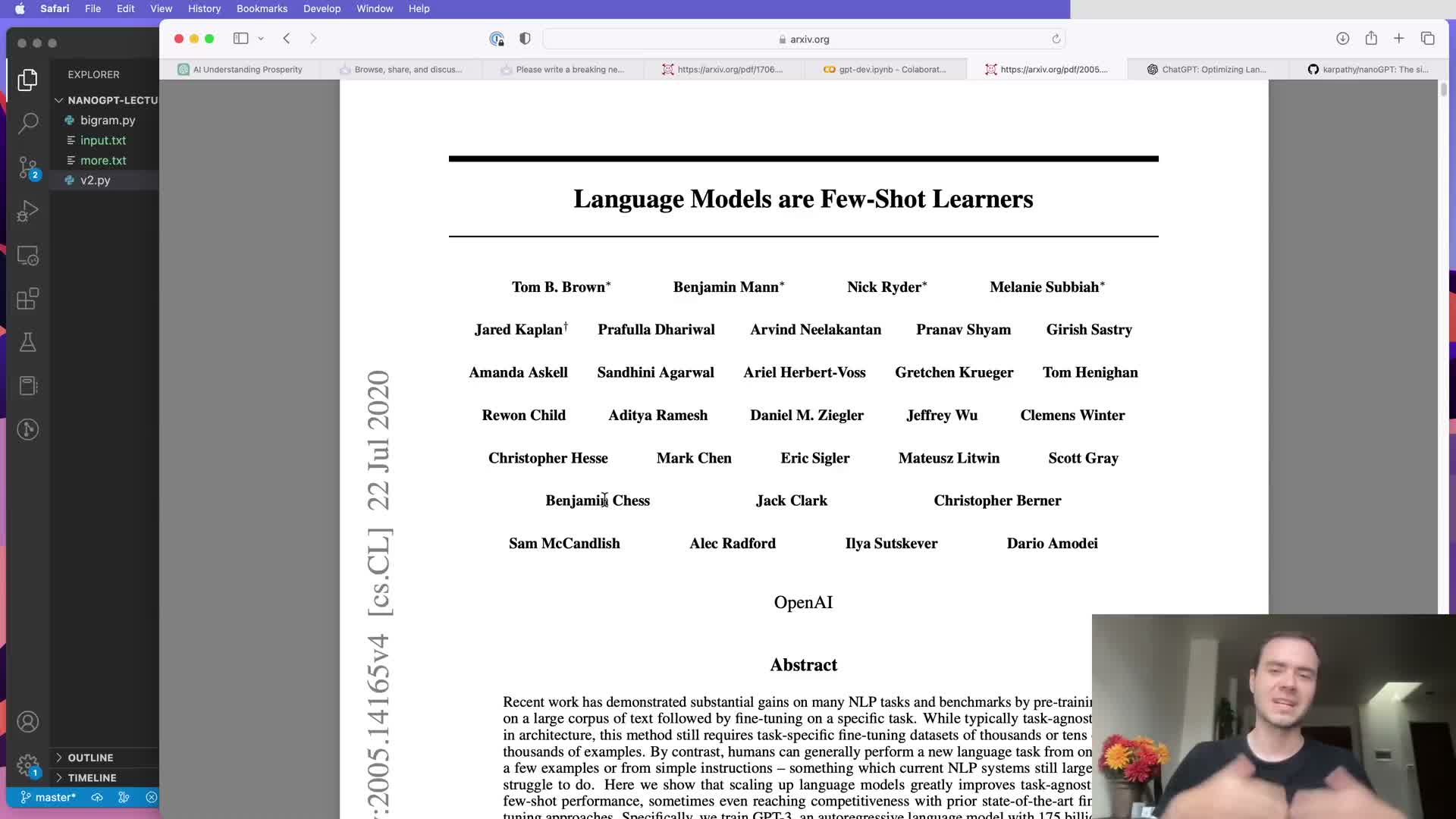
NanoGPT separates model definition and training utilities into concise files (e.g., model.py and train.py) and implements core Transformer features consistent with standard GPT variants.
Included practicalities:
- Causal self-attention, multi-head aggregation, position-wise MLPs, LayerNorm, residual projections, and generation routines.
- Checkpointing, selective weight decay, optional dropout, device management, and support for scaling/loading checkpoints.
- Educational reproduction shows a complete Transformer-based language model can be implemented in a few hundred lines and, when scaled appropriately on GPU, produce plausible Shakespeare-like output from a small corpus.
The project focuses on the pre-training stage and leaves complex alignment pipelines (reward models, RLHF) as higher-level extensions.
Enjoy Reading This Article?
Here are some more articles you might like to read next: