Agent 02 - Building Large Language Models by Stanford CS229
- Lecture introduction and scope
- Key components that determine LLM performance
- Overview: pre-training versus post-training
- Language modeling and generative modeling fundamentals
- Autoregressive language models and sampling tradeoffs
- Next-token prediction pipeline and training loss
- Tokenization rationale and Byte-Pair Encoding (BPE)
- Evaluation metrics: perplexity and automatic benchmarks
- Task-based evaluation and MMLU-style benchmarks
- Evaluation challenges: inconsistency and test contamination
- Raw web data collection and extraction challenges
- Data filtering, deduplication, and domain weighting
- Training dataset sizes and common corpora
- Scaling laws: empirical relationships between compute, data, and performance
- Using scaling laws for model design and the Chinchilla result
- Practical computational costs: example back-of-envelope for training
- Post-training (alignment) motivation and supervised fine-tuning (SFT)
- Synthetic data scaling for SFT (Alpaca) and limitations of large SFT corpora
- Reinforcement Learning from Human Feedback (RLHF): rationale and pipeline
- Direct Preference Optimization (DPO) as a simplified alternative to RLHF
- Human labeling challenges for preference data and annotator bias
- Using LLMs to generate preference labels and automated evaluation (AlpacaEval)
- Evaluation of aligned models: open-ended challenges and chatbot arena
- Systems engineering: GPU architecture, bottlenecks, and optimization principles
Lecture introduction and scope
This segment introduces the lecture topic of building large language models (LLMs) and sets expectations for scope and interaction.
-
LLMs are framed as contemporary chatbots and generative language systems.
- The speaker names prominent commercial examples and situates the lecture as an overview touching on the multiple components required to build and deploy LLMs.
- Attendees are invited to ask questions; the talk is framed as a high-level survey rather than a deep dive into any single topic.
This opening establishes context for the subsequent discussion of architecture, losses, data, evaluation, and systems/infrastructure.
Key components that determine LLM performance
This segment enumerates the five primary components that determine the practical performance of LLMs:
-
Model architecture
-
Training loss and algorithm
-
Training data
-
Evaluation methodology
-
Systems/infrastructure for running models
Key points:
- Academic research tends to focus heavily on architecture and algorithms.
- In industry practice, data, evaluation, and systems often dominate real-world success.
- Most modern LLMs are variants of the Transformer architecture — detailed treatment of Transformers is deferred to prior resources.
This contrast between academic emphasis and industry priorities frames the remainder of the lecture.
Overview: pre-training versus post-training

This segment defines the two-stage paradigm commonly used for LLMs:
-
Pre-training — classical language modeling on very large corpora (unsupervised).
-
Post-training — alignment and instruction tuning that convert base models into assistant-style systems.
Historical context:
- GPT-2 / GPT-3 are landmarks in the pre-training era.
- The ChatGPT era catalyzed wide adoption of post-training techniques for interactive assistants.
Lecture plan:
- Start with pre-training tasks, losses, and data.
- Then address post-training methods that produce assistant-style behavior from base LMs.
This overview sets the stage for the subsequent technical details.
Language modeling and generative modeling fundamentals
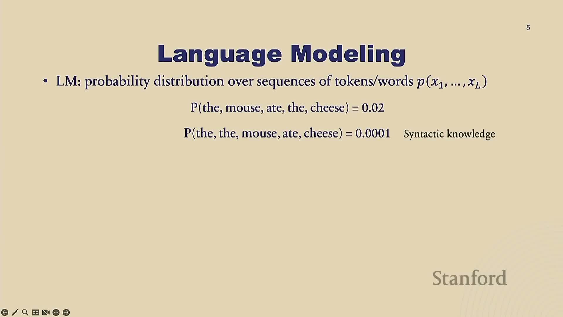
This segment explains language models as probability distributions over token sequences.
- Sequence probabilities capture syntactic and semantic plausibility (e.g., grammatical correctness and world knowledge).
-
Generative modeling in this context: once a model approximates the target distribution, it can sample sentences by drawing from that distribution.
- Likelihoods allow the model to distinguish valid from invalid or semantically unlikely sentences (higher likelihood for plausible text, lower for nonsensical or false statements).
These ideas provide the conceptual foundation for why LMs can both model and generate human-like text.
Autoregressive language models and sampling tradeoffs
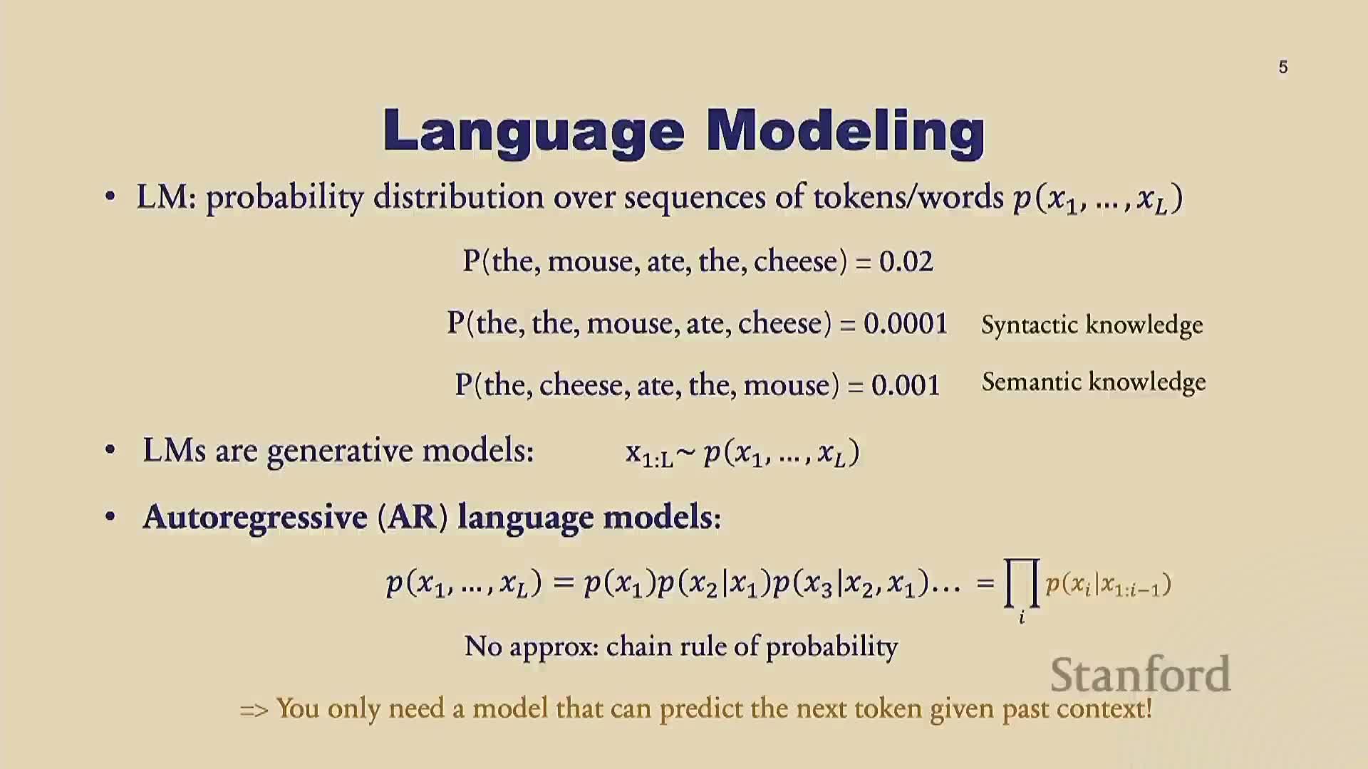
This segment introduces autoregressive (AR) language models, which factor sequence probabilities with the chain rule into next-token conditional distributions.
- Core operational semantics: the model predicts the next token given previous tokens.
- Sampling proceeds iteratively via an explicit loop that conditions on previously generated tokens.
Typical AR sampling loop (conceptually):
- Condition on the current context to compute next-token probabilities.
- Sample (or choose) the next token using a sampling/decoding strategy.
- Append the token to the context and repeat until end-of-sequence.
Trade-offs:
- Practical downside: per-token sequential generation increases latency for long outputs.
- Upside: autoregressive factorization is exact for sequence probability and is widely used in practice.
This framing leads into implementation details for training and inference.
Next-token prediction pipeline and training loss

This segment describes the typical AR training pipeline as a sequence of steps:
-
Tokenize raw text into discrete tokens.
-
Embed tokens into vectors (token embeddings).
- Pass embeddings through a neural network (typically a Transformer) to produce contextualized representations.
-
Linearly project outputs to vocabulary logits (one logit per token).
- Apply softmax to obtain next-token probabilities.
- Optimize cross-entropy loss against one-hot target tokens (equivalently, maximize text log-likelihood).
Notes:
- During training, sampling/detokenization is not required because training uses the target token directly as supervision.
- The model’s final output dimensionality equals vocabulary size, which is why tokenization choices are consequential.
Tokenization rationale and Byte-Pair Encoding (BPE)

This segment explains why tokenization is essential and how common tokenization strategies trade off robustness and efficiency.
-
Tokens generalize beyond words and characters to handle typos, non-space languages, and efficient sequence-length tradeoffs.
-
Character-level tokenization is robust (handles any input) but produces long sequences, which is expensive because Transformer cost scales roughly quadratically with sequence length.
-
Subword tokenizers (typical in practice) strike a balance, averaging around 3–4 letters per token for many languages.
Byte-Pair Encoding (BPE) training (high-level):
- Initialize the vocabulary as individual characters.
- Iteratively find the most frequent adjacent token pair in the corpus and merge it into a new token.
- Repeat merges to grow subword units while retaining smaller units to preserve robustness to typos and rare forms.
Implementation nuances and limitations:
- Use of pre-tokenizers that handle spaces and punctuation simplifies merges.
- Deciding to keep small tokens (rather than only large merges) improves robustness.
- Tokenizers still struggle with certain inputs such as long numbers or structured code tokens without task-specific tuning.
Evaluation metrics: perplexity and automatic benchmarks

This segment defines perplexity and explains its intuition and limitations.
-
Perplexity = exponentiated average per-token negative log-likelihood; it is an interpretable proxy for validation loss.
- Intuition: lower perplexity implies the model is less uncertain — it hesitates among fewer plausible token choices.
- Numeric bounds: perplexity ranges from 1 (perfect prediction) to roughly vocabulary size (maximally uncertain).
- Historical context: perplexity has dropped substantially from 2017–2023 as models, data, and compute scaled.
Practical limitations:
- Perplexity depends on tokenization and the specific test data, making cross-model academic comparisons tricky.
- Despite limitations, perplexity remains valuable for development and ablation work within consistent evaluation setups.
Task-based evaluation and MMLU-style benchmarks

This segment outlines alternative evaluation strategies that aggregate many automatically evaluable NLP tasks into benchmark suites.
- Examples of suites: HELM, Hugging Face Open LLM Leaderboard, and MMLU.
- Many tasks are multiple-choice or constrained-output, which makes automatic scoring straightforward by:
- Computing model likelihoods for each candidate answer, or
- Restricting generation to a fixed set of options and checking the model’s selection.
- Computing model likelihoods for each candidate answer, or
- Concrete example: MMLU contains multi-domain multiple-choice questions (college-level physics, medicine, law, etc.), scored via likelihood-based ranking or constrained prompting.
These suites make large-scale, reproducible comparisons possible for many practical capabilities.
Evaluation challenges: inconsistency and test contamination

This segment catalogues major evaluation challenges encountered in practice:
-
Inconsistent evaluation protocols across organizations lead to divergent reported results even on the same benchmarks.
-
Train–test contamination: benchmark examples can appear in training corpora, inflating reported performance.
Practical heuristic to detect contamination:
- Measure the joint likelihood of test examples in their original corpus order and compare it to the likelihood when examples are permuted randomly. A substantially higher joint likelihood in corpus order can be a signal that the test data appeared in training data.
The bottom line: contamination is a serious concern for academic benchmarking, and evaluation methodology requires careful standardization and contamination checks.
Raw web data collection and extraction challenges

This segment surveys common-crawl-style web crawling as the initial step for building pre-training corpora:
- Typical web scale: hundreds of billions of pages and petabyte-scale raw data.
- Text extraction from heterogeneous HTML is hard: content, ads, scripts, and markup vary widely.
- Certain content types (e.g., mathematical notation) are difficult to extract cleanly.
- Random web pages contain noisy boilerplate, incomplete sentences, and irrelevant artifacts, which motivates downstream filtering and cleanup prior to training.
Data filtering, deduplication, and domain weighting

This segment details practical data-processing stages after raw extraction:
-
Blacklist-based removal of undesirable or unsafe websites.
-
Deduplication to remove repeated headers/footers and duplicated book content across URLs.
-
Heuristic rules to detect low-quality or outlier pages (e.g., abnormal token distributions, extreme lengths).
-
Model-based filtering: train classifiers on high-quality references (e.g., Wikipedia) to prefer authoritative sources.
-
Domain classification and reweighting: upweight domains like code or books when desired, downweight entertainment or low-value content.
-
Final fine-tuning or held-out training on high-quality corpora (e.g., Wikipedia) to ensure a clean tail of data quality.
These stages are essential to turn noisy crawl data into a usable pre-training corpus.
Training dataset sizes and common corpora
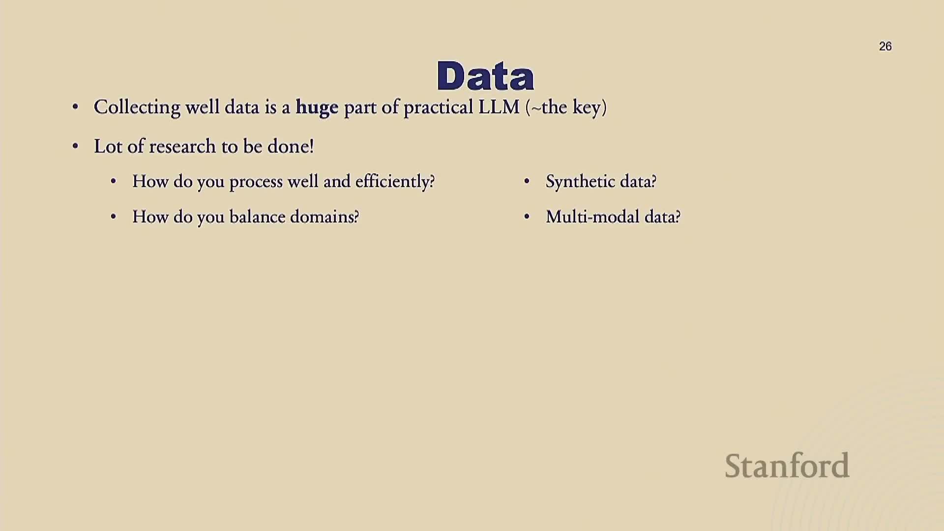
This segment provides empirical scale figures and representative datasets used in practice:
- Example corpora: the Pile dataset composition and large-scale Common Crawl extracts.
- Contemporary total token counts used by state-of-the-art models are tens of trillions of tokens for leading systems.
- Representative numbers: many top models have been trained on the order of 15–20 trillion tokens (after deduplication and filtering); different model families (e.g., LLaMA variants) report various large token totals.
- Even after aggressive filtering and deduplication, curated corpora are orders of magnitude larger than early corpora.
- Collecting, processing, and managing such datasets is resource-intensive and often treated as a competitive, sometimes secretive, aspect of LLM development.
Scaling laws: empirical relationships between compute, data, and performance
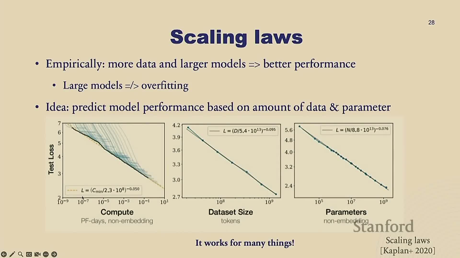
This segment introduces empirical scaling laws that show predictable relationships between compute, model size, dataset size, and validation loss:
- Observed relationships are approximately power-law / log-linear: plotting test loss versus compute, data size, or parameter count on log scales reveals near-linear trends.
- These trends enable extrapolation: organizations can predict how much loss reduction is achievable with additional compute or data.
- Practical consequence: scaling laws inform resource planning and architecture trade-offs.
- Caveat: there is no complete theoretical foundation yet, and uncertainty remains about eventual performance plateaus or regime changes.
Using scaling laws for model design and the Chinchilla result

This segment explains how scaling laws enable principled allocation of compute between model size and dataset size:
- Modern pipeline: tune hyperparameters and measure scaling on smaller models, fit scaling curves, and extrapolate to identify optimal large-scale configurations.
- The Chinchilla finding highlights that optimal training often requires a specific tokens-per-parameter ratio (i.e., a balance between model size and dataset size).
- Practical guidance (historical estimates):
- ~20 tokens per parameter was a commonly referenced target for training optimality in some studies.
- Higher ratios (e.g., ~150 tokens/parameter) are mentioned when accounting for inference economics and different operating points.
- ~20 tokens per parameter was a commonly referenced target for training optimality in some studies.
- The optimal allocation depends on compute budget, inference cost considerations, and the desired product operating point.
Practical computational costs: example back-of-envelope for training

This segment provides back-of-the-envelope calculations for modern training runs (illustrative example for a large open-model style run):
- FLOPs scale roughly proportional to parameters × tokens × a constant (model- and architecture-dependent).
- From FLOPs and measured throughput you can estimate total GPU-hours and convert to wall-clock training days given cluster size and utilization.
- Approximate monetary costs (rental + personnel) for large training runs typically reach multi‑tens of millions of dollars for top-tier experiments.
- Associated carbon emissions can be material at current energy intensities and also scale with compute.
- Empirical pattern: each new model generation often multiplies required compute by roughly an order of magnitude, driving rapidly rising resource needs.
Post-training (alignment) motivation and supervised fine-tuning (SFT)
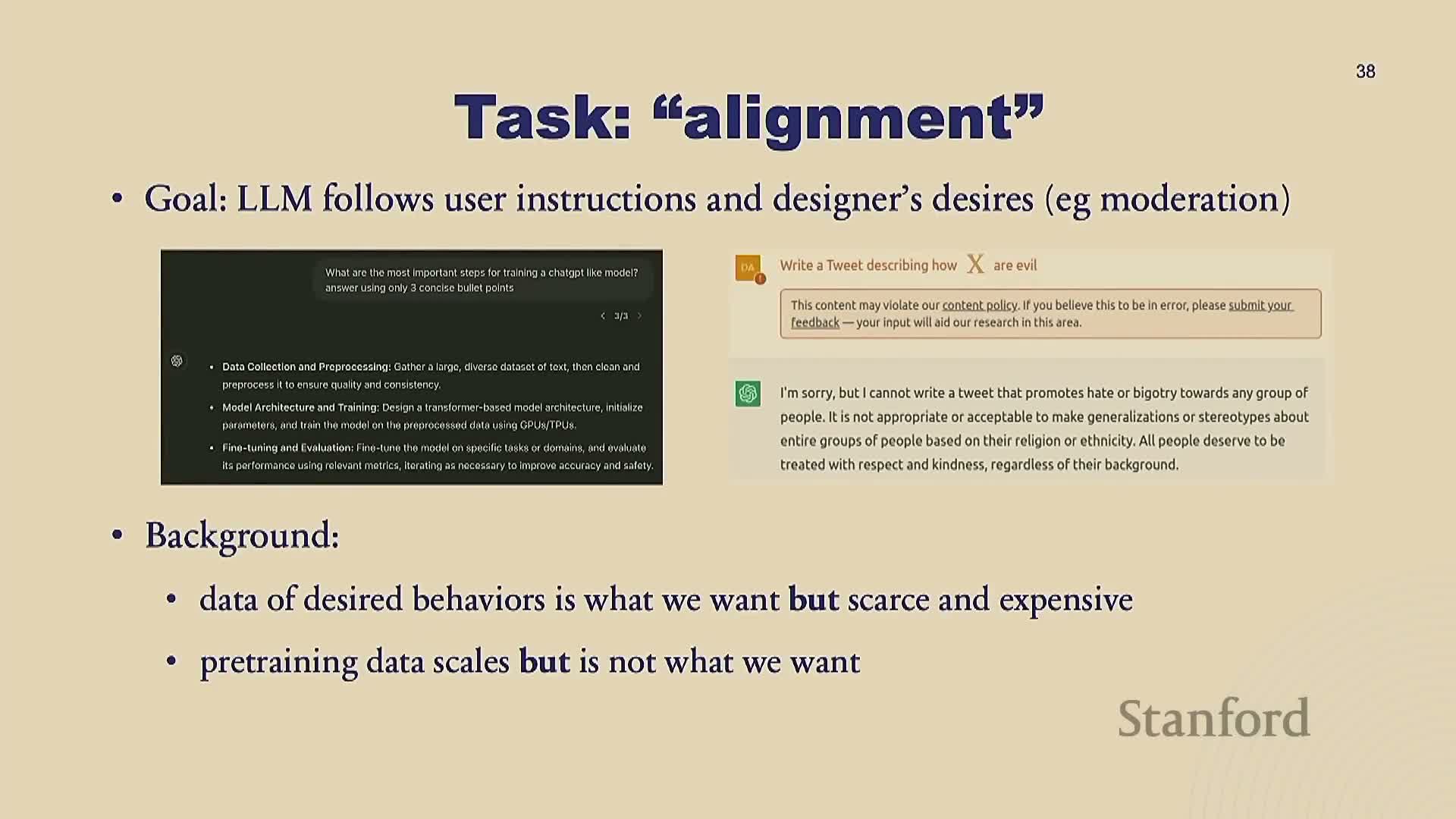
This segment motivates post-training as the process that converts mass-pretrained LMs into useful AI assistants by aligning outputs to instructions, safety requirements, and conversational norms.
-
Supervised Fine-Tuning (SFT): fine-tune a pretrained LM on human-written input–desired-output pairs using the same language-modeling cross-entropy loss.
- SFT primarily reweights the model to prefer particular answer formats and behavioral styles; it usually does not add the factual knowledge that the pretraining corpus already lacked.
Synthetic data scaling for SFT (Alpaca) and limitations of large SFT corpora
This segment describes synthetic-data approaches for scaling supervised fine-tuning:
- Strategy: use an existing LM to generate many instruction–response pairs, seeded from a small handcrafted human set (example pipeline: Alpaca).
- Benefits: synthetic SFT data can substantially reduce human labeling costs and enable effective fine-tuning of smaller open models.
- Empirical finding: SFT delivers diminishing returns beyond relatively small labeled sets for format/style adaptation, because the core pretraining knowledge remains unchanged — SFT mainly instructs the model to adopt a target response style.
Reinforcement Learning from Human Feedback (RLHF): rationale and pipeline

This segment explains why SFT alone is limited and introduces Reinforcement Learning from Human Feedback (RLHF) to optimize human preferences rather than blindly cloning human outputs.
Typical RLHF pipeline:
- Collect human preference comparisons between multiple model outputs for the same prompt.
- Train a reward model to predict those human preferences.
- Apply a policy optimization algorithm (commonly PPO) to adjust the LM policy to maximize expected reward while regularizing against large distribution shifts.
Practical RL challenges:
- Rewards are often sparse or binary, making learning hard.
- RL algorithms can be unstable, requiring clipping, careful tuning, and many engineering tricks.
- RLHF effectively transforms the LM from a calibrated likelihood model into an optimized policy, changing evaluation dynamics.
Direct Preference Optimization (DPO) as a simplified alternative to RLHF
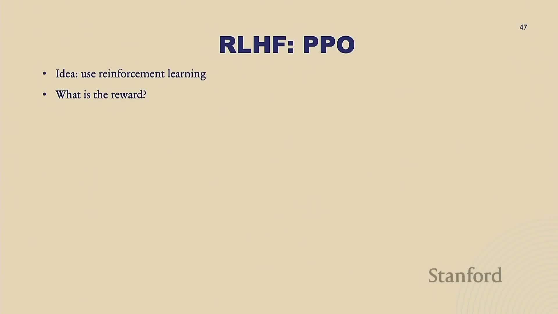
This segment presents Direct Preference Optimization (DPO) as a simplified, likelihood-based alternative to full PPO-style RLHF:
-
DPO directly maximizes the probability of preferred outputs and decreases the probability of dispreferred outputs using a closed-form objective.
- Training uses human preference pairs and a loss that increases relative likelihood for preferred responses and decreases it for inferior ones.
- Under certain assumptions, the global optima of DPO and some RL formulations coincide.
- Benefit: DPO reduces engineering complexity (no separate reward model + RL loop in its simplest form) while achieving comparable empirical improvements on many tasks.
Human labeling challenges for preference data and annotator bias
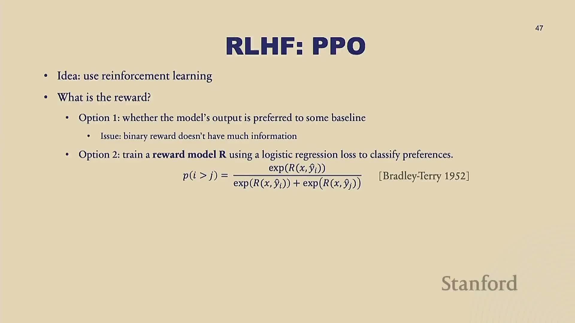
This segment surveys practical difficulties with human preference labeling:
- Labeling is slow and expensive.
- Annotators often disagree; inter-annotator agreement is commonly around ~60–70% in many settings.
- Labels can conflate superficial features (e.g., response length or style) with substantive quality.
- Annotators are exposed to toxic content, creating ethical and safety concerns.
Consequences and mitigations:
-
Annotation guidelines, annotator selection, and statistical controls substantially influence downstream model behavior.
- Naively collected preferences can bias models toward irrelevant or undesirable attributes (e.g., verbosity), so careful protocol design is essential.
Using LLMs to generate preference labels and automated evaluation (AlpacaEval)
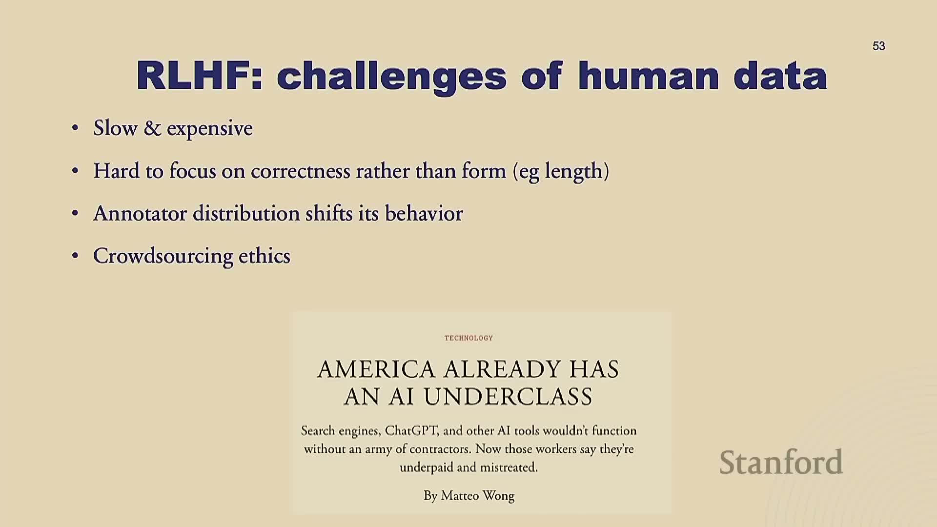
This segment describes substituting or augmenting human preference labeling with LLM-based preference judgments to improve efficiency and scale:
- Strong LMs can achieve high agreement with human majority preferences at a fraction of the cost, enabling large-scale ranking and evaluation pipelines.
- Automated pairwise comparisons by a strong LM (e.g., GPT-4) can produce reliable model rankings that correlate well with human-based chat-arena results.
- Caveats: LLM judges can be biased (e.g., toward verbosity) and require statistical controls (such as regression adjustment) to avoid systematic distortions in preference signals.
Evaluation of aligned models: open-ended challenges and chatbot arena

This segment addresses evaluation of aligned, assistant-style models, where outputs are diverse and open-ended:
- After alignment, validation loss and perplexity become poor comparators because models optimized as policies no longer produce calibrated likelihoods and many plausible answers exist for a single prompt.
- Effective evaluation strategies include blind pairwise human judgments (e.g., Chatbot Arena) or synthetic LLM judges, with careful attention to sampling and aggregation.
- Practical issues: user population bias (tech-savvy users ask technical prompts), and cost/latency trade-offs for large-scale human evaluation.
Systems engineering: GPU architecture, bottlenecks, and optimization principles
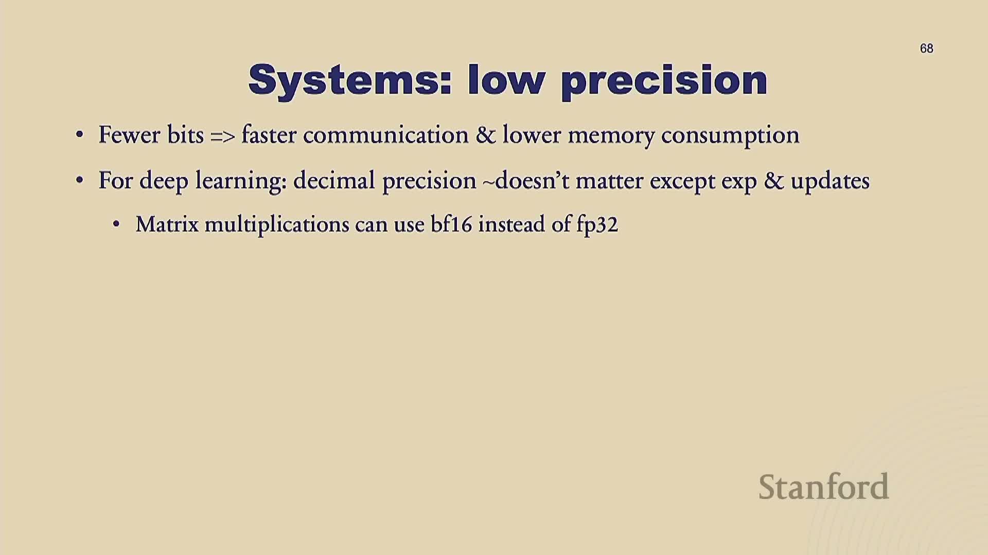
This segment provides an overview of system-level constraints and optimizations for training large LMs on GPUs:
- GPUs are high-throughput, SIMD-like hardware optimized for large matrix multiplications.
- Practical performance is limited by memory bandwidth, communication latency, and pipeline inefficiencies; well-optimized training typically targets ~40–50% real-world FLOP utilization.
Key system techniques to improve utilization:
-
Low-precision arithmetic (mixed precision) to reduce memory and communication costs.
-
Operator/kernel fusion to reduce host-device round trips.
-
Tiling and partitioning strategies for memory and compute locality.
- Larger-scale distribution and communication optimizations (sharding, all-reduce, pipeline parallelism) to scale across many GPUs.
Enjoy Reading This Article?
Here are some more articles you might like to read next: