MIT 6.S184 - Lecture 1 - Generative AI with SDEs
- Course introduction and learning objectives
- Representation of generative objects and formalizing generation via probability
- Conditional versus unconditional generation and conditional data distribution
- Generative model concept and the role of an initial distribution P_init
- High-level architecture: flow component versus diffusion component
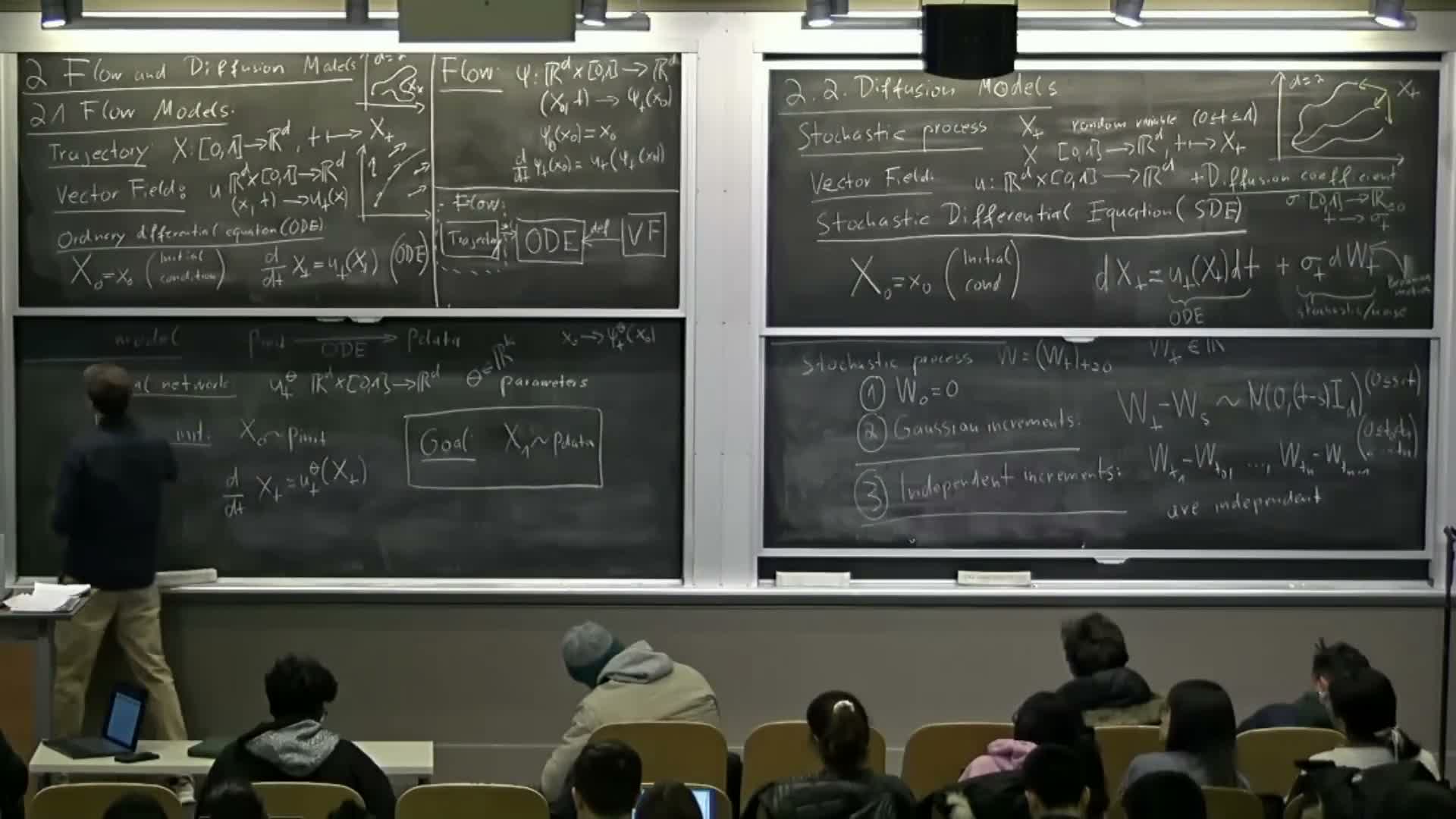
- Trajectory, vector field, and ordinary differential equation (ODE) definitions
- Flow map as a collection of ODE solutions and existence/uniqueness conditions
- Linear vector field example and analytic solution; numerical simulation by Euler method
- Flow models in machine learning: parameterizing the vector field with neural networks
- Sampling from a flow model and the practical sampling algorithm
- Motivation for diffusion models and introduction to stochastic differential equations (SDEs)
- Brownian motion: definition, Gaussian increments and independent increments
- Symbolic SDE notation and discretized increment interpretation
- Existence and uniqueness for SDEs and Euler–Maruyama simulation method
- Ornstein–Uhlenbeck linear SDE example and transition to diffusion model definition
- Sampling from diffusion models and practical considerations
- Course logistics, evaluation and resources
Course introduction and learning objectives
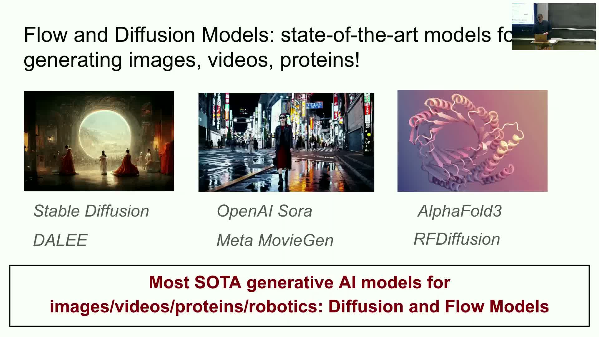
The course presents an intensive introduction to flow and diffusion generative models with emphasis on both theoretical foundations (ordinary and stochastic differential equations) and practical implementation through labs.
The material is framed around three primary goals:
-
Derive models from first principles — build models starting from fundamental continuous-time dynamics and probabilistic reasoning.
-
Teach the minimal required mathematics — cover only the mathematical tools needed to understand and work with flows and SDEs (ODEs, SDEs, vector fields, numerical integrators).
-
Provide hands-on implementation experience — labs that let students implement and experiment with image, video, and molecular generators so they can build end-to-end systems.
These goals are pursued in parallel: lectures for foundations, labs for implementation, and readings/examples to connect theory to practice.
Representation of generative objects and formalizing generation via probability
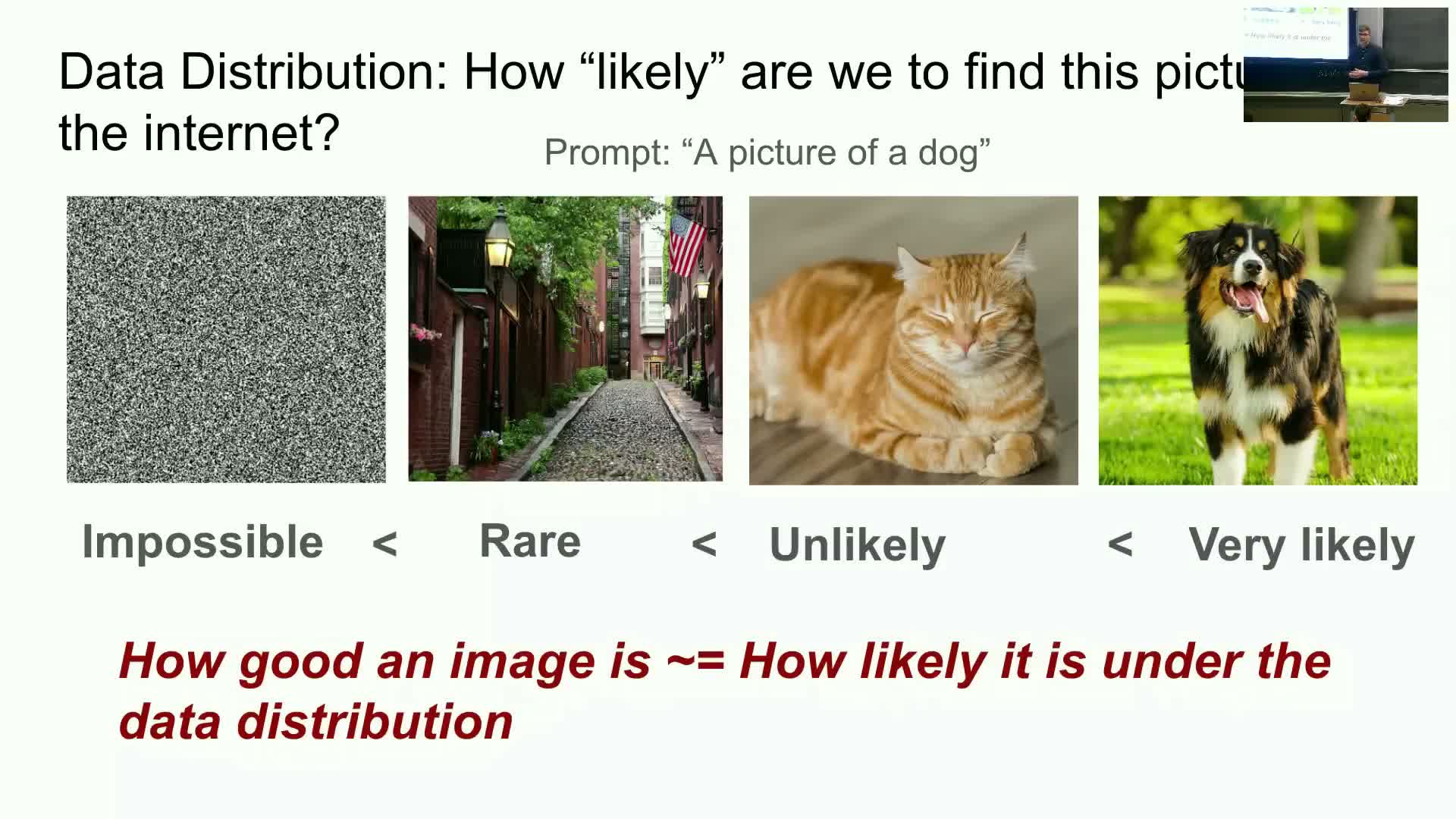
Digital objects to be generated (images, videos, molecular structures, etc.) are represented as vectors in R^d.
Generation is formalized as sampling from an unknown data distribution P_data defined over that vector space.
This formalization converts qualitative judgments of sample quality into a quantitative criterion: likelihood under P_data.
Consequently the learning objective becomes: produce a model whose samples are (approximately) drawn from P_data, turning generation into a statistical matching problem.
Conditional versus unconditional generation and conditional data distribution
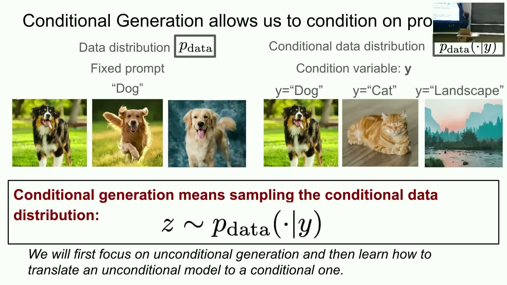
Unconditional generation produces samples from a single target distribution (for example, the distribution of all dog images).
| Conditional generation defines a conditional data distribution **P_data(x | y)** that specifies the distribution of objects x given a conditioning variable y (prompts, labels, text, or structured specifications). |
| Sampling conditionally means drawing x ~ **P_data(· | y), which enables **controllable generation. |
Conditional generation is the primary focus for subsequent modeling and training because it supports targeted, controllable outputs given y.
Generative model concept and the role of an initial distribution P_init
A generative model is an algorithm that transforms a simple, known initial distribution P_init (commonly an isotropic Gaussian) into the target data distribution P_data via a parameterized mapping.
The modeling goal is therefore to design a transform such that samples drawn from P_init and pushed through the model produce outputs whose distribution matches P_data.
In practice this means parameterizing a continuous-time or discrete mapping and optimizing its parameters so the terminal distribution aligns with the empirical data distribution.
High-level architecture: flow component versus diffusion component
Flow and diffusion frameworks combine a deterministic flow component and a stochastic diffusion component.
- The flow component is a deterministic, continuous-time mapping defined by an ordinary differential equation (ODE).
- Understanding the flow component is foundational because it forms the conceptual basis for the stochastic extensions that define diffusion models.
Diffusion models extend this deterministic picture by adding controlled stochasticity to allow probabilistic exploration and density modeling.
Trajectory, vector field, and ordinary differential equation (ODE) definitions
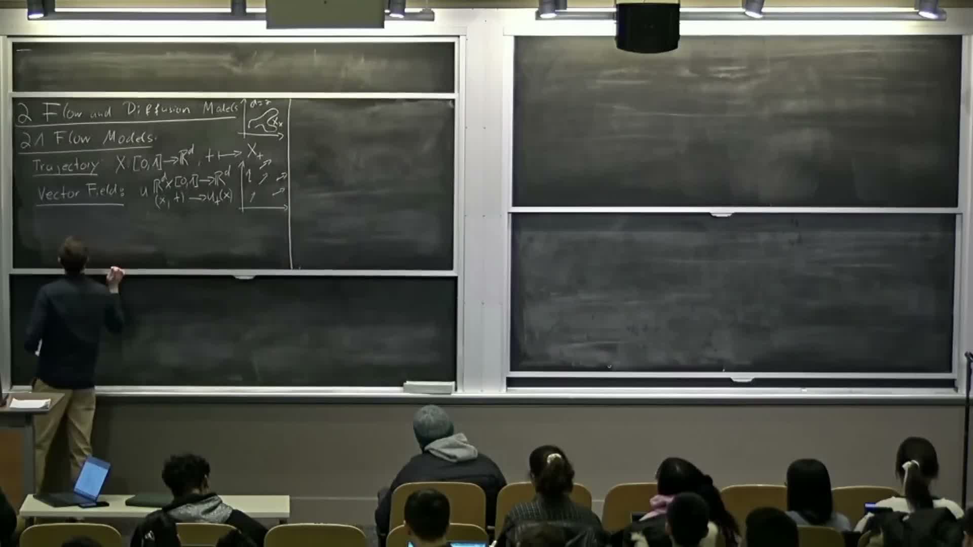
Trajectory: a time-indexed function x(t) mapping a time interval (commonly [0,1]) to R^d — it describes the state of a sample over time.
Vector field: u(t,x) maps each time and spatial location to a velocity vector; it prescribes instantaneous direction and speed.
Ordinary differential equation (ODE): specifies that the time derivative satisfies dx/dt = u(t,x_t) with an initial condition x(0) = x0 — thus trajectories are constrained to follow the instantaneous directions given by the vector field.
Flow map as a collection of ODE solutions and existence/uniqueness conditions
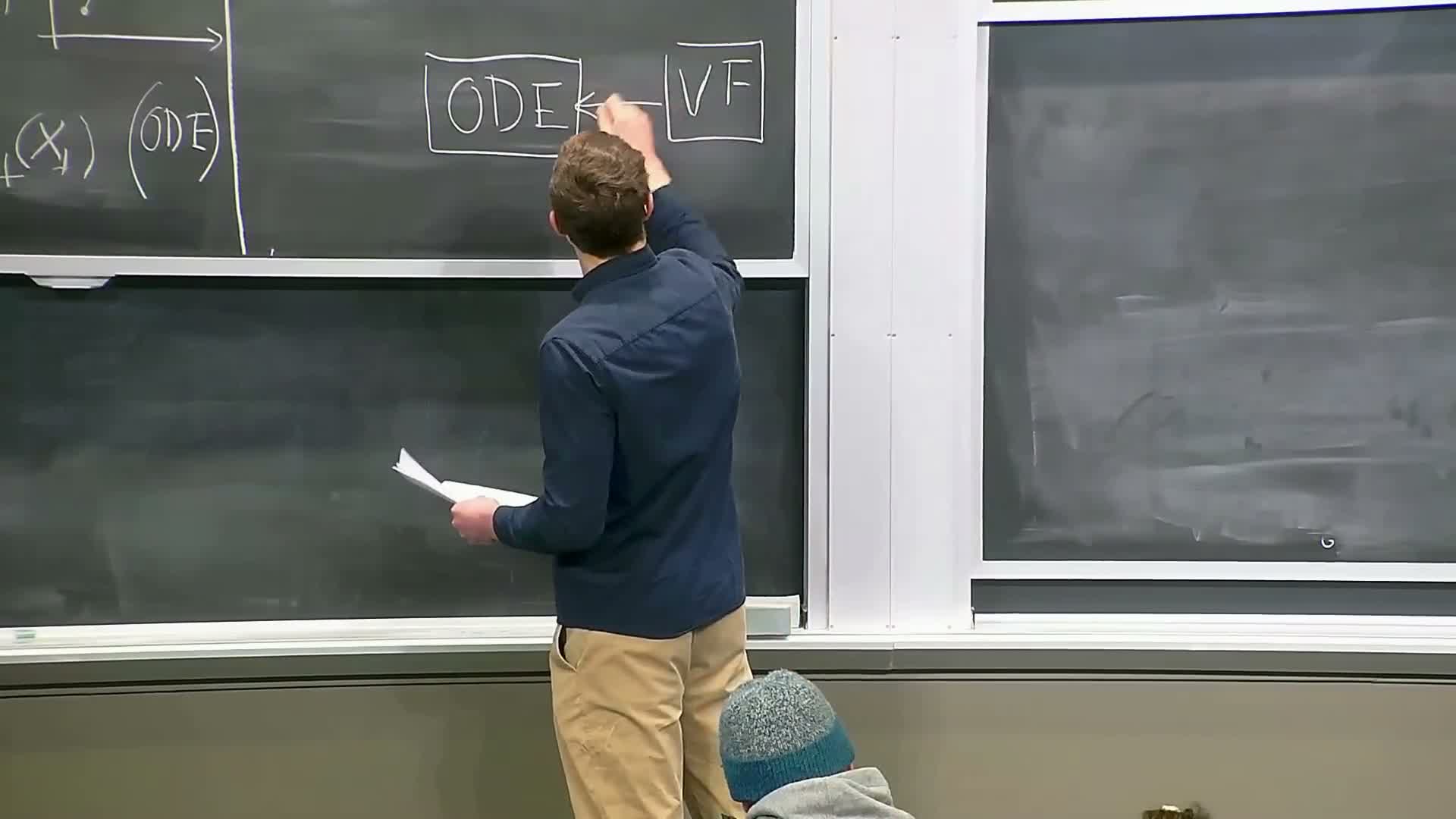
A flow is the family of solutions s_t(x0) obtained by integrating the ODE for all initial conditions x0, producing a time-indexed mapping from initial to evolved states.
Under standard regularity conditions on the vector field (continuous differentiability or Lipschitz continuity with bounded derivatives), existence and uniqueness of solution trajectories — and hence a well-defined flow map — are guaranteed.
Linear vector field example and analytic solution; numerical simulation by Euler method
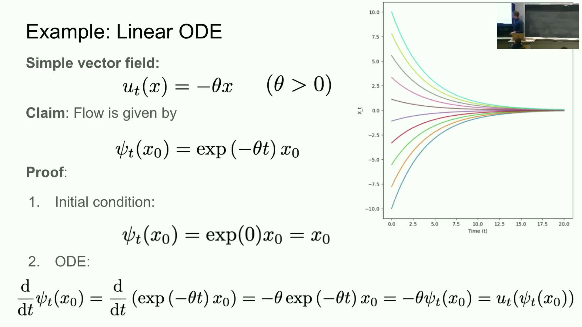
For the linear vector field u(x) = −θ x the ODE solution is s_t(x0) = exp(−θ t) x0, demonstrating exponential contraction.
In general nonlinear cases where closed-form solutions are unavailable, numerical integrators approximate trajectories:
- The explicit Euler method iterates x_{t+h} = x_t + h u(t,x_t).
- The step size h controls numerical accuracy and convergence; smaller h gives better approximations at increased computational cost.
Flow models in machine learning: parameterizing the vector field with neural networks
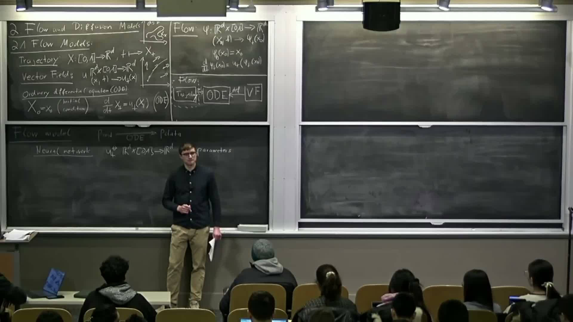
Flow-based generative models parameterize the vector field u_θ(t,x) using a neural network with parameters θ.
Typical workflow:
- Sample an initial state x0 ~ P_init (e.g., Gaussian).
- Integrate the ODE defined by u_θ to obtain the end state x1 via a numerical solver.
- Train (adjust θ) so that the terminal distribution of x1 approximates P_data.
Neural network architecture is chosen per modality (images, video, proteins) to effectively represent the vector field and its time dependence.
Sampling from a flow model and the practical sampling algorithm
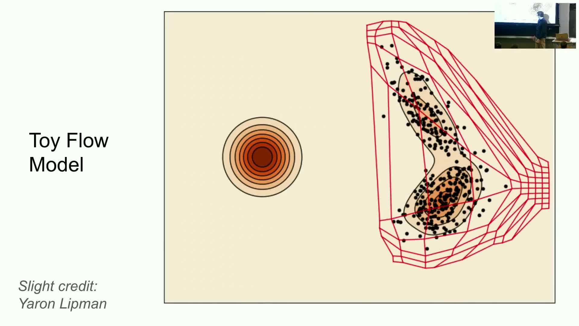
Sampling from a trained flow model is straightforward:
- Draw x0 from the known initial distribution P_init.
- Numerically integrate the ODE using an ODE solver (discretize time, evaluate u_θ at each step).
- Return the terminal state x1 as the generated sample.
In practice this requires repeatedly evaluating the neural-network vector field along the discretized path and updating the state according to the chosen integrator.
Motivation for diffusion models and introduction to stochastic differential equations (SDEs)
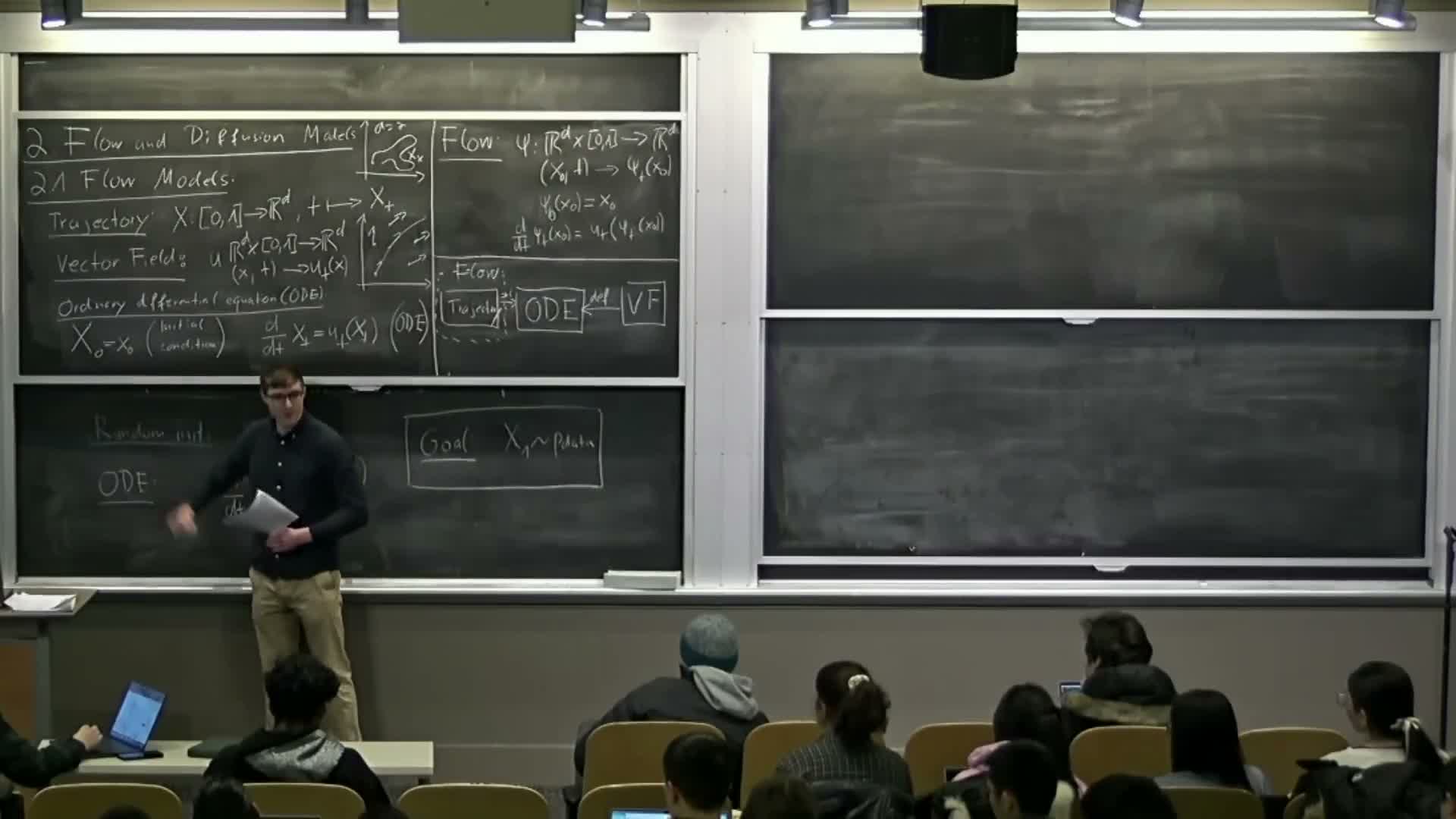
Diffusion models extend deterministic flows by injecting controlled stochasticity during integration.
They model sample evolution as a stochastic process governed by a stochastic differential equation (SDE) that combines:
- a vector field (drift) term u(t,x), and
- a time-dependent diffusion coefficient σ(t) that scales random perturbations.
SDEs allow modeling distributions via both deterministic transport and stochastic exploration within a continuous-time probabilistic framework.
Brownian motion: definition, Gaussian increments and independent increments
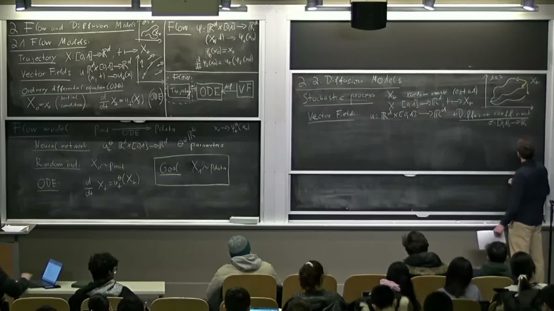
Brownian motion W(t) is the canonical continuous-time stochastic process used for SDEs, characterized by:
-
Continuous sample paths and W(0)=0.
-
Gaussian increments: W(t) − W(s) ~ N(0, (t−s) I) whose variance grows linearly with elapsed time.
-
Independent increments across non-overlapping time intervals.
These properties make Brownian motion the natural continuous analogue of discrete random walks and the standard noise driver in diffusion modeling.
Symbolic SDE notation and discretized increment interpretation
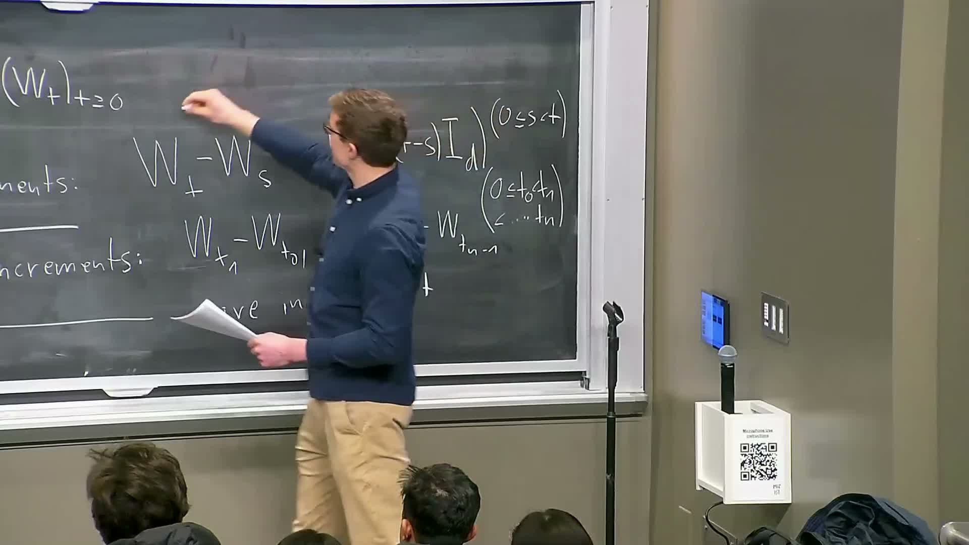
The symbolic SDE notation dx_t = u(t,x_t) dt + σ(t) dW_t is interpreted via its discrete-time increment form:
- For small step h,
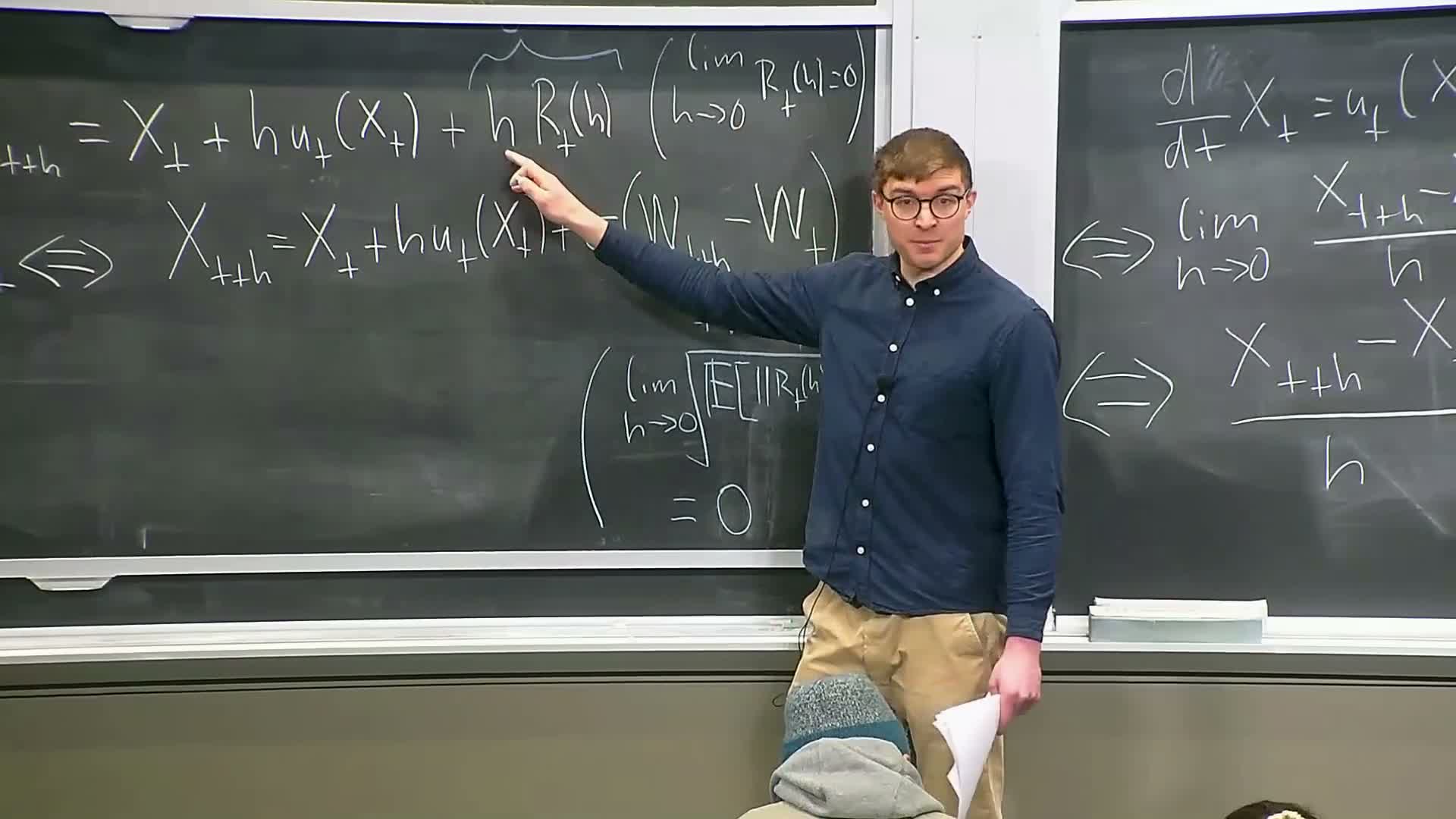
x_{t+h} ≈ x_t + h u(t,x_t) + σ(t) (W_{t+h} − W_t) + r_t(h),
where W_{t+h} − W_t is Gaussian with covariance h I and r_t(h) is a remainder that vanishes as h → 0.
This increment representation replaces classical derivatives (which Brownian paths lack) and forms the basis for simulation and rigorous stochastic integration.
Existence and uniqueness for SDEs and Euler–Maruyama simulation method
Under regularity conditions on the drift u(t,x) (e.g., Lipschitz continuity and bounded derivatives) an SDE admits a unique stochastic process solution.
The standard numerical approximation for simulation is the Euler–Maruyama scheme:
- Iterate x_{t+h} = x_t + h u(t,x_t) + sqrt(h) σ(t) ξ, where ξ ~ N(0,I).
- The scheme samples Gaussian increments scaled by sqrt(h) to match Brownian variance and converges to the SDE solution as the step size decreases.
Ornstein–Uhlenbeck linear SDE example and transition to diffusion model definition
The Ornstein–Uhlenbeck process illustrates a linear SDE with drift −θ x_t and constant diffusion σ, producing mean-reverting dynamics that converge to a Gaussian stationary distribution when σ > 0.
Diffusion generative models adopt the same SDE framework at scale by:
- parameterizing the drift with a neural network, and
- specifying σ(t) (often fixed by design).
The generative objective is that samples initiated from P_init and evolved by the SDE match P_data at the terminal time.
Sampling from diffusion models and practical considerations

Sampling from a diffusion generative model uses the Euler–Maruyama integrator with randomized initial states x0 ~ P_init and iterations:
-
x_{t+h} = x_t + h u_θ(t,x_t) + sqrt(h) σ(t) ξ_t, where ξ_t are independent standard normals.
Practical considerations:
- Choose σ(t) schedules to trade off exploration and numerical stability.
- Implement conditioned generation by feeding conditioning variables into u_θ.
- Focus on final-time samples x1 as the generated outputs.
Course logistics, evaluation and resources
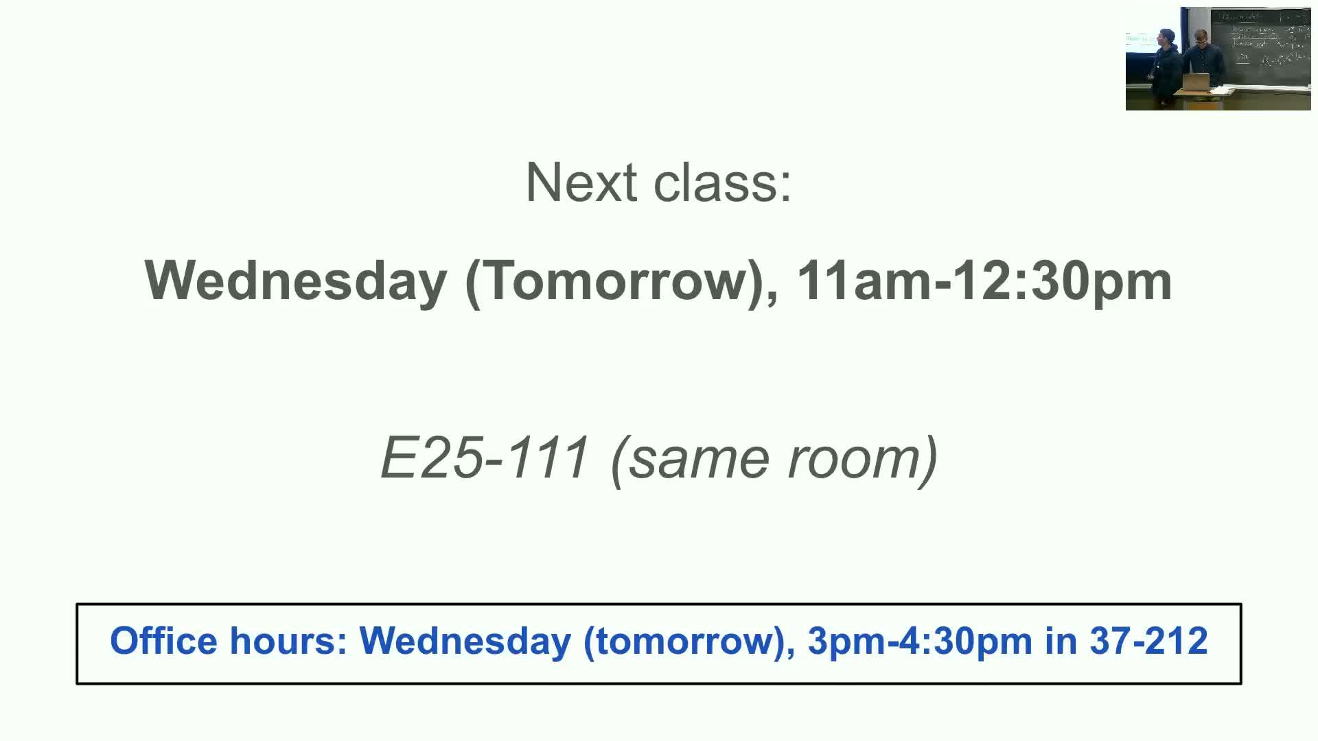
Course logistics and assessment:
- Passing requires attendance or recorded lecture review plus lab completion.
- Points are allocated across lectures and labs, and labs are submitted via provided GitHub notebooks.
- Primary study resources are the course lecture notes (self-contained) and office hours for lab help.
- The first lab implements basic sampling from flows and SDEs and is provided with specified deadlines and grading procedures.
Enjoy Reading This Article?
Here are some more articles you might like to read next: